Matching Structural Densities from Different Biophysical Origins with Gain and Bias

Abstract

The registration of volumetric structures in real space involves geometric and density transformations that align a target map and a probe map in the best way possible. Many computational docking strategies exist for finding the geometric transformations that superimpose maps, but the problem of finding an optimal density transformation, for the purposes of difference calculations or segmentation, has received little attention in the literature. We report results based on simulated and experimental electron microscopy maps, showing that a single scale factor (gain) may be insufficient when it comes to minimizing the density discrepancy between an aligned target and probe. We propose an affine transformation, with gain and bias, that is parameterized by known surface isovalues and by an interactive centering of the “cancellation peak” in the surface thresholded difference map histogram. The proposed approach minimizes discrepancies across a wide range of interior densities. Owing to having only two parameters, it avoids overfitting and requires only minimal knowledge of the probe and target maps. The linear transformation also preserves phases and relative amplitudes in Fourier space. The histogram matching strategy was implemented in the newly revised volhist tool of the Situs package, version 2.6.

Introduction

The registration of 3D maps in structural biology relies on applying suitable operations to a probe and a target map such that they match as closely as possible. This task is most often dealt with in the context of some geometric transformation, such as in rigid-body or flexible docking (Mendelson and Morris, 1997; Wriggers and Chacón, 2001a; Siebert and Navaza, 2009). Here, we focus on density difference calculations or segmentation, where the registration task requires an additional density transformation between the two maps. We present a real example from our work, where the traditional approach of scaling the probe map by a single gain factor failed to minimize density discrepancies: this example involves matching between a 3D cryo-electron microscopy (cryo-EM) reconstruction of the frozen-hydrated tarantula thick filament and a simulated map from a fitted atomic model of heavy meromyosin (HMM) that contains two myosin S1 heads plus the S2 segment.

Figure 1 shows the biological system of interest and the modeling work flow that involves difference calculations and segmentation. The map editing steps were employed in the recent flexible refinement of the HMM atomic model against the cryo-EM data (Alamo et al., 2008). The goal was to obtain an isolated HMM map that retained the shape of the interactinghead motif in the cryo-EM map (Fig. 1A), but without extra densities from (helical-symmetric) neighboring myosin heads or sub-filament backbone. After isolating and subtracting the foreign densities from the cryo-EM map, the final result (Fig. 1D) retains all of the cryo-EM features, except that new molecular boundaries were introduced (when necessary) using the matched atomic model of HMM as a mask. The final map in (Fig. 1D) has no extra densities compared to the atomic model in (Fig. 1B); this is an important prerequisite for subsequent flexible fitting (Alamo et al., 2008).

Figure 1.

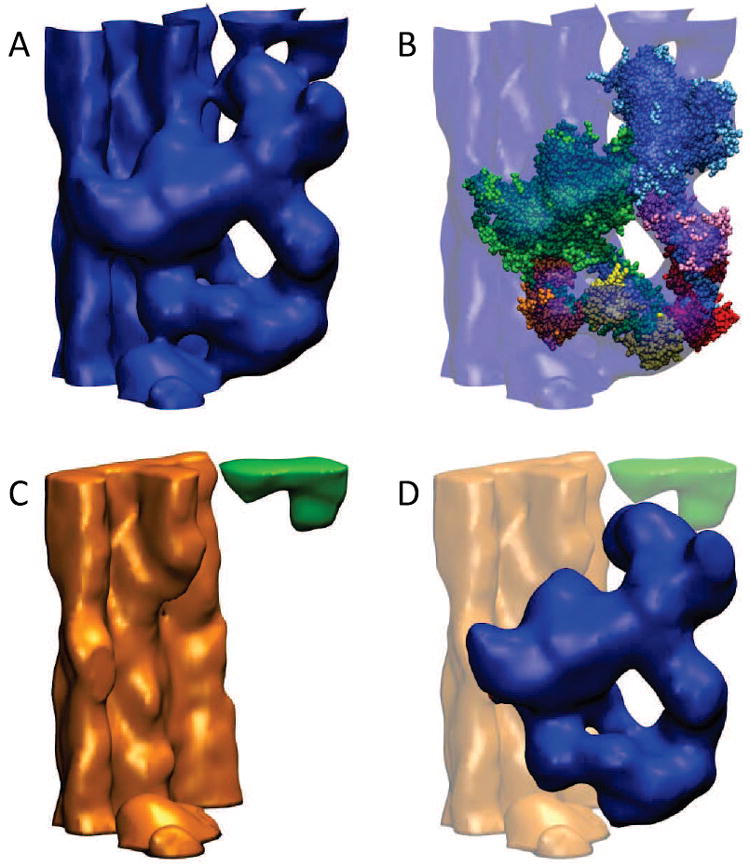
The role of volumetric density matching and subtraction in multi-scale modeling. (A) Helical 3D reconstruction of the frozen-hydrated tarantula thick filament filtered to 20 Å resolution (Alamo et al., 2008), cropped here with voledit (Wriggers, 2010) to a single interacting-head motif that corresponds to two myosin S1 heads plus the S2 coiled coil and the sub-filament region behind them. (B) HMM atomic model fitted to the interacting-head motif. The model was built from a chicken smooth muscle HMM model (Liu et al., 2003), refined from Protein Data Bank entry 1I84 and kindly provided by Kenneth Taylor. The HHM model without the S2 was fitted to the cryo-EM map with colores (Chacón and Wriggers, 2002) and the S2 of the model was replaced by two unconnected segments of a double alpha-helix that allowed us to carry out a hand fitting of these segments to follow the S2 volume densities in the cryo-EM map. (C) Two isolated volumes, thick filament bundle with neighboring free head (orange) and neighboring blocked head (green), which were obtained by segmentation with voledit after subtraction of the (simulated) density of the fitted HMM atomic model with voldiff. The simulated density (not shown) was created by Gaussian convolution at resolution 20 Å, using pdb2vol. (D) The isolated HMM cryo-EM density (blue) after subtraction of the two segments of (C) from the full map shown in (A). For clarity, we have omitted the segmentation and modeling of the myosin S1 regulatory light chain regions described in Alamo et al. (2008). Figures 1 and 2 were created with the Situs package (Wriggers, 2010) and with the molecular graphics program VMD (Humphrey et al., 1996).

Real-space modeling is a “WYSIWYG” (what you see is what you get) approach. Leaving aside geometric transformations, we apply elementary “volume algebra” operations to voxels that are small in number, intuitive, and can be easily learned and used. Figure 1 provides examples of such volume algebra operations and operands supported by Situs (Wriggers, 2010) that allow the expression of volume-to-volume and structure-to-volume transformations in biophysical modeling applications:

• cropping, where densities outside the region of interest are set to zero or cut from the map (Fig. 1A);

• segmentation, where a contiguous volume above an isovalue threshold is extracted from the background with the floodfill algorithm (Fig. 1C,D);

• resolution-lowering (also called low-pass filtering, using the spectral analogy), where a simulated map is created from higher resolution data (not shown, but the technique is common (Belnap et al., 1999) and we support it in the form of convolution with Gaussian and other kernels);

• thresholding, where densities below an isovalue cutoff are set to zero (Fig. 1C,D);

• subtraction, where the discrepancy of densities is computed (Fig. 1C,D) to simulate the molecular boundaries between individual segments (Volkmann et al., 2000); and finally

• density matching, the focus of this paper.

Figure 2 demonstrates the density matching problem we encountered when subtracting the simulated EM map from the cryo-EM data in Fig. 1C. The proper cancellation of densities during subtraction is critical for defining the molecular boundaries between individual segments; this affects the stereochemical quality of downstream flexibly fitted structures as in Alamo et al. (2008). The traditional approach is to rescale the densities of one of the maps such that the isosurfaces of the known molecular surfaces match (one needs to know only the approximate isovalue of one map; the matching isovalue of the other map can then be estimated interactively with a molecular graphics program, see below). Figure 2A shows that this approach is insufficient to remove all of the interior densities of the interacting-head motif from the discrepancy map. One can attempt to “overscale” the subtracted simulated HMM map by a factor of 1.5 or 2 (Fig. 2B,C) to remove the interior densities; however, this would introduce strong negative densities into the discrepancy map and erode the molecular boundaries of the sub-filament and neighbor densities one wants to isolate in the work flow (Fig. 1C). Clearly, the cryo-EM map exhibits much higher densities in its interior compared to those of the surface-matched simulated HMM map, and any scaling factor produces suboptimal cancellation of interior densities.

Figure 2.

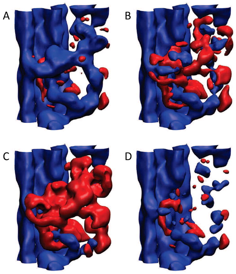
Effect of various scaling factors (A-C) and optimal affine transformation (D) on the difference map between the original reconstruction (Fig. 1A) and the (simulated) map obtained from the HMM atomic model (Fig. 1B). The isocontours correspond to the surface density (blue) of the original map and its negative (red). (A) Simulated HMM map scaled with volhist (Wriggers, 2010) to match surface isovalues before subtraction with voldiff. (B) As in (A), but additional scaling factor of 1.5 applied to the surface-matched HMM map before its subtraction. (C) As in (A), but additional scaling factor of 2.0 applied to the surface-matched HMM map before its subtraction. (D) Optimal affine transformation (see text): The original map (Fig. 1A) was density matched to the simulated HMM map before subtraction of the simulated map.

The solution we propose in this paper is to use an affine transformation, including gain and bias, for the density matching. The linear transformation preserves phases and relative amplitudes in Fourier space, which is important for many biophysical data sets that are derived wholly or in part with Fourier techniques (for example, if one wishes to calculate theoretical diffraction patterns from any part of a map subject to “volume algebra”). The bias value adds a constant to the zero-frequency Fourier component, which is often poorly determined: In EM image processing, the underlying 2D images are often “floated” prior to 3D reconstruction to prevent edge effects (DeRosier and Moore, 1970), and the background densities within the same micrograph field can vary by a significant margin as the result of uneven ice thickness and other factors (Zhang et al., 2008). Therefore, it seems prudent to use a transformation that optimizes only the weakly or unconstrained parameters (such as bias and global gain factor), while retaining critical structural information such as relative amplitude and phases of Fourier components. Figure 2D demonstrates that a satisfying cancellation of densities can be achieved by an affine transformation. Only a few features remain in the final discrepancy map: These biologically relevant differences are caused by missing regulatory light chain regions and density shifts from conformational changes (Alamo et al., 2008).

The remainder of the paper is organized as follows. After introducing the mathematical notation in Methods, we describe the parameterization of the transformation model and justify our choice of interactive optimization by means of a surface thresholded discrepancy map histogram. Next, we describe the semi-automated implementation of our approach in the Situs package. We revisit the HMM matching example in Results and Discussion, and demonstrate the method’s robustness. In Conclusions we comment on the usability, advantages, and limitations of this method and on future work.

Methods

Let ρ₁ > 0 denote the target map and ρ₂ > 0 the probe map whose density should be matched to ρ₁. In most applications, one would use the more reliable map as the target (for example, a simulated map derived from an atomic structure can be a suitable target because it is free from any noise or systematic artifacts introduced by a particular biophysical structure determination technique). Let s₁ > 0 and s₂ > 0 be the suitably chosen surface isovalues of ρ₁ and ρ₂, respectively. We assume an increasing affine density transformation model with gain σ and bias β that matches the surface isovalues:

$${\stackrel{\sim }{\rho }}_2(\beta )=\sigma (\beta )\cdot {\rho }_2+\beta ,$$ (1)

$$\sigma (\beta )=\frac{s_1-\beta }{s_2},$$ (2)

where β < s₁ is a user-selectable parameter that can be negative, and ρ̃₂ denotes the probe density matched to ρ₁ via the affine transformation.

In the following, we are concerned only with the interior densities ρ₁ ≥ s₁ and ρ̃₂ ≥ s₁. Let ⋯∣_c denote the thresholding at isovalue c, i.e., all densities below c are set to zero. We define the surface-thresholded discrepancy map as

$${\mathrm{\Delta }}_{12}(\beta )={\rho }_1{\mid }_{s_1}-{\stackrel{\sim }{\rho }}_2{\mid }_{s_1}(\beta ).$$ (3)

Figure 3A illustrates the features of the discrepancy map. The densities will (partially) cancel in the map overlap region, but there will be also some non-overlapping densities outside of the overlap region. The thresholding at s₁ in Eqn. 3 ensures that unreliable “exterior” densities from either map do not enter Δ₁₂: In cryo-EM reconstructions, low exterior densities are typically caused by the ice background, noise, and/or numerical ringing from Fourier techniques in the reconstruction process (Frank, 1996).

Figure 3.

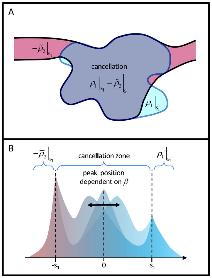
Interactive optimization of the affine transformation (schematic illustration). (A) Density cancellation between overlapping thresholded densities ρ₁∣_s1 and ρ̃₂∣_s1. (B) Adjustment of the free bias parameter β centers the peak in the “cancellation zone” of the trimodal histogram of Δ₁₂ ≠ 0. The gain value depends implicitly on the selected bias (see Eqn. 2).

The optimization of Eqn. 1 as a function of β could be performed by systematically minimizing the discrepancies Δ₁₂. However, when inspecting the histogram of Δ₁₂ (shown schematically in Fig. 3B, actual results for the HMM example are given in Fig. 4), we found that deciding which values to minimize would be non-trivial and somewhat arbitrary: The Δ₁₂ distribution has significant outliers resulting from non-overlapping densities, and any cancellation of densities is incomplete. Figure 3B illustrates that the distribution of Δ₁₂ ≠ 0 is trimodal, exhibiting sharp peaks at ±s₁ (due to thresholding and non-overlapping densities) and a broader peak in the central “cancellation zone” [−s1,⋯, s1]. We found that the position and shape of the cancellation peak depends sensitively on β. Although the target and probe densities do not cancel perfectly, it is reasonable to expect this cancellation peak to be centered at zero for the optimal affine transformation (it would be a delta function in the ideal case of perfect cancellation).

Figure 4.

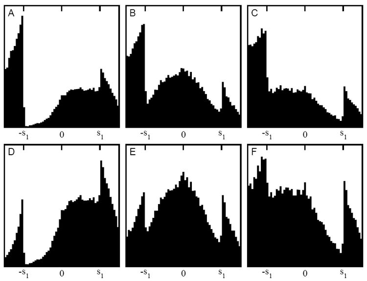
Interactive optimization of the affine transformation (observed data). Shown here are central sections of the histogram of Δ₁₂ ≠ 0 for the simulated (HMM model-derived) target map ρ₁, and either the full (Fig. 1A) or the isolated (Fig. 1D) probe map ρ₂ in (A-C) or (D-F), respectively. In the left panels (A,D), β is too high (and σ is too low); in the middle panels (B,E), the transformation is optimal; and in the right panels (C,F), β is too low (and σ is too high). The result (B) was used for the difference map shown in Fig. 2D. The specific numerical values of user-defined parameters were: s₁ = 20.0, s₂ = 30.0, β = 14.0, 8.0, and 2.0 (from left to right), and σ = 0.2, 0.4, and 0.6 (from left to right).

We have added an interactive optimization approach to the existing volhist tool of the Situs package. When prompted with two input maps, the program asks for input of the s₁ and s₂ values. The histogram of Δ₁₂(β) ≠ 0 is then plotted for user-selected values β < s₁ until the user is satisfied with the centering of the cancellation peak. Finally, the program writes the transformed map ρ̃₂∣₀ to an output file.

Results and Discussion

The proposed affine transformation was applied successfully to the biological HMM example (Figs. 2D and 4). In Figure 4, we demonstrate the effect of the β parameter on the shape of the cancellation peak. The peak shape and position are sensitive to β, and the visual inspection of the histogram is deemed an appropriate criterion for finding the optimal transformation. The shape and position of the peak remained robust when comparing two different probe maps that both contained the interacting-head motif (Fig. 4). This robustness is important, because the trimodal histogram of Δ₁₂ appears most symmetric when all densities are accounted for and the probe and target maps are similar in shape (Fig. 4E). However, in a realistic work flow, one would often compare a subunit to a larger map with significant extraneous unmatched density (Fig. 1B), yielding asymmetric outer peaks in the histogram, as shown in Fig. 4B. This asymmetry of the outer peaks does not influence the cancellation peak or the optimum β value. The HMM system was chosen for the demonstration because the method originated in our work on tarantula thick filament and the matching required a significant bias. We have tested the approach on various other EM systems and the trimodal appearance of Δ₁₂ remained robust.

An important initial step in parameterization is the estimation of the surface isovalues s₁ and s₂. There is no rigorous way to calculate the surface of an EM map. In most cases, a microscopist provides an empirical isocontour value that encloses about 120-150% of the atomic resolution volume. Resolution lowering erodes convex (and fills up concave) features of the surface. Therefore, to give a subjectively similar-looking surface and to prevent convex features from protruding from the surface, the enclosed EM volume is somewhat higher than the atomic volume. One could choose to use some criterion based on edge detection, such as the Laplacian (Chacón and Wriggers, 2002), but such a surface would cover a range of density levels, i.e., this approach might be similarly “ad hoc” as the volume criterion. Interestingly, the EMDB database (Tagari et al., 2002) has no consistent standard for the surface isocontour. The majority of “recommended contour levels” found in EMDB headers were determined empirically to create the meshes used in their EMviewer software. Only newer maps deposited since 2009 have author-recommended contour levels. We agree with the new EMDB standard that the depositing authors should know best. Fortunately, the exact knowledge of absolute surface isocontours is not so critical for our parameterization. Even if the surface level s₂ is known only approximately, one can achieve a suitably precise surface match through the interactive adjustment of the isovalue s₁ in a Situs compatible molecular graphics package such as VMD (Humphrey et al., 1996), Chimera (Pettersen et al., 2004), or Sculptor (see article by Birmanns et al. in this issue).

We have decided to implement only a limited thresholding in the output map ρ̃₂∣₀ to remove any non-physical negative densities introduced by β < 0. For positive biases, no thresholding is applied to the transformed map. This means that the map background is shifted from zero to a level β < s₁. We found that this shift in background was inconsequential for our work as long as maps and difference maps were rendered at the s₁ isolevel or above (Fig. 2D). If needed, a user could threshold the output map at or below the s₁ level in a post-processing segmentation step (using voledit), to bring any positive background to zero.

Conclusions

We propose an affine transformation, with gain and bias, that is parameterized by known surface isovalues and by an interactive centering of the cancellation peak in the surface thresholded difference map histogram. To our knowledge, the simple yet effective transformation has not been applied before in the context of difference mapping and segmentation (Fig. 1), but the density matching problem is known in the EM community. For example, Roseman (2000) justified his masked cross-correlation criterion for finding an optimal geometric match in terms of its ability to automatically take background density variations into account. Here, we were less concerned with docking, but rather were focused on difference mapping and resolution lowering. This required us to introduce an explicit bias to deal with “solvent surrounding the specimen in order to match the search object and the EM map because solvent is not included in the density-search object calculated from the atomic coordinates” (Roseman, 2000). Our affine approach is also expected to be useful for matching low-resolution maps derived from smallangle X-ray bead models (Wriggers and Chacón, 2001b), because these maps exhibit a flatter interior density profile compared to simulated maps.

An affine transformation is performed implicitly in many docking applications that maximize the Pearson correlation coefficient (Wriggers and Chacón, 2001a). There are, however, some key differences between our proposed approach and the shift and scaling afforded by the correlation coefficient. The use of least-squares fitting of the maps (implicitly performed by maximizing the correlation) is not suitable for difference mapping and segmentation (the application purpose of this paper) because the least-squares approach is sensitive to density outliers which typically occur in such difference maps (Fig. 4). As described in Methods, a minimization of the squared discrepancies Δ₁₂ would take into account mainly the outliers, whereas one would really wish to perform a centering of the peak in the (bias-dependent) cancellation zone. Also, a key step in our approach is the thresholding by the surface value s₁ which is independent of the correlation coefficient. We verified that it is not possible to match densities without thresholding by s₁: The difference map histograms would become unusable since exterior densities that are not removed by thresholding would spoil the discrepancies in the cancellation zone.

We note also that photometric (as opposed to geometric) density matching is well known in the related field of 2D image registration: A simple photometric transformation applied to the pixel intensities, for example gain and bias, can account well for differences in global lighting of images (Bartoli, 2006). We have also experimented with more sophisticated nonlinear histogram matching techniques used in the image processing community (Yu and Bajaj, 2004). Our work showed that there is a risk of overfitting density levels at the high and low ends of the distribution (Cooper and Wriggers, unpublished). Furthermore, the nonlinear transformation would not preserve the structure factors (Fourier spectrum). As a result, we have abandoned this idea in favor of the current linear approach.

In the present implementation the centering of the cancellation peak is performed interactively. An automation of this step is not critical for the work flow shown in Figure 1 since it is performed only once. If an automation is desired in future work it could be implemented using e.g. a Gaussian based density estimator for the Δ₁₂ peak in the cancellation zone. Such an automation would also open up the possibility of calculating the proposed affine transformation on the fly during a geometric docking search. The beneficial effects of density masking (Roseman, 2000) suggest that our position-dependent thresholding and linear transformation could improve the docking precision. For such a hypothetical future application in docking one would also need to automate the estimation of the s₁ (masking) threshold, if s₁ depends on the parts of the target map a probe molecule overlaps with.

In summary, we expect the proposed affine transformation to be generally useful in applications of difference mapping and segmentation, especially if 3D maps are derived from diverse biophysical origins, such as EM, tomography, low-resolution crystallography, small-angle (X-ray or neutron) scattering, and simulated maps derived from atomic structures. The volhist tool can be freely downloaded as part of the Situs package at URL http://situs.biomachina.org.

References

- Alamo L, Wriggers W, Pinto A, Bártoli F, Salazar L, Zhao F-Q, Craig R, Padrón R. Three-dimensional reconstruction of tarantula myosin filaments suggests how phosphorylation may regulate myosin activity. J Mol Biol. 2008;384:780–797. doi: 10.1016/j.jmb.2008.10.013. [DOI] [PMC free article] [PubMed] [Google Scholar]
- Bartoli A. Topics in Automatic 3D Modeling and Processing Workshop. Verona, Italy: 2006. Direct image registration with gain and bias. [Google Scholar]
- Belnap DM, Kumar A, Folk JT, Smith TJ, Baker TS. Low-resolution density maps from atomic models: How stepping “back” can be a step “forward”. J Struct Biol. 1999;125:166–175. doi: 10.1006/jsbi.1999.4093. [DOI] [PubMed] [Google Scholar]
- Chacón P, Wriggers W. Multi-resolution contour-based fitting of macromolecular structures. J Mol Biol. 2002;317:375–384. doi: 10.1006/jmbi.2002.5438. [DOI] [PubMed] [Google Scholar]
- DeRosier DJ, Moore PB. Reconstruction of three-dimensional images from electron micrographs of structure with helical symmetry. J Mol Biol. 1970;52:355–369. doi: 10.1016/0022-2836(70)90036-7. [DOI] [PubMed] [Google Scholar]
- Frank J. Three-Dimensional Electron Microscopy of Macromolecular Assemblies. Academic Press; San Diego: 1996. [Google Scholar]
- Humphrey WF, Dalke A, Schulten K. VMD – Visual Molecular Dynamics. J Mol Graphics. 1996;14:33–38. doi: 10.1016/0263-7855(96)00018-5. [DOI] [PubMed] [Google Scholar]
- Liu J, Wendt T, Taylor D, Taylor K. Refined model of the 10S conformation of smooth muscle myosin by cryo-electron microscopy 3D image reconstruction. J Mol Biol. 2003;329:963–972. doi: 10.1016/s0022-2836(03)00516-3. [DOI] [PubMed] [Google Scholar]
- Mendelson R, Morris EP. The structure of acto-myosin subfragment 1 complex: Results of searches using data from electron microscopy and x-ray crystallography. Proc Natl Acad Sci USA. 1997;94:8533–8538. doi: 10.1073/pnas.94.16.8533. [DOI] [PMC free article] [PubMed] [Google Scholar]
- Pettersen EF, Goddard TD, Huang CC, Couch GS, Greenblatt DM, Meng EC, Ferrin TE. UCSF Chimera - A visualization system for exploratory research and analysis. J Comp Chem. 2004;25:1605–1612. doi: 10.1002/jcc.20084. [DOI] [PubMed] [Google Scholar]
- Roseman AM. Docking structures of domains into maps from cryo-electron microscopy using local correlation. Acta Cryst D. 2000;56:1332–1340. doi: 10.1107/s0907444900010908. [DOI] [PubMed] [Google Scholar]
- Siebert X, Navaza J. UROX 2.0: an interactive tool for fitting atomic models into electron-microscopy reconstructions. Acta Cryst D. 2009;65:651–658. doi: 10.1107/S0907444909008671. [DOI] [PMC free article] [PubMed] [Google Scholar]
- Tagari M, Newman R, Chagoyen M, Carazo JM, Henrick K. New electron microscopy database and deposition system. Trends Biochem Sci. 2002;27:589. doi: 10.1016/s0968-0004(02)02176-x. [DOI] [PubMed] [Google Scholar]
- Volkmann N, Hanein D, Ouyang G, Trybus KM, DeRosier DJ, Lowey S. Evidence for cleft closure in actomyosin upon ADP release. Nature Struct Biol. 2000;7:1147–1155. doi: 10.1038/82008. [DOI] [PubMed] [Google Scholar]
- Wriggers W. Using Situs for the integration of multi-resolution structures. Biophysical Reviews. 2010;2:21–27. doi: 10.1007/s12551-009-0026-3. [DOI] [PMC free article] [PubMed] [Google Scholar]
- Wriggers W, Chacón P. Modeling tricks and fitting techniques for multi-resolution structures. Structure. 2001a;9:779–788. doi: 10.1016/s0969-2126(01)00648-7. [DOI] [PubMed] [Google Scholar]
- Wriggers W, Chacón P. Using Situs for the registration of protein structures with low-resolution bead models from X-ray solution scattering. J Appl Cryst. 2001b;34:773–776. [Google Scholar]
- Yu Z, Bajaj C. A fast and adaptive method for image contrast enhancement. Int Conf on Image Processing (ICIP) 2004 Oct;:1001–1004. [Google Scholar]
- Zhang W, Kimmel M, Spahn CMT, Penczek PA. Heterogeneity of large macromolecular complexes revealed by 3D cryo-EM variance analysis. Structure. 2008;16:1770–1776. doi: 10.1016/j.str.2008.10.011. [DOI] [PMC free article] [PubMed] [Google Scholar]