Stability of resting fMRI interregional correlations analyzed in subject-native space: a one-year longitudinal study in healthy adults and premanifest Huntington’s disease

Abstract

The pattern of interregional functional MRI correlations at rest is being actively considered as a potential noninvasive biomarker in multiple diseases. Before such methods can be used in clinical studies it is important to establish their usefulness in three ways. First, the long-term stability of resting correlation patterns should be characterized, but there have been very few such studies. Second, analysis of resting correlations should account for the unique neuroanatomy of each subject by taking measurements in native space and avoiding transformation of functional data to a standard volume space (e.g., Talairach-Tournox or Montreal Neurological Institute atlases). Transformation to a standard volume space has been shown to variably influence the measurement of functional correlations, and this is a particular concern in diseases which may cause structural changes in the brain. Third, comparisons within the patient population of interest and comparisons between patients and age-matched controls, should demonstrate sensitivity to any disease-related disruption of resting functional correlations. Here we examine the test-retest stability of resting fMRI correlations over a period of one year in a group of healthy adults and in a group of cognitively intact individuals who are gene-positive for Huntington’s disease. A recently-developed method is used to measure functional correlations in the native space of individual subjects. The utility of resting functional correlations as a biomarker in premanifest Huntington’s disease is also investigated. Results in control and premanifest Huntington’s populations were both highly consistent at the group level over one year. We thus show that when resting fMRI analysis is performed in native space (to reduce confounds in registration between subjects and groups) it has good long-term stability at the group level. Individual-subject level results were less consistent between visit 1 and visit 2, suggesting further work is required before resting fMRI correlations can be useful diagnostically for individual patients. No significant effect of premanifest Huntington’s disease on prespecified interregional fMRI correlations was observed relative to the control group using either baseline or longitudinal measures. Within the premanifest Huntington’s group, though, there was evidence that decreased striatal functional correlations might be associated with disease severity, as gauged by estimated years to symptom onset or by striatal volume.

1 Introduction

There is currently great interest in measuring interregional correlations of the resting blood oxygenation level dependent (BOLD) fMRI signal (Biswal et al., 1995) as a biomarker in disease. This approach could have advantages over structural MRI as it might reveal changes in physiological function before widespread and substantial cell loss occurs (Bohanna et al., 2008). Resting fMRI has a strong clinical appeal because it affords the ability to study multiple networks of the entire brain at once and without confounding effects of cognitive ability to perform a given behavioral task (Auer, 2008; Fox and Raichle, 2007; Greicius, 2008; van den Heuvel and Hulshoff Pol, 2010; Rogers et al., 2007; Petrella 2011). Already, variations in resting functional correlations (often termed “functional connectivity”) have been reported in a wide range of neurological and psychiatric disorders, including Alzheimer’s disease (Greicius et al., 2004; Sorg et al., 2009), mild cognitive impairment (Bai et al., 2009; Pihlajamäki et al., 2009; Sorg et al., 2007), amyotrophic lateral sclerosis (Mohammadi et al., 2011b), schizophrenia (Jafri et al., 2008; Repovs et al., 2011), depression (Greicius, 2008), writer’s cramp (Mohammadi et al., 2011a), and Parkinson’s disease (Helmich et al., 2010; Wu et al., 2009). In the case of amyloid-associated pathology, there is evidence that resting functional correlations may be sensitive to neurological changes prior to onset of clinical symptoms (Hedden et al., 2009; Sheline et al., 2010). Taken together, these many reports motivate resting fMRI as a tool for investigating the disease process across time (i.e. in longitudinal biomarker studies) with the eventual aim of evaluating neuroprotection or treatment.

It is important, however, to first evaluate the test-retest stability of resting fMRI. Stability may be a particular concern in resting fMRI because whereas task-based studies attempt to tightly control brain behavior, resting fMRI uses an unconstrained paradigm that allows the potential for markedly different states of mental activity from one scan session to the next. Existing studies of stability in resting fMRI have used data transformed to a standard volume (Chen et al., 2008; Damoiseaux et al., 2006; Meindl et al., 2010; Shehzad et al., 2009; Thomason et al., 2011; Van Dijk et al., 2009; Zuo et al., 2010), and to our knowledge, only one data set has been examined with longitudinal measurements in adults (mean age 20.5 years) for a period longer than 16 days (5–16 months) (Shehzad et al., 2009). Thus, further investigation of the long-term stability of resting functional correlations is needed.

For resting fMRI to be a useful biomarker in neurological disease it may also be necessary to use an analysis method that takes into account the fact that patient or gene-positive groups may already have changes in gray and white matter for example, to regions adjacent to cerebrospinal fluid, such as the periventricular basal ganglia regions. When such changes occur, it is possible that resting correlations can be mistakenly measured from voxels in white matter or cerebrospinal fluid (Krishnan et al., 2006). We recently showed that transforming functional data to a standard volume (e.g., Talairach or MNI152) can introduce large, widespread effects on resting fMRI correlations due to imperfect registration of native anatomy to the volume atlas (Seibert and Brewer, 2011). This was true even in young, healthy subjects, but is a particular concern in disease. We proposed an alternative method that addresses these issues by analyzing resting BOLD correlations on models of the native cortical surface created for each subject’s brain (Seibert and Brewer, 2011). Here we again apply this native-space method.

Finally, the utility of resting fMRI to biomarker development also requires establishing that longitudinal inter-regional correlations can indeed detect differences between a disease group and a healthy one. Huntington’s disease (HD) is a genetic neurodegenerative disorder that causes deficits in both motor and cognitive function. Though HD affects a number of brain regions, including cerebral cortex, the most prominent neuropathologic changes occur in the striatum, made up of the caudate and putamen (Eidelberg and Surmeier, 2011; Rosas et al., 2008). Strikingly, atrophy in the caudate and putamen has been identified using neuroimaging more than a decade prior to the estimated onset of manifest symptoms, i.e. during the premanifest stage of HD (pre-HD) (Aylward et al., 1996, 2004, 2011; Paulsen et al., 2010; Stoffers et al., 2010; Tabrizi et al., 2009). In this study, we compare gene-positive premanifest HD participants with a group of healthy controls matched for age and IQ.

Diagnosis of Huntington’s disease is aided by the presence of genetic markers, and these genetic markers permit identification of high-risk individuals prior to onset of clinical symptoms. An imaging biomarker is highly desirable in premanifest Huntington’s disease (pre-HD) to track progression, inform prognosis, and measure the effects of potential therapies. We have previously shown that MRI can detect structural changes (atrophy) over one year in pre-HD (Majid et al., 2011). A functional MRI technique might complement structural MRI and suggest physiological relevance of structural changes; additionally, functional imaging may have the potential to detect acute effects of therapies before major structural pathology occurs (Rosas et al., 2004). Differences between pre-HD and age-matched control populations have already been demonstrated using task-based fMRI (Klöppel et al., 2009; Paulsen et al., 2004; Reading et al., 2004; Wolf et al., 2008; Zimbelman et al., 2007), but disease-related changes in functional activation have yet to be identified longitudinally in pre-HD, and resting fMRI correlations have not been evaluated in pre-HD.

Thus, the present study had two main objectives. First, we aimed to investigate the long-term stability (over one year) of resting fMRI correlations in 22 healthy adults and also 34 adults with pre-HD. Second, we aimed to ascertain whether a detectable difference exists in the resting interregional functional correlations between pre-HD subjects and age-matched controls (cross-sectionally and longitudinally). Importantly, to avoid artifactual effects from transformation to a standard volume, functional correlations in this study are calculated on each subject’s native cortical surface and within native-space subcortical structures.

2 Methods

2.1 Subjects

Thirty-seven pre-HD (≥ 38 CAG repeats) and 22 healthy age-matched control participants underwent resting state scans at two visits, with a one-year interval between visits. Consent was provided in accordance with an Institutional Review Board at the University of California, San Diego. A movement disorder specialist evaluated the pre-HD participants using the United Huntington’s Disease Rating Scale (UHDRS) (Huntington Study Group, 1996), as described previously (Majid et al., 2011). With this scale, participants were assigned a motor score (range: 0–124) and were rated as to the clinician’s confidence that the presenting motor abnormalities represent symptoms of HD (range: 0–4). A confidence rating of 0 represents a normal evaluation with no motor abnormalities, a rating of 1 represents < 50% confidence of an HD diagnosis, and a rating of 4 represents a definitive HD diagnosis. All participants rated below 2 at visit 1, confirming pre-HD status. At follow-up, two initially pre-HD participants rated 4, indicating conversion to manifest HD. These two were removed from the analysis. An additional pre-HD participant was removed because of considerable signal dropout due to dental implants. This left a pre-HD group of 34 individuals.

Global cognitive ability was measured using the mini-mental state exam (MMSE) (Folstein et al., 1975) at both timepoints. Furthermore, the length of the CAG repeat expansion was used to calculate estimated years-to-onset (YTO) using both the Aylward and Langbehn methods (Aylward et al., 1996; Langbehn et al., 2004).

2.2 MRI acquisition

A General Electric (GE; Milwaukee, WI) 3T Signa HDx scanner was used to acquire 182 functional T2*-weighted ecoplanar images (EPI) (axial acquisition, 4mm slice thickness, 32 slices per volume, TR = 2s, TE = 30ms, flip angle = 90°, field of view = 220mm). Before the resting state scan, participants were instructed to close their eyes, relax, and try not to fall asleep during the procedure. Additionally, a matched-bandwidth high-resolution fast spin echo (FSE) scan (axial acquisition, 4mm slice thickness, 32 slices per volume, TR = 5s, TE = 103.224ms, flip angle = 90°, field of view = 220mm, matrix = 128×128) was acquired for each subject for registration purposes. Structural T₁-weighted imaging data were obtained on a GE 1.5T Excite HDx scanner. Image acquisition included a GE “PURE” calibration sequence and a high-resolution three-dimensional T₁-weighted IRSPGR sequence (axial acquisition, 1.2mm slice thickness, TR = 6.496ms, TE = 2.798ms, TI = 600ms, flip angle = 12°, bandwidth = 244.141 Hz/pixel, field of view = 240mm, matrix = 256×192).

2.3 Structural MRI processing

A model of each subject’s cortical surface was reconstructed from the T₁-weighted MRI volume at visit 1 (Dale et al., 1999; Fischl et al., 1999a). The surface was then anatomically parcellated using the Desikan-Killiany atlas (Desikan et al., 2006; Fischl et al., 2004). Subcortical structures were similarly identified by volume segmentation (Fischl et al., 2002). Results from each of these automated steps were inspected for accuracy, and manual corrections were applied as necessary according to procedures described previously, ensuring accurate native surfaces and identification of tissue boundaries (Seibert and Brewer, 2011).

2.4 fMRI data pre-analysis processing

Functional volumes were first corrected for image distortion due to magnetic susceptibility variations using field maps acquired in each functional session (Smith et al., 2004). After interpolating functional time series so that all slices in a given volume could be compared as if acquired simultaneously, rigid-body volume registration was performed using AFNI (Cox and Jesmanowicz, 1999). This was followed by voxel-wise regression of six head motion parameters, the average signal from white matter voxels, and a cubic polynomial baseline. White matter voxels were identified with a subject-specific white matter mask, eroded away from tissue boundaries (gray matter and cerebrospinal fluid) to avoid partial volume effects. Functional data were next projected onto the subject’s cortical surface model, and a bandpass filter of 0.01–0.08 Hz was applied to the time series from each vertex on the surface. To avoid differences that might arise from any variation in surface reconstruction, functional data from both visits were projected to the visit 1 surface. This was achieved by first registering each functional volume to a matched-bandwidth, spin-echo T₂-weighted volume acquired during the same session. The T₁-weighted volume from visit 1 was registered to the spin-echo T₂-weighted volume from each visit, and these registrations were used for surface projection.

2.5 fMRI interregional correlation analysis

Procedures for fMRI correlation analysis on native surfaces are described in detail elsewhere (Seibert and Brewer, 2011). Native-surface parcellation analysis allows comparison across subjects and populations using regions defined in each individual subject based on registration to a probabilistic atlas of surface folding patterns and on the observed surface geometry at that location of the native surface, a process shown to be comparable to manual identification (Fischl et al., 2004). Briefly, a single region from the automated parcellation of each individual surface is used as the seed time series for each hemisphere. The functional time series from the seed region is then correlated with the average time series from 33 cortical surface parcellation regions and five volume segmentation regions (hippocampus, caudate, pallidum, putamen, amygdala) in the Desikan-Killiany atlas, excluding regions adjacent to the seed. Fisher’s z-transform was applied to these native-surface correlation coefficients. Potential differences in native-space results were evaluated with t-tests corrected for multiple comparisons. In addition, power analysis estimated the number of subjects needed to detect a difference between two groups, following steps described previously (assuming population difference of 0.2 in z-tranformed correlation coefficient, alpha value of 0.05, and 80% power) (Seibert and Brewer, 2011; Cohen, 1988; Dawson and Trapp, 2004).

Vertex-wise correlation analysis (surface equivalent to voxel-wise analysis) was also performed after spherical-based surface registration to the FreeSurfer fsaverage surface (Fischl et al., 1999b; Seibert and Brewer, 2011). The minimum and maximum thresholds were set based on the group map for control subjects first visit; the minimum threshold was one standard deviation above the map mean, and the maximum threshold was two standard deviations above the map mean. To account for possible variation in functional anatomy, individual maps were subjected to a surface-based smoothing process (approximately equivalent to a 6 mm Gaussian kernel in two dimensions) prior to performing vertex-wise group statistics. All group summary maps were similarly smoothed for display. Tissue mislabeling can frequently arise during transformation to a volume atlas such as Talairach or MNI152, introducing large effects on functional correlations; surface-based registration reduces these errors (Fischl et al., 1999a, 1999b; Seibert and Brewer, 2011).

The main analyses were performed with two seed regions. The isthmus cingulate region has been shown to be a reliable seed for study of the default network (Seibert and Brewer, 2011). Additionally, the putamen was chosen as a seed for investigating intrastriatal and corticostriatal correlations in light of known striatal involvement in Huntington’s pathology and MRI evidence that the putamen may be the most prominently affected structure in early Huntington’s disease (Harris et al., 1992). In a supplementary analysis, group maps were also created with the caudate as a seed for qualitative comparison of correlation patterns arising from caudate or putamen seeds.

2.6 Stability of fMRI intrerregional correlations

Long-term stability of group-level interregional correlation results (from visit 1 to visit 2, approximately one year later) was investigated in both the native-surface parcellation regions and the vertex-wise group-surface maps. Consistency of the overall pattern of correlations with the seed was evaluated by calculating the Pearson’s correlation coefficient across native-surface regions for group-mean results from visit 1 and visit 2. Paired t-tests across subjects were then applied to the visit 1 and visit 2 results of each native-surface region to identify any regions that changed significantly over time. Maps of longitudinal consistency were then created with paired t-tests for every vertex on the group surface. All t-test results were assessed for statistical significance after controlling the false discovery rate at less than 0.05 to correct for multiple comparisons (Genovese et al., 2002).

Subject-level stability from visit 1 to visit 2 was also evaluated with the Pearson’s correlation coefficient across native-surface regions for each subject. Additionally, the relative intrasubject and intersubject variance was compared by calculating intraclass correlation coefficients (ICC) for each native-surface region. Intraclass correlation coefficients were obtained using the following formula:

$$\mathit{ICC}=\frac{\mathit{BMS}-\mathit{EMS}}{\mathit{BMS}+(k-1)\mathit{EMS}},$$

where k is the number of observations; BMS is the between-subjects mean-square error; and EMS is the within-subjects mean-square error (mean-square errors computed with a repeated-measures, mixed-effects ANOVA) (Shrout and Fleiss, 1979). ICC values can have magnitude between 0 and 1, and large ICC values reflect low within-subjects variance (across sessions) and high between-subjects variance. ICC values were tested for significance against a zero-value null hypothesis based on an F distribution, where

$$F_0=\frac{\mathit{BMS}}{\mathit{EMS}},$$

and the degrees of freedom are (n-1) and (n-1)(k-1), where n is the number of subjects (Shrout and Fleiss, 1979).

2.7 Effect of pre-HD on interregional correlations

Subjects with pre-HD were compared to healthy controls to test for a potential population difference attributable to early pathology. Two-sample t-tests were applied to pre-HD and control data from each native-surface parcellation region. Vertex-wise comparisons were also made, using two-sample t-tests at each vertex on the group surface. The t-tests made no assumption of equal variance between groups and were assessed for statistical significance after controlling the false discovery rate at less than 0.05 to correct for multiple comparisons (Genovese et al., 2002). These tests were performed on both visit 1 and visit 2 data.

The potential for differential longitudinal change in interregional correlations between pre-HD and control groups was also investigated. Subject difference values were computed for each native-surface region, and two sample t-tests evaluated whether pre-HD subjects experienced a greater change from visit 1 to visit 2 than control subjects. Analogous vertex-wise two-sample t-tests were also performed on the longitudinal differences for subjects in the two groups.

Indicators of disease severity were also compared to interregional correlations. Langbehn and Aylward estimates of years to onset were tested for association with strength of functional correlations, as were FreeSurfer-based structural volume measures for the putamen and caudate (see below). The three regions most strongly correlated with each seed in the control group were included in these comparisons. Associations were evaluated by calculating the Pearson’s correlation coefficient across subjects. We note that all the subjects studied here all had T1 scans, and we have reported on cross-section, between group (voxel based and whole-brain based) and longitudinal analyses (whole-brain based) of those data (Majid et al., 2011; Stoffers et al., 2010). Further analysis of T1 images also used FreeSurfer-based subcortical segmentation of caudate and putamen and also found significant cross-sectional and longitudinal group differences (Majid et al. under review).

3 Results

3.1 Participant characteristics

At visit 1, control and pre-HD groups were similar in age and MMSE scores (p = 0.906 and p = 0.180, respectively) (Table 1). For MMSE, ANOVA [group x visit] revealed no between-group difference (F < 1), but did show a main effect of time (F(1,56) = 6.872, p = 0.011), with scores decreasing in both groups as time progressed. There was no interaction (F(1,54) = 1.112, p = 0.296). UHDRS motor scores were significantly elevated in pre-HD compared to controls (t(54) = 3.664, p = .001), consistent with subtle motor signs that were insufficient to meet diagnostic criteria for manifest HD. Follow-up UHDRS motor scores were significantly elevated in the pre-HD group after the one-year duration, indicating a slightly worsening condition (t(33) = 3.123, p = 0.004). Follow-up UHDRS motor scores were not obtained in controls.

Table 1.

Participant characteristics. Regions are ordered by strength of correlation with the seed region. Mean z(r) and SE indicate the population mean z-transformed correlation coefficient and standard error, respectively. Sample size indicates the estimated sample size to detect a difference in mean z(r) of 0.2 with 80% power and alpha value of 0.05.

	Controls (N=22)		Pre-HD (N=34)
	Baseline	Follow-up	Baseline	Follow-up
Age at start (yrs, mean± SD)	40.1 ± 12.2		40.5 ± 10.4
Sex (F/M)	15/7		20/14
Between-scan interval (yrs, mean ± SD}	1.0 ± 0.1		1.1 ± 0.1
MMSE (mean ± SD) a	28.8 ± 1.4	28.4 ± 1.7	29.2 ± 1.0	28.4 ± 1.6
Number of CAG repeats (mean ± SD) [range]	N/A		42.4 ± 2.5 [38–48]
Estimated years-to-onset, Aylward method (yrs, mean ± SD)	N/A		6.2 ± 7.4
Estimated years-to-onset, Langbehn method (yrs, mean ± SD)	N/A		14.3 ± 7.2
UHDRS motor score (mean ± SD) b	0.1 ± 0.3	N/A	1.5 ± 1.7	3.6 ± 4.4

SD = standard deviation; MMSE = mini-mental state exam; CAG = cytosine-adenine-guanine; UHDRS = Unified Huntington’s Disease Rating Scale; Pre-HD = preclinical Huntington’s disease; N/A = not applicable.

^aANOVA revealed main effect of time (p = 0.011) but no effect of group.

^bSignificantly different between groups at baseline (p = 0.001) and between timepoints in pre-HD group (p = 0.004). UHDRS was not obtained for controls at follow-up.

3.2 fMRI interregional correlation analysis

Native-surface regions most consistently correlated with the isthmus cingulate are shown in Table 2; among these are several areas frequently associated with the default network (dorsolateral prefrontal, medial prefrontal, inferior parietal, and medial temporal). This observation is common to both hemispheres, both visits, and both populations. The putamen seed also yielded results that were replicated across data sets (Table 3). Areas associated with motor function such as the caudate, supplementary motor area, pre-supplementary motor area, and ventral pre-motor cortex are among those most strongly correlated with the putamen seed. Group maps are displayed in Figure 1 (isthmus cingulate seed) and Figure 2 (putamen seed). Isthmus cingulate maps are thresholded from 0.18 to 0.32, corresponding to one to two standard deviations above the group mean (across both hemispheres) for the control group at visit 1. Putamen maps are thresholded from 0.09 to 0.16, using analogous summary statistics. For qualitative comparison with the putamen maps, group maps were also calculated with the caudate as seed (Figure 6 in Supplementary Materials).

Table 2.

Native-surface correlation analysis with isthmus cingulate seed. Regions are ordered by strength of correlation with the seed region in visit 1. Mean z(r) and SE indicate the population mean z-transformed correlation coefficient and standard error.

CONTROL
LEFT HEMISPHERE					RIGHT HEMISPHERE
Region name	Visit 1		Visit 2		Region name	Visit 1		Visit 2
	rank	meanz(r) (SE)	rank	meanz(r) (SE)		rank	meanz(r) (SE)	rank	meanz(r) (SE)
Medial Orbitofrontal	1	0.52 (0.06)	3	0.33 (0.05)	Medial Orbitofrontal	1	0.44 (0.06)	3	0.32 (0.06)
Rostral Anterior Cingulate	2	0.46 (0.05)	6	0.24* (0.05)	Rostral Anterior Cingulate	2	0.39 (0.06)	9	0.18 (0.07)
Frontal Pole	3	0.43 (0.05)	4	0.28 (0.06)	Inferior Parietal	3	0.37 (0.04)	1	0.49 (0.05)
Inferior Parietal	4	0.41 (0.06)	1	0.43 (0.05)	Cuneus	4	0.37 (0.06)	2	0.39 (0.06)
Superior Frontal	5	0.32 (0.04)	7	0.21 (0.07)	Superior Frontal	5	0.31 (0.04)	10	0.17 (0.06)
Cuneus	6	0.31 (0.06)	2	0.36 (0.06)	Frontal Pole	6	0.30 (0.04)	4	0.29 (0.06)
Hippocampus	7	0.30 (0.05)	5	0.27 (0.07)	Parahippocampal	7	0.29 (0.05)	5	0.24 (0.05)

PRE-HD
LEFT HEMISPHERE					RIGHT HEMISPHERE
Region name	Visit 1		Visit 2		Region name	Visit 1		Visit 2
	rank	meanz(r) (SE)	rank	meanz(r) (SE)		rank	meanz(r) (SE)	rank	meanz(r) (SE)
Medial Orbitofrontal	1	0.43 (0.04)	1	0.42 (0.04)	Inferior Parietal	1	0.39 (0.04)	1	0.38 (0.04)
Inferior Parietal	2	0.36 (0.05)	2	0.31 (0.04)	Medial Orbitofrontal	2	0.38 (0.04)	2	0.27 (0.04)
Rostral Anterior Cingulate	3	0.36 (0.04)	4	0.22† (0.04)	Rostral Anterior Cingulate	3	0.30 (0.04)	7	0.22 (0.04)
Frontal Pole	4	0.30 (0.05)	3	0.31 (0.05)	Superior Frontal	4	0.29 (0.04)	4	0.25 (0.04)
Superior Frontal	5	0.21 (0.04)	5	0.22 (0.04)	Caudal Middle Frontal	5	0.24 (0.05)	5	0.24 (0.03)
Parahippocampal	6	0.21 (0.04)	7	0.18 (0.04)	Parahippocampal	6	0.22 (0.04)	11	0.16 (0.04)
Hippocampus	7	0.20 (0.05)	9	0.14 (0.04)	Hippocampus	7	0.21 (0.04)	9	0.19 (0.04)

^*significant (FDR < 0.05)

^†trend (FDR < 0.10)

Table 3.

Native-surface correlation analysis with putamen seed. Regions are ordered by strength of correlation with the seed region in visit 1. Mean z(r) and SE indicate the population mean z-transformed correlation coefficient and standard error.

CONTROL
LEFT HEMISPHERE					RIGHT HEMISPHERE
Region name	Visit 1		Visit 2		Region name	Visit 1		Visit 2
	rank	meanz(r) (SE)	rank	meanz(r) (SE)		rank	meanz(r) (SE)	rank	meanz(r) (SE)
Caudate	1	0.53 (0.06)	1	0.54 (0.05)	Caudate	1	0.44 (0.05)	1	0.48 (0.05)
Superior Frontal	2	0.33 (0.03)	5	0.23 (0.05)	Pars Opercularis	2	0.31 (0.05)	2	0.32 (0.04)
Pars Triangularis	3	0.29 (0.04)	3	0.27 (0.04)	Superior Frontal	3	0.26 (0.05)	7	0.17 (0.06)
Pars Opercularis	4	0.28 (0.05)	2	0.30 (0.04)	Caudal Anterior Cingulate	4	0.25 (0.06)	3	0.32 (0.07)
Precentral	5	0.23 (0.07)	8	0.20 (0.05)	Pars Triangularis	5	0.24 (0.04)	4	0.27 (0.05)
Amygdala	6	0.19 (0.04)	14	0.09 (0.06)	Posterior Cingulate	6	0.22 (0.05)	8	0.17 (0.05)
Caudal Anterior Cingulate	7	0.19 (0.05)	7	0.20 (0.05)	Precentral	7	0.19 (0.08)	10	0.13 (0.06)

PRE-HD
LEFT HEMISPHERE					RIGHT HEMISPHERE
Region name	Visit 1		Visit 2		Region name	Visit 1		Visit 2
	rank	meanz(r) (SE)	rank	meanz(r) (SE)		rank	meanz(r) (SE)	rank	meanz(r) (SE)
Caudate	1	0.48 (0.05)	1	0.54 (0.04)	Caudate	1	0.44 (0.04)	1	0.46 (0.05)
Pars Opercularis	2	0.32 (0.04)	3	0.25 (0.04)	Pars Opercularis	2	0.34 (0.04)	3	0.23 (0.04)
Pars Triangularis	3	0.23 (0.05)	2	0.26 (0.03)	Pars Triangularis	3	0.27 (0.04)	2	0.25 (0.03)
Superior Frontal	4	0.22 (0.04)	5	0.19 (0.04)	Caudal Anterior Cingulate	4	0.22 (0.03)	4	0.22 (0.04)
Caudal Anterior Cingulate	5	0.19 (0.03)	4	0.19 (0.04)	Posterior Cingulate	5	0.20 (0.04)	6	0.17 (0.04)
Amygdala	6	0.15 (0.04)	11	0.12 (0.04)	Superior Frontal	6	0.16 (0.04)	7	0.14 (0.05)
Rostral Middle Frontal	7	0.15 (0.04)	10	0.13 (0.04)	Rostral Middle Frontal	7	0.14 (0.04)	8	0.14 (0.04)

Figure 1.

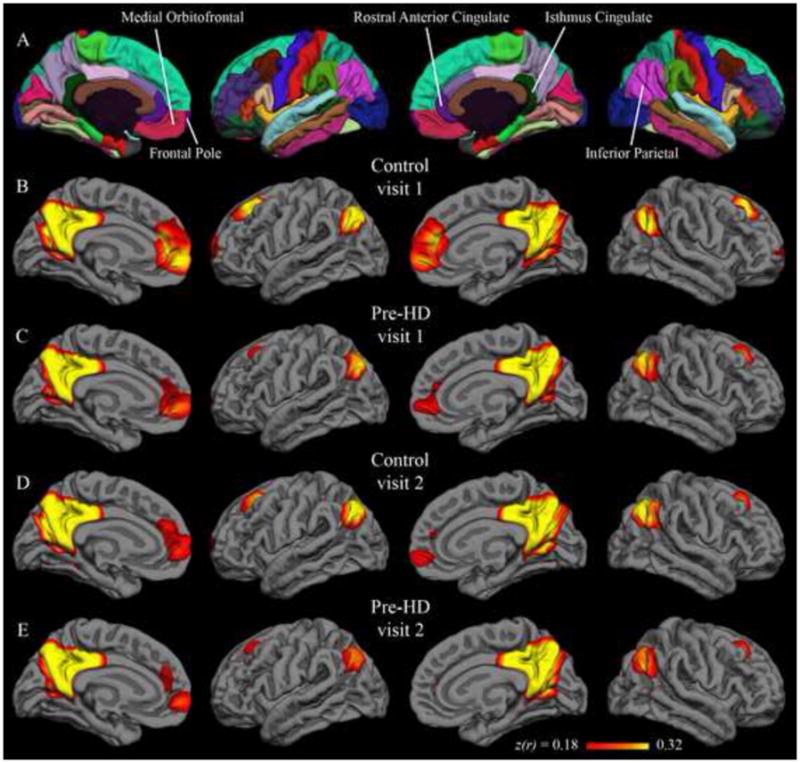
Group correlation maps with isthmus cingulate seed. Fisher’s z-transformed correlation coefficients for the correlation of each vertex on the surface with the average time series of the isthmus cingulate seed. The minimum and maximum thresholds for the functional overlay represent one and two standard deviations, respectively, above the mean coefficient from the first-visit group map for control subjects (i.e., Figure 1B). The top row (A) shows the Desikan-Killiany cortical parcellation atlas.

Figure 2.

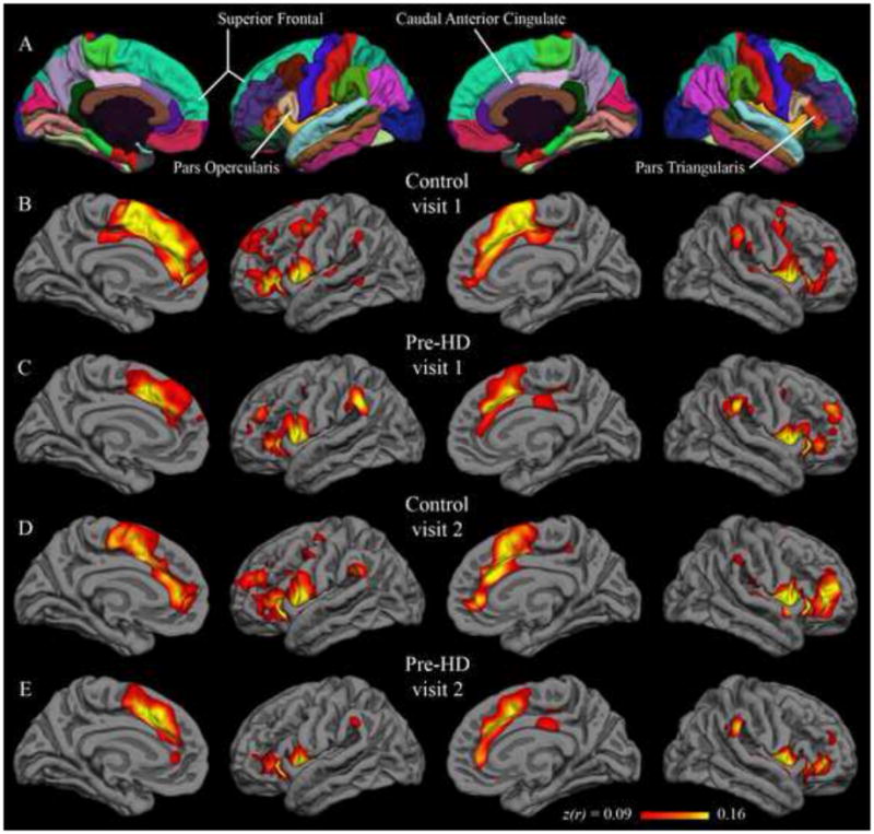
Group correlation maps with putamen seed. Fisher’s z-transformed correlation coefficients for the correlation of each vertex on the surface with the average time series of the putamen seed. The minimum and maximum thresholds for the functional overlay represent one and two standard deviations, respectively, above the mean coefficient from the first-visit group map for control subjects (i.e., Figure 2B). The top row (A) shows the Desikan-Killiany cortical parcellation atlas.

3.3 Stability of fMRI interregional correlations

Qualitative similarity of group-level results between visit 1 and visit 2 are confirmed by quantitative comparison. In the control group, the correlation between visit 1 and visit 2 isthmus cingulate results (correlation coefficient across all native-surface regions) was 0.93 in the left hemisphere and 0.90 in the right hemisphere. Pre-HD inter-visit correlations for the isthmus cingulate seed were also high, with coefficients of 0.96 in the left hemisphere and 0.94 in the right hemisphere. For the putamen seed, the control group visit 1 and visit 2 results had a correlation coefficient of 0.95 and 0.96 for the left and right hemispheres, respectively; the pre-HD group had values of 0.96 and 0.97 for the left and right hemispheres, respectively. Thus, group-level results for the native-surface parcellation regions were highly consistent for scans spaced a year apart.

Paired t-tests were applied to detect significant differences from visit 1 to visit 2. In the control group, with the isthmus cingulate seed, only the left rostral anterior cingulate region was significantly different after controlling for false discovery rate. The left rostral anterior cingulate had a group-mean z-transformed correlation coefficient of 0.46 at visit 1 and 0.24 at visit 2 (t(21) = 4.11; uncorrected p < 0.001). This rostral anterior cingulate finding was not replicated in the pre-HD group, though there was a trend in the same direction (0.36 at visit 1; 0.22 at visit 2; t(33) = 2.75; uncorrected p < 0.01). No region was significantly different from visit 1 to visit 2 in the pre-HD group for isthmus cingulate correlations. Likewise, no region showed a significant inter-visit difference in either group with the putamen seed. Vertex-wise paired t-test maps in Figure 3 (isthmus cingulate) and Figure 4 (putamen) also show very few significant inter-visit differences.

Figure 3.

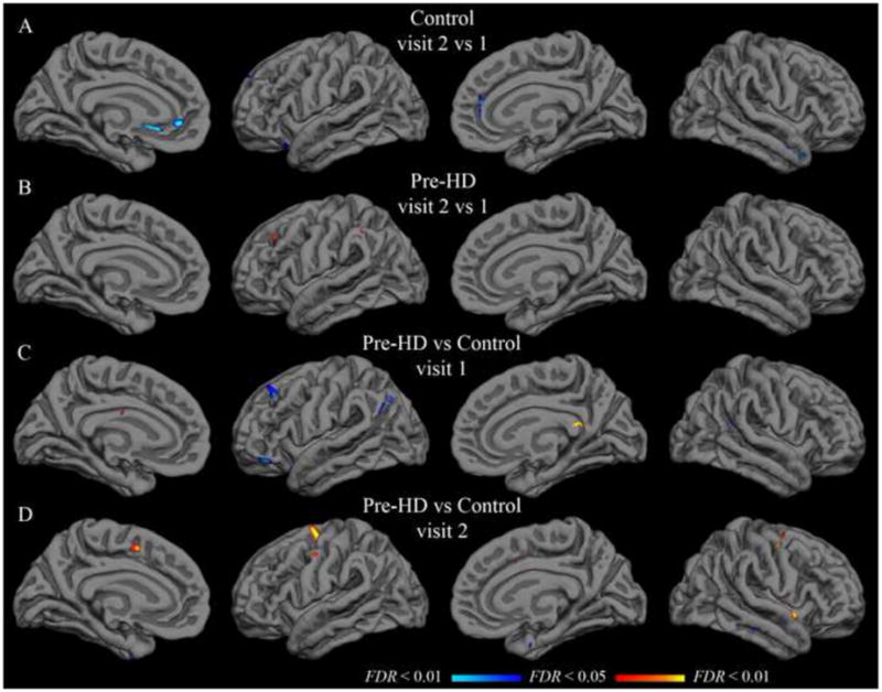
Group t-test maps with isthmus cingulate seed. Functional overlays show t-values for each vertex for the relevant comparison. The threshold for each row was set independently to indicate t-values corresponding to a false discovery rate less than 0.05 (minimum) and 0.01 (maximum). A–B: Hot colors indicate significantly greater correlation in visit 2; cool colors indicate significantly greater correlation in visit 1. C–D: Hot colors indicate greater correlation in the pre-HD group than in the control group; cool colors indicate greater correlation in the control group. Thresholds are as follows (min, max): (A) t = 3.6, 4.3; (B) t = 3.4, 4.0; (C–D) t = 3.3, 3.9.

Figure 4.

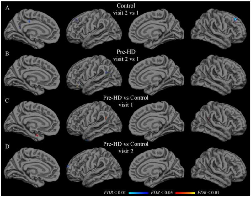
Group t-test maps with putamen seed. Functional overlays show t-values for each vertex for the relevant comparison. The threshold for each row was set independently to indicate t-values corresponding to a false discovery rate less than 0.05 (minimum) and 0.01 (maximum). A–B: Hot colors indicate significantly greater correlation in visit 2; cool colors indicate significantly greater correlation in visit 1. C–D: Hot colors indicate greater correlation in the pre-HD group than in the control group; cool colors indicate greater correlation in the control group. Thresholds are as follows (min, max): (A) t = 3.6, 4.3; (B) t = 3.4, 4.0; (C–D) t = 3.3, 3.9.

Power analyses were performed for each region to estimate the sample size necessary for 80% power to detect a difference of 0.2 in group mean correlation coefficient when alpha is set at 0.05. With the isthmus cingulate seed, the median calculated sample size (and interquartile range) across all regions was 21 (17–28) subjects for the control group and 25 (20–29) subjects for the pre-HD group. With the putamen seed, the median sample size was 21 (15–28) subjects for the control group and 22 (18–27) subjects for the pre-HD group. These estimates are comparable to the actual sample sizes of the present study.

While the correlation between visit 1 and visit 2 results was quite high at the group level, inter-visit correlation across native-surface regions was considerably lower for individual subjects. For control subjects, the median correlation coefficient between visit 1 and visit 2 with the isthmus cingulate seed was 0.59, with an interquartile range of 0.39–0.69. For pre-HD subjects, the median with the isthmus cingulate seed was 0.45, with an interquartile range of 0.21–0.59. With the putamen seed, the median (and interquartile range) for controls was 0.38 (0.17–0.60), and for pre-HD subjects was 0.51 (0.27–0.63).

Intraclass correlation coefficient analysis also suggested notable within-subjects variance from visit 1 to visit 2. ICC values for the regions from Tables 2 and 3 are shown in Tables 4 and 5, along with associated p-values. The greatest ICC with either seed was found in the right medial orbitofrontal region in the control group (ICC = 0.66, p < 0.001). ICC values significantly greater than zero (p < 0.05, uncorrected) with the isthmus cingulate seed were also found in the following regions in the control group: left cuneus, right rostral anterior cingulate, right frontal pole, and right superior frontal. In the pre-HD group, regions with ICC values significantly greater than zero with the isthmus cingulate seed included the left frontal pole, right medial orbitofrontal, and right inferior parietal. With the putamen seed, significant ICC values for the control group were found in right superior frontal and right caudal anterior cingulate regions. In the pre-HD group, the putamen seed gave significant ICC values in the left amygdala, right caudate, and right precentral regions. An ICC value greater than 0.5 indicates that between-subjects variance is greater than within-subjects variance. With the isthmus putamen seed, only the right medial orbitofrontal region had an ICC of at least 0.50 in both control and pre-HD groups. With the putamen seed, no region had an ICC of at least 0.50 in either group.

Table 4.

Intraclass correlation coefficients with isthmus cingulate seed. For easy comparison, regions are ordered according to the strength of correlation in the left hemisphere of the control group (see Table 2) for the other sub-tables. Intraclass correlation coefficients were calculated from visit 1 and visit 2 data from all subjects within each group. Significance is indicated by associated p-values (null hypothesis: ICC = 0).

CONTROL
LEFT HEMISPHERE			RIGHT HEMISPHERE
Region name	ICC	p	Region name	ICC	p
Medial Orbitofrontal	0.25	0.28	Medial Orbitofrontal	0.66	< 0.001
Rostral Anterior Cingulate	0.36	0.10	Rostral Anterior Cingulate	0.50	0.02
Frontal Pole	0.32	0.16	Frontal Pole	0.45	0.03
Inferior Parietal	0.12	0.61	Inferior Parietal	0.28	0.22
Superior Frontal	0.27	0.24	Superior Frontal	0.52	0.01
Cuneus	0.43	0.04	Cuneus	0.01	0.89
Hippocampus	0.24	0.29	Hippocampus	0.19	0.42

PRE-HD
LEFT HEMISPHERE			RIGHT HEMISPHERE
Region name	ICC	p	Region name	ICC	p
Medial Orbitofrontal	0.17	0.49	Medial Orbitofrontal	0.50	< 0.01
Rostral Anterior Cingulate	0.26	0.21	Rostral Anterior Cingulate	0.27	0.18
Frontal Pole	0.52	< 0.01	Frontal Pole	0.35	0.07
Inferior Parietal	0.23	0.28	Inferior Parietal	0.37	0.04
Superior Frontal	0.01	> 0.99	Superior Frontal	0.12	0.70
Cuneus	0.23	0.30	Cuneus	0.26	0.20
Hippocampus	0.07	0.91	Hippocampus	0.12	0.72

Table 5.

Intraclass correlation coefficients with putamen seed. For easy comparison, regions are ordered according to the strength of correlation in the left hemisphere of the control group (see Table 3) for the other sub-tables. Intraclass correlation coefficients were calculated from visit 1 and visit 2 data from all subjects within each group. Significance is indicated by associated p-values (null hypothesis: ICC = 0).

CONTROL
LEFT HEMISPHERE			RIGHT HEMISPHERE
Region name	ICC	p	Region name	ICC	p
Caudate	0.11	0.63	Caudate	0.30	0.18
Superior Frontal	0.00	0.90	Superior Frontal	0.47	0.02
Pars Triangularis	< 0.01	0.90	Pars Triangularis	0.16	0.49
Pars Opercularis	< 0.01	0.90	Pars Opercularis	0.01	0.88
Precentral	0.10	0.67	Precentral	0.30	0.18
Amygdala	0.04	0.83	Amygdala	0.20	0.40
Caudal Anterior Cingulate	0.23	0.32	Caudal Anterior Cingulate	0.52	0.01

PRE-HD
LEFT HEMISPHERE			RIGHT HEMISPHERE
Region name	ICC	p	Region name	ICC	p
Caudate	0.32	0.10	Caudate	0.49	< 0.01
Superior Frontal	< 0.01	> 0.99	Superior Frontal	< 0.01	> 0.99
Pars Triangularis	0.20	0.37	Pars Triangularis	0.16	0.55
Pars Opercularis	0.01	> 0.99	Pars Opercularis	< 0.01	> 0.99
Precentral	0.28	0.16	Precentral	0.42	0.02
Amygdala	0.38	0.04	Amygdala	0.15	0.59
Caudal Anterior Cingulate	0.22	0.33	Caudal Anterior Cingulate	0.25	0.23

3.4 Effect of pre-HD on interregional correlations

Population mean correlations with the isthmus cingulate seed for pre-HD and control groups did not differ significantly in any of the native-surface regions in either hemisphere at visit 1 (two-sample t-tests, FDR controlled at less than 0.05). This remained true approximately one year later at visit 2. Likewise, no statistically significant difference was found for correlation with the putamen seed in any of the parcellation regions at either visit. Vertex-wise t-tests on the group surface also yielded only sparse spots showing significant effects of pre-HD with either seed (Figures 3 and 4).

Though the change from visit 1 to visit 2 was unimpressive at the group level for either population, the size of the longitudinal change in pre-HD might still differ from controls in some region(s). However, two-sample t-tests comparing the visit 2 - visit 1 difference in pre-HD subjects to that of control subjects did not yield any native-surface parcellation regions with a statistically significant effect. This was true with both the isthmus cingulate and putamen seeds. Vertex-wise t-tests on the group surface were consistent with the native-surface region results (Figure 5 in Supplementary Materials).

Comparison of interregional correlations with indicators of disease severity in the pre-HD group did not reveal any associations for the isthmus cingulate seed correlations (results not shown), but potential associations were identified for the putamen seed correlations (Table 6). Subjects with weaker putamen-caudate functional correlation at visit 1 were also closer to disease onset using the Langbehn method. This was true in each hemisphere. Similarly, subjects with weaker putamen-caudate functional correlation at visit 1 also had smaller caudate and putamen volumes (Table 6). These findings were less consistent at visit 2, though trends in the same direction remained.

Table 6.

Association of putamen functional correlations with disease severity. Regions most strongly correlated with the putamen seed in the control group are included in the table. YTO: years to onset; r: Pearson’s correlation coefficient.

Putamen-Region Correlation vs. Years to Onset
Region name	Visit 1				Visit 2
	Langbehn YTO		Aylward YTO		Langbehn YTO		Aylward YTO
	r	p	r	p	r	p	r	p
Left Caudate	0.54**	< 0.01	0.16	0.37	0.30†	0.08	0.28	0.11
Left Pars Opercularis	0.07	0.71	−0.08	0.67	0.06	0.72	−0.13	0.46
Left Superior Frontal	−0.17	0.35	−0.34†	0.05	−0.09	0.62	0.03	0.87
Right Caudate	0.41*	0.02	0.17	0.34	0.24	0.17	0.32†	0.07
Right Pars Opercularis	0.21	0.24	−0.06	0.76	0.09	0.62	−0.01	0.96
Right Superior Frontal	0.04	0.81	−0.23	0.19	0.15	0.40	0.09	0.62

Putamen-Region Correlation vs. Striatal Volume
Region name	Visit 1				Visit 2
	Caudate Volume		Putamen Volume		Caudate Volume		Putamen Volume
	r	p	r	p	r	p	r	p
Left Caudate	0.36**	< 0.01	0.31*	0.02	0.37*	0.03	0.29†	0.09
Left Pars Opercularis	−0.09	0.50	−0.05	0.71	−0.08	0.67	−0.13	0.47
Left Superior Frontal	< 0.01	0.99	0.09	0.50	−0.10	0.56	−0.13	0.47
Right Caudate	0.27*	0.04	0.23†	0.09	0.24	0.18	0.22	0.22
Right Pars Opercularis	−0.02	0.89	0.03	0.85	0.11	0.55	0.05	0.77
Right Superior Frontal	0.06	0.65	0.16	0.25	−0.08	0.68	−0.03	0.86

^**p < 0.01

^*p < 0.05

^†p < 0.10

4 Discussion

In assessing the potential of resting correlations as a biomarker, the primary objectives of the present study were to evaluate the long-term stability of measures obtained in native space and to apply the technique to the premanifest HD population. Group correlation results obtained using the native-surface method highlighted corticostriatal and default patterns that were stable over one year in both the control and pre-HD populations. On the other hand, results from visit 1 and visit 2 were less stable at the individual-subject level. No significant group-level differences were demonstrated between the pre-HD and control groups, but weakening of resting correlation between the caudate and putamen in the pre-HD group may be related to disease severity as estimated by subcortical volumes or estimated years to symptom onset.

4.1 Isthmus cingulate and putamen seeds yield expected networks

Regions with strongest correlation with the isthmus and putamen seeds were consistent with previously published group-level resting fMRI results. Specifically, the isthmus cingulate seed highlighted default network areas such as dorsolateral prefrontal, medial prefrontal, inferior parietal, and medial temporal cortex bilaterally in both the control group and the pre-HD group (Table 2, Figure 1). The putamen seed, on the other hand, was most strongly correlated with motor-related areas (Table 3, Figure 2) in both populations. Distinguishable patterns with these two seeds converges with prior studies demonstrating dissociable “networks” of brain regions at rest (Beckmann et al., 2005; Seeley et al., 2009; Vincent et al., 2007) and, along with supplementary analyses using the caudate seed, are further evidence that seeds defined by automated parcellation on the native surface yield meaningful and reproducible results. Consistent with known structural connectivity (Alexander et al., 1986; Lawrence et al., 1998; Leh et al., 2007), the caudate maps differ from those using the putamen seed, highlighting dorsolateral prefrontal and anterior cingulate cortex, whereas the putamen maps highlight ventrolateral prefrontal cortex and supplementary motor area (Figure 6 in Supplementary Materials). Also of note, the magnitudes of the isthmus cingulate correlations are generally greater than that of the putamen (or caudate) correlations. While this confirms multiple previous findings that the default network is particularly active at rest (Buckner et al., 2008; Greicius et al., 2003; Raichle et al., 2001), it also suggests a resting condition may not be optimal for studies specifically focused on corticostriatal networks. Resting correlations in this study did, however, highlight both corticostriatal and default networks in four data sets (two populations at two time points).

4.2 Resting interregional correlations stable over one year at group level

Group-level results with both putamen and isthmus cingulate seeds were longitudinally stable, yielding similar patterns in scans collected a year apart. Qualitatively similar group maps (Figures 1–2) and native-surface results (Tables 2–3) are corroborated by strong inter-visit correlations at the group level (greater than 0.9 in each hemisphere in all four data sets). Additionally, only a single region, in a single group, showed a statistical difference between visit 1 and visit 2. The congruency of group results from data collected a year apart is encouraging for application of this technique to longitudinal studies such as clinical trials. That this relatively high long-term stability held in both control and pre-HD populations is also encouraging, as it suggests population differences could also be consistently measured over a year-long study.

Subject-level results were considerably less stable than group-level results from visit 1 to visit 2. Inter-visit correlations at the subject level had medians of 0.59 and 0.45 for the isthmus cingulate seed (left and right hemispheres), and 0.38 and 0.51 for the putamen seed. While there is still reasonable inter-visit agreement for many subjects (approximately 25% of subjects in each group had inter-visit correlations greater than 0.60), the within-subjects variance is approximately as great, or greater, than the between-subjects variance in nearly every case. In other words, for a given single region, on average, measurements taken from the same individual a year apart were at least as different as measurements taken from two different individuals from within the same group.

Strong group-level stability with high within-subjects variance is suggestive of a noisy marker that can be consistent at the group level because of improved signal-to-noise ratio with averaging. The sources of this noise may be varied. Technical imaging issues may contribute, including fluctuations in scanner properties, thermal noise, physiological noise (e.g., due to changes in respiration), and static field distortions. Additionally, different scan sessions might have involved different levels of anxiety, alertness, mood, fatigue, or mental activities. It is also unknown to what extent the physiological phenomenon underlying interregional BOLD correlations is stable in the absence of all measurement noise. The strength of these resting BOLD correlations may naturally fluctuate over time; in fact, coherence analysis has provided evidence for such fluctuation even within a single scan (Chang and Glover, 2010). Despite the apparently high noise, the stable group results indicate that efforts to minimize measurement noise and account for biological variation might improve the reproducibility of resting fMRI results in individual subjects.

4.3 Resting interregional correlations only modestly affected in premanifest stage

Premanifest Huntington’s disease did not greatly disrupt interregional BOLD correlations in the present study. Functional correlations for the pre-HD group were compared to age-matched controls with two different seeds and at two different time points. The lack of difference in fMRI correlations was found despite reliable genetic diagnosis and measured structural differences on MRI in the same subjects (Majid et al., 2011). It is possible there is an underlying effect of pre-HD, but the present results suggest it would be relatively small. Power analyses (Tables 2–3) estimate the present sample sizes are sufficient for fairly high power to detect an effect size of 0.2 in most regions, a conservative value selected to detect an effect even in studies including healthy subjects at high-risk of other neurodegenerative diseases (Fleisher et al., 2009; Hedden et al., 2009; Koch et al., 2010). Power in the present study to detect a population difference was even higher because the initial comparison was repeated in a second set of measurements (visit 2). If there are subtle effects of pre-HD on interregional BOLD correlations, these might be detected with improved signal-to-noise ratio or larger sample sizes. However, in light of the present results, other potential biomarkers might be more sensitive to premanifest Huntington’s pathology than resting fMRI correlations (Aylward et al., 1996; Majid et al., 2011; Tabrizi et al., 2011).

It is also possible that resting fMRI correlations differ with pre-HD when some other region is selected as the seed. No standard way exists to determine which, or even how many, seeds to use. One approach would be to repeat the full, whole-brain analysis with each of the 80 regions, in turn, as the seed. Another would be to try each vertex of the group surface as a seed, though spatial smoothness, alone, implies this approach entails redundancy. The sensitivity of these exploratory approaches is high, but this sensitivity comes at the cost of a potentially steep decrease in statistical power due to a dramatically larger multiple comparisons problem. In the present experiment we have opted to focus on two anatomical seeds that were selected a priori based on existing functional and pathological evidence.

The paucity of significant differences in resting correlations between pre-HD and control groups may be unsurprising given that cognition is relatively intact and motor symptoms have not yet manifested at this early stage of the disease. While structural changes in these subjects brains suggest disease progression, these changes may still be insufficient to overcome subjects functional reserve. As gene-positive individuals begin to experience cognitive impairment, resting BOLD correlations may also become disrupted. Indeed, the within-group associations with disease severity shown in Table 6 suggest that disease progression might affect functional correlations between the caudate and putamen, even in the premanifest stage.

4.4 Methodological considerations

As the surface-based analysis methods used here are relatively new, and therefore less common than analyses based on volume-atlas transformation, a brief treatment of its implications may be warranted; for more complete discussion, the reader is referred to Seibert and Brewer (2011). First, native-space parcellation analysis represents a spatial reduction of the data from thousands of voxels to approximately 80 regions. In addition to reducing multiple comparisons and focusing on voxels within the gray matter, this step increases signal-to-noise ratio by averaging neighboring cortical data points. Most importantly, this parcellation allows across-subject or across-group comparisons of measurements made in native space. However, a limitation of the parcellation regions is dependence on anatomical regions that may have an imperfect correspondence with functional regions in the brain, and so vertex-wise analysis was also performed on a common group surface. This complementary analysis is useful for identifying any functional features of the data that conform poorly to anatomical regions, as well as for visualizing group-level results.

Native-surface parcellation and surface-based registration may not completely remove all effects of anatomic variability, but they still have important advantages over methods based on transformation to a volume atlas. In particular, the accuracy of surface generation—the step that determines whether cortical gray matter is correctly identified—is easily evaluated by visual inspection on a slice-by-slice basis (a processed described in more detail in FreeSurfer documentation and in Seibert and Brewer, 2011). A primary concern with volume-atlas analysis is that individuals cerebrospinal fluid and white matter may be interpreted as gray matter in atlas space (and vice versa) due to small, local registration errors that can be widespread and difficult to identify or correct. These errors are more readily avoided in the surface-based methods because tissue segmentation is performed, inspected, and, if necessary, manually corrected using the native images. It has already been demonstrated by direct comparison that the single step of registration to a volume atlas can introduce large changes in resting fMRI correlations (Seibert and Brewer, 2011).

4.5 Future directions

Efforts could be made in future studies to attempt to address limitations of resting fMRI suggested by the present study. The most important limitation is probably the signal-to-noise ratio of the resting BOLD correlations. As intimated above, improvements in scanner stability and technical aspects of functional imaging might lead to increases in signal-to-noise ratio. Though potential changes in hardware performance over time did not introduce significant systematic changes to group-level fMRI results in the present data, the possibility of such changes should be considered in future studies. Additionally, physiological noise arising from fluctuations in heart rate or respiration might be somewhat better controlled if these metrics were measured and their effects modeled (Glover et al., 2000). Rigorous investigation might also be directed toward achieving an optimal scanning environment to produce more homogeneity in the “resting” condition of the subjects; this could include instructions regarding the mental activities subjects should engage in or avoid, the illumination of the room, subject comfort in the scanner, whether visual fixation is encouraged, and many other considerations. Correlation measures have been shown to be fairly consistent with four-minute resting scans (Van Dijk et al., 2009; Whitlow et al., 2011), and the six-minute scans used here are within the typical range for resting fMRI; however, increased scan duration might still improve signal-to-noise ratio and possibly improve stability of individual-subject measurements. Finally, recent work has shown that some graph theory metrics of resting fMRI data are relatively consistent with as little as two minutes of data, suggesting such global network measures may prove more useful in individual subjects (Whitlow et al., 2011; Petrella, 2011).

Supplementary Material

01. Figure 5.

Longitudinal group t-test maps. Functional overlays show t-values for each vertex for the relevant comparison. The thresholds were set to indicate t-values corresponding to a false discovery rate less than 0.05 (minimum) and 0.01 (maximum). A–B: Hot colors indicate significantly greater longitudinal change in pre-HD subjects than in control subjects; cool colors indicate greater longitudinal change in control subjects. Thresholds are (min, max): t = 3.3, 3.9.

02. Figure 6.

Group correlation maps with caudate seed. Fisher’s z-transformed correlation coefficients for the correlation of each vertex on the surface with the average time series of the caudate seed. The minimum and maximum thresholds for the functional overlay represent one and two standard deviations, respectively, above the mean coefficient from the first-visit group map for control subjects (i.e., Figure 2B). The top row (A) shows the Desikan-Killiany cortical parcellation atlas.

Highlights.

• Test-retest resting fMRI scans one year apart in healthy adults and pre-HD

• Resting BOLD correlations show good longitudinal stability over one year

• Analysis in native space to avoid confounds from misregistration to standard space

• Pre-HD has only modest effects on resting BOLD correlations

Abbreviations

BOLD

blood oxygenation level dependent

fMRI

functional magnetic resonance imaging

HD

Huntington’s disease

pre-HD

premanifest Huntington’s disease

MNI

Montreal Neurological Institute

ICC

intraclass correlation coefficient

MMSE

mini-mental state exam

CAG

cytosine-adenine-guanine

UHDRS

Unified Huntington’s Disease Rating Scale

References

- Alexander GE, DeLong MR, Strick PL. Parallel organization of functionally segregated circuits linking basal ganglia and cortex. Annu Rev Neurosci. 1986;9:357–381. doi: 10.1146/annurev.ne.09.030186.002041. [DOI] [PubMed] [Google Scholar]
- Auer DP. Spontaneous low-frequency blood oxygenation level-dependent fluctuations and functional connectivity analysis of the “resting” brain. Magn Reson Imaging. 2008;26(7):1055–1064. doi: 10.1016/j.mri.2008.05.008. [DOI] [PubMed] [Google Scholar]
- Aylward EH, Sparks BF, Field KM, Yallapragada V, Shpritz BD, Rosenblatt A, et al. Onset and rate of striatal atrophy in preclinical Huntington disease. Neurology. 2004;63(1):66–72. doi: 10.1212/01.wnl.0000132965.14653.d1. Retrieved May 18, 2011. [DOI] [PubMed] [Google Scholar]
- Aylward EH, Codori AM, Barta PE, Pearlson GD, Harris GJ, Brandt J. Basal ganglia volume and proximity to onset in presymptomatic Huntington disease. Arch Neurol. 1996;53(12):1293–1296. doi: 10.1001/archneur.1996.00550120105023. Retrieved May 6, 2011. [DOI] [PubMed] [Google Scholar]
- Aylward EH, Nopoulos PC, Ross CA, Langbehn DR, Pierson RK, Mills JA, et al. Longitudinal change in regional brain volumes in prodromal Huntington disease. J Neurol Neurosurg Psychiatr. 2011;82(4):405–410. doi: 10.1136/jnnp.2010.208264. [DOI] [PMC free article] [PubMed] [Google Scholar]
- Bai F, Watson DR, Yu H, Shi Y, Yuan Y, Zhang Z. Abnormal resting-state functional connectivity of posterior cingulate cortex in amnestic type mild cognitive impairment. Brain Res. 2009;1302:167–174. doi: 10.1016/j.brainres.2009.09.028. [DOI] [PubMed] [Google Scholar]
- Beckmann CF, DeLuca M, Devlin JT, Smith SM. Investigations into resting-state connectivity using independent component analysis. Philos Trans R Soc Lond, B, Biol Sci. 2005;360(1457):1001–1013. doi: 10.1098/rstb.2005.1634. [DOI] [PMC free article] [PubMed] [Google Scholar]
- Biswal B, Yetkin FZ, Haughton VM, Hyde JS. Functional connectivity in the motor cortex of resting human brain using echo-planar MRI. Magn Reson Med. 1995;34(4):537–541. doi: 10.1002/mrm.1910340409. [DOI] [PubMed] [Google Scholar]
- Bohanna I, Georgiou-Karistianis N, Hannan AJ, Egan GF. Magnetic resonance imaging as an approach towards identifying neuropathological biomarkers for Huntington’s disease. Brain Res Rev. 2008;58(1):209–225. doi: 10.1016/j.brainresrev.2008.04.001. [DOI] [PubMed] [Google Scholar]
- Buckner RL, Andrews-Hanna JR, Schacter DL. The Brain’s Default Network: Anatomy, Function, and Relevance to Disease. Annals of the New York Academy of Sciences. 2008;1124(1):1–38. doi: 10.1196/annals.1440.011. [DOI] [PubMed] [Google Scholar]
- Chang C, Glover GH. Time-frequency dynamics of resting-state brain connectivity measured with fMRI. Neuroimage. 2010;50(1):81–98. doi: 10.1016/j.neuroimage.2009.12.011. [DOI] [PMC free article] [PubMed] [Google Scholar]
- Chen S, Ross TJ, Zhan W, Myers CS, Chuang K-S, Heishman SJ, Stein EA, Yang Y. Group independent component analysis reveals consistent resting-state networks across multiple sessions. Brain Res. 2008;1239:141–151. doi: 10.1016/j.brainres.2008.08.028. [DOI] [PMC free article] [PubMed] [Google Scholar]
- Cohen J. Statistical power analysis for the behavioral sciences. 2. Psychology Press; 1988. [Google Scholar]
- Cox RW, Jesmanowicz A. Real-time 3D image registration for functional MRI. Magn Reson Med. 1999;42(6):1014–1018. doi: 10.1002/(sici)1522-2594(199912)42:6<1014::aid-mrm4>3.0.co;2-f. Retrieved November 2, 2010. [DOI] [PubMed] [Google Scholar]
- Dale AM, Fischl B, Sereno MI. Cortical surface-based analysis. I. Segmentation and surface reconstruction. Neuroimage. 1999;9(2):179–194. doi: 10.1006/nimg.1998.0395. [DOI] [PubMed] [Google Scholar]
- Damoiseaux JS, Rombouts SARB, Barkhof F, Scheltens P, Stam CJ, Smith SM, Beckmann CF. Consistent resting-state networks across healthy subjects. Proc Natl Acad Sci USA. 2006;103(37):13848–13853. doi: 10.1073/pnas.0601417103. [DOI] [PMC free article] [PubMed] [Google Scholar]
- Dawson B, Trapp RG. Basic & clinical biostatistics. 4. Lange Medical Books/McGraw-Hill; 2004. [Google Scholar]
- Desikan RS, Ségonne F, Fischl B, Quinn BT, Dickerson BC, Blacker D, et al. An automated labeling system for subdividing the human cerebral cortex on MRI scans into gyral based regions of interest. Neuroimage. 2006;31(3):968–980. doi: 10.1016/j.neuroimage.2006.01.021. [DOI] [PubMed] [Google Scholar]
- Eidelberg D, Surmeier DJ. Brain networks in Huntington disease. J Clin Invest. 2011;121(2):484–492. doi: 10.1172/JCI45646. [DOI] [PMC free article] [PubMed] [Google Scholar]
- Fischl B, van der Kouwe A, Destrieux C, Halgren E, Segonne F, Salat DH, et al. Automatically Parcellating the Human Cerebral Cortex. Cereb Cortex. 2004;14(1):11–22. doi: 10.1093/cercor/bhg087. [DOI] [PubMed] [Google Scholar]
- Fischl B, Salat DH, Busa E, Albert M, Dieterich M, Haselgrove C, et al. Neuron. 3. Vol. 33. 2002. Whole brain segmentation: automated labeling of neuroanatomical structures in the human brain; pp. 341–355. Retrieved November 2, 2010. [DOI] [PubMed] [Google Scholar]
- Fischl B, Sereno MI, Dale AM. Cortical surface-based analysis. II: Inflation, flattening, and a surface-based coordinate system. Neuroimage. 1999a;9(2):195–207. doi: 10.1006/nimg.1998.0396. [DOI] [PubMed] [Google Scholar]
- Fischl B, Sereno MI, Tootell RB, Dale AM. High-resolution intersubject averaging and a coordinate system for the cortical surface. Hum Brain Mapp. 1999b;8(4):272–284. doi: 10.1002/(SICI)1097-0193(1999)8:4<272::AID-HBM10>3.0.CO;2-4. Retrieved July 29, 2009. [DOI] [PMC free article] [PubMed] [Google Scholar]
- Fleisher AS, Sherzai A, Taylor C, Langbaum JBS, Chen K, Buxton RB. Resting-state BOLD networks versus task-associated functional MRI for distinguishing Alzheimer’s disease risk groups. Neuroimage. 2009;47(4):1678–1690. doi: 10.1016/j.neuroimage.2009.06.021. [DOI] [PMC free article] [PubMed] [Google Scholar]
- Folstein MF, Folstein SE, McHugh PR. “Mini-mental state”. A practical method for grading the cognitive state of patients for the clinician. J Psychiatr Res. 1975;12(3):189–198. doi: 10.1016/0022-3956(75)90026-6. Retrieved May 6, 2011. [DOI] [PubMed] [Google Scholar]
- Fox MD, Raichle ME. Spontaneous fluctuations in brain activity observed with functional magnetic resonance imaging. Nat Rev Neurosci. 2007;8(9):700–11. doi: 10.1038/nrn2201. [DOI] [PubMed] [Google Scholar]
- Genovese CR, Lazar NA, Nichols T. Thresholding of Statistical Maps in Functional Neuroimaging Using the False Discovery Rate. NeuroImage. 2002;15(4):870–878. doi: 10.1006/nimg.2001.1037. [DOI] [PubMed] [Google Scholar]
- Glover GH, Li TQ, Ress D. Image-based method for retrospective correction of physiological motion effects in fMRI: RETROICOR. Magn Reson Med. 2000;44(1):162–167. doi: 10.1002/1522-2594(200007)44:1<162::aid-mrm23>3.0.co;2-e. Retrieved October 2, 2009. [DOI] [PubMed] [Google Scholar]
- Greicius MD, Krasnow B, Reiss AL, Menon V. Functional connectivity in the resting brain: a network analysis of the default mode hypothesis. Proc Natl Acad Sci USA. 2003;100(1):253–258. doi: 10.1073/pnas.0135058100. [DOI] [PMC free article] [PubMed] [Google Scholar]
- Greicius MD. Resting-state functional connectivity in neuropsychiatric disorders. Curr Opin Neurol. 2008;21(4):424–430. doi: 10.1097/WCO.0b013e328306f2c5. [DOI] [PubMed] [Google Scholar]
- Greicius MD, Srivastava G, Reiss AL, Menon V. Default-mode network activity distinguishes Alzheimer’s disease from healthy aging: evidence from functional MRI. Proc Natl Acad Sci USA. 2004;101(13):4637–4642. doi: 10.1073/pnas.0308627101. [DOI] [PMC free article] [PubMed] [Google Scholar]
- Harris GJ, Pearlson GD, Peyser CE, Aylward EH, Roberts J, Barta PE, Chase GA, Folstein SE. Putamen volume reduction on magnetic resonance imaging exceeds caudate changes in mild Huntington’s disease. Ann Neurol. 1992;31(1):69–75. doi: 10.1002/ana.410310113. [DOI] [PubMed] [Google Scholar]
- Hedden T, Van Dijk KRA, Becker JA, Mehta A, Sperling RA, Johnson KA, Buckner RL. Disruption of functional connectivity in clinically normal older adults harboring amyloid burden. J Neurosci. 2009;29(40):12686–12694. doi: 10.1523/JNEUROSCI.3189-09.2009. [DOI] [PMC free article] [PubMed] [Google Scholar]
- Helmich RC, Derikx LC, Bakker M, Scheeringa R, Bloem BR, Toni I. Spatial remapping of cortico-striatal connectivity in Parkinson’s disease. Cereb Cortex. 2010;20(5):1175–1186. doi: 10.1093/cercor/bhp178. [DOI] [PubMed] [Google Scholar]
- van den Heuvel MP, Hulshoff Pol HE. Exploring the brain network: A review on resting-state fMRI functional connectivity. European Neuropsychopharmacology. 2010;20(8):519–534. doi: 10.1016/j.euroneuro.2010.03.008. [DOI] [PubMed] [Google Scholar]
- Huntington Study Group. Unified Huntington’s Disease Rating Scale: reliability and consistency. Huntington Study Group. Mov Disord. 1996;11(2):136–142. doi: 10.1002/mds.870110204. [DOI] [PubMed] [Google Scholar]
- Jafri MJ, Pearlson GD, Stevens M, Calhoun VD. A method for functional network connectivity among spatially independent resting-state components in schizophrenia. Neuroimage. 2008;39(4):1666–1681. doi: 10.1016/j.neuroimage.2007.11.001. [DOI] [PMC free article] [PubMed] [Google Scholar]
- Klöppel S, Henley SM, Hobbs NZ, Wolf RC, Kassubek J, Tabrizi SJ, Frackowiak RSJ. Magnetic resonance imaging of Huntington’s disease: preparing for clinical trials. Neuroscience. 2009;164(1):205–219. doi: 10.1016/j.neuroscience.2009.01.045. [DOI] [PMC free article] [PubMed] [Google Scholar]
- Koch W, Teipel S, Mueller S, Benninghoff J, Wagner M, Bokde ALW, et al. Diagnostic power of default mode network resting state fMRI in the detection of Alzheimer’s disease. Neurobiol Aging. 2010 doi: 10.1016/j.neurobiolaging.2010.04.013. [DOI] [PubMed] [Google Scholar]
- Krishnan S, Slavin MJ, Tran T-TT, Doraiswamy PM, Petrella JR. Accuracy of spatial normalization of the hippocampus: implications for fMRI research in memory disorders. Neuroimage. 2006;31(2):560–571. doi: 10.1016/j.neuroimage.2005.12.061. [DOI] [PubMed] [Google Scholar]
- Langbehn DR, Brinkman RR, Falush D, Paulsen JS, Hayden MR. A new model for prediction of the age of onset and penetrance for Huntington’s disease based on CAG length. Clin Genet. 2004;65(4):267–277. doi: 10.1111/j.1399-0004.2004.00241.x. [DOI] [PubMed] [Google Scholar]
- Lawrence AD, Sahakian BJ, Robbins TW. Cognitive functions and corticostriatal circuits: insights from Huntington’s disease. Trends Cogn Sci (Regul Ed) 1998;2(10):379–388. doi: 10.1016/s1364-6613(98)01231-5. Retrieved May 6, 2011. [DOI] [PubMed] [Google Scholar]
- Leh SE, Ptito A, Chakravarty MM, Strafella AP. Fronto-striatal connections in the human brain: a probabilistic diffusion tractography study. Neurosci Lett. 2007;419(2):113–118. doi: 10.1016/j.neulet.2007.04.049. [DOI] [PMC free article] [PubMed] [Google Scholar]
- Majid DSA, Stoffers D, Sheldon S, Hamza S, Thompson WK, Goldstein J, Corey-Bloom J, Aron AR. Automated structural imaging analysis detects premanifest Huntington’s disease neurodegeneration within 1 year. Mov Disord. 2011 doi: 10.1002/mds.23656. [DOI] [PMC free article] [PubMed] [Google Scholar]
- Meindl T, Teipel S, Elmouden R, Mueller S, Koch W, Dietrich O, Coates U, Reiser M, Glaser C. Test-retest reproducibility of the default-mode network in healthy individuals. Hum Brain Mapp. 2010;31(2):237–246. doi: 10.1002/hbm.20860. [DOI] [PMC free article] [PubMed] [Google Scholar]
- Mohammadi B, Kollewe K, Samii A, Beckmann CF, Dengler R, Münte TF. Changes in resting-state brain networks in writer’s cramp. Hum Brain Mapp. 2011a doi: 10.1002/hbm.21250. [DOI] [PMC free article] [PubMed] [Google Scholar]
- Mohammadi B, Kollewe K, Samii A, Dengler R, Münte TF. Functional neuroimaging at different disease stages reveals distinct phases of neuroplastic changes in amyotrophic lateral sclerosis. Hum Brain Mapp. 2011b;32(5):750–758. doi: 10.1002/hbm.21064. [DOI] [PMC free article] [PubMed] [Google Scholar]
- Paulsen JS, Nopoulos PC, Aylward E, Ross CA, Johnson H, Magnotta VA, et al. Striatal and white matter predictors of estimated diagnosis for Huntington disease. Brain Res Bull. 2010;82(3–4):201–207. doi: 10.1016/j.brainresbull.2010.04.003. [DOI] [PMC free article] [PubMed] [Google Scholar]
- Paulsen JS, Zimbelman JL, Hinton SC, Langbehn DR, Leveroni CL, Benjamin ML, Reynolds NC, Rao SM. fMRI biomarker of early neuronal dysfunction in presymptomatic Huntington’s Disease. AJNR Am J Neuroradiol. 2004;25(10):1715–1721. Retrieved May 6, 2011. [PMC free article] [PubMed] [Google Scholar]
- Petrella JR. Use of Graph Theory to Evaluate Brain Networks: A Clinical Tool for a Small World? Radiology. 2011;259(2):317–320. doi: 10.1148/radiol.11110380. [DOI] [PubMed] [Google Scholar]
- Pihlajamäki M, Jauhiainen AM, Soininen H. Structural and functional MRI in mild cognitive impairment. Curr Alzheimer Res. 2009;6(2):179–185. doi: 10.2174/156720509787602898. Retrieved August 27, 2009. [DOI] [PubMed] [Google Scholar]
- Raichle ME, MacLeod AM, Snyder AZ, Powers WJ, Gusnard DA, Shulman GL. A default mode of brain function. Proc Natl Acad Sci USA. 2001;98(2):676–682. doi: 10.1073/pnas.98.2.676. [DOI] [PMC free article] [PubMed] [Google Scholar]
- Reading SAJ, Dziorny AC, Peroutka LA, Schreiber M, Gourley LM, Yallapragada V, et al. Functional brain changes in presymptomatic Huntington’s disease. Ann Neurol. 2004;55(6):879–883. doi: 10.1002/ana.20121. [DOI] [PubMed] [Google Scholar]
- Repovs G, Csernansky JG, Barch DM. Brain network connectivity in individuals with schizophrenia and their siblings. Biol Psychiatry. 2011;69(10):967–973. doi: 10.1016/j.biopsych.2010.11.009. [DOI] [PMC free article] [PubMed] [Google Scholar]
- Rogers BP, Morgan VL, Newton AT, Gore JC. Assessing functional connectivity in the human brain by fMRI. Magn Reson Imaging. 2007;25(10):1347–1357. doi: 10.1016/j.mri.2007.03.007. [DOI] [PMC free article] [PubMed] [Google Scholar]
- Rosas HD, Feigin AS, Hersch SM. Using advances in neuroimaging to detect, understand, and monitor disease progression in Huntington’s disease. NeuroRx. 2004;1(2):263–272. doi: 10.1602/neurorx.1.2.263. Retrieved May 19, 2011. [DOI] [PMC free article] [PubMed] [Google Scholar]
- Rosas HD, Salat DH, Lee SY, Zaleta AK, Hevelone N, Hersch SM. Complexity and heterogeneity: what drives the ever-changing brain in Huntington’s disease? Ann N Y Acad Sci. 2008;1147:196–205. doi: 10.1196/annals.1427.034. [DOI] [PMC free article] [PubMed] [Google Scholar]
- Seeley WW, Crawford RK, Zhou J, Miller BL, Greicius MD. Neurodegenerative diseases target large-scale human brain networks. Neuron. 2009;62(1):42–52. doi: 10.1016/j.neuron.2009.03.024. [DOI] [PMC free article] [PubMed] [Google Scholar]
- Seibert TM, Brewer JB. Default network correlations analyzed on native surfaces. J Neurosci Methods. 2011 doi: 10.1016/j.jneumeth.2011.04.010. [DOI] [PMC free article] [PubMed] [Google Scholar]
- Shehzad Z, Kelly AMC, Reiss PT, Gee DG, Gotimer K, Uddin LQ, et al. The resting brain: unconstrained yet reliable. Cereb Cortex. 2009;19(10):2209–2229. doi: 10.1093/cercor/bhn256. [DOI] [PMC free article] [PubMed] [Google Scholar]
- Sheline YI, Raichle ME, Snyder AZ, Morris JC, Head D, Wang S, Mintun MA. Amyloid Plaques Disrupt Resting State Default Mode Network Connectivity in Cognitively Normal Elderly. Biological Psychiatry. 2010;67(6):584–587. doi: 10.1016/j.biopsych.2009.08.024. [DOI] [PMC free article] [PubMed] [Google Scholar]
- Shrout PE, Fleiss JL. Intraclass correlations: uses in assessing rater reliability. Psychol Bull. 1979;86(2):420–428. doi: 10.1037//0033-2909.86.2.420. Retrieved June 10, 2010. [DOI] [PubMed] [Google Scholar]
- Smith SM, Jenkinson M, Woolrich MW, Beckmann CF, Behrens TEJ, Johansen-Berg H, et al. Advances in functional and structural MR image analysis and implementation as FSL. Neuroimage. 2004;23(Suppl 1):S208–219. doi: 10.1016/j.neuroimage.2004.07.051. [DOI] [PubMed] [Google Scholar]
- Sorg C, Riedl V, Mühlau M, Calhoun VD, Eichele T, Läer L, et al. Selective changes of resting-state networks in individuals at risk for Alzheimer’s disease. Proc Natl Acad Sci USA. 2007;104(47):18760–18765. doi: 10.1073/pnas.0708803104. [DOI] [PMC free article] [PubMed] [Google Scholar]
- Sorg C, Valentin R, Robert P, Alexander K, Afra WM. Impact of Alzheimer’s Disease on the Functional Connectivity of Spontaneous Brain Activity. Curr Alzheimer Res. 2009 doi: 10.2174/156720509790147106. Retrieved September 21, 2009, from http://www.ncbi.nlm.nih.gov/pubmed/19747154. [DOI] [PubMed]
- Stoffers D, Sheldon S, Kuperman JM, Goldstein J, Corey-Bloom J, Aron AR. Contrasting gray and white matter changes in preclinical Huntington disease: an MRI study. Neurology. 2010;74(15):1208–1216. doi: 10.1212/WNL.0b013e3181d8c20a. [DOI] [PMC free article] [PubMed] [Google Scholar]
- Tabrizi SJ, Langbehn DR, Leavitt BR, Roos RA, Durr A, Craufurd D, et al. Biological and clinical manifestations of Huntington’s disease in the longitudinal TRACK-HD study: cross-sectional analysis of baseline data. Lancet Neurol. 2009;8(9):791–801. doi: 10.1016/S1474-4422(09)70170-X. [DOI] [PMC free article] [PubMed] [Google Scholar]
- Tabrizi SJ, Scahill RI, Durr A, Roos RA, Leavitt BR, Jones R, et al. Biological and clinical changes in premanifest and early stage Huntington’s disease in the TRACK-HD study: the 12-month longitudinal analysis. Lancet Neurol. 2011;10(1):31–42. doi: 10.1016/S1474-4422(10)70276-3. [DOI] [PubMed] [Google Scholar]
- Thomason ME, Dennis EL, Joshi AA, Joshi SH, Dinov ID, Chang C, et al. Resting-state fMRI can reliably map neural networks in children. Neuroimage. 2011;55(1):165–175. doi: 10.1016/j.neuroimage.2010.11.080. [DOI] [PMC free article] [PubMed] [Google Scholar]
- Van Dijk KRA, Hedden T, Venkataraman A, Evans KC, Lazar SW, Buckner RL. Intrinsic Functional Connectivity As a Tool For Human Connectomics: Theory, Properties, and Optimization. J Neurophysiol. 2009 doi: 10.1152/jn.00783.2009. [DOI] [PMC free article] [PubMed] [Google Scholar]
- Vincent JL, Patel GH, Fox MD, Snyder AZ, Baker JT, Van Essen DC, et al. Intrinsic functional architecture in the anaesthetized monkey brain. Nature. 2007;447(7140):83–86. doi: 10.1038/nature05758. [DOI] [PubMed] [Google Scholar]
- Whitlow CT, Casanova R, Maldjian JA. Effect of resting-state functional MR imaging duration on stability of graph theory metrics of brain network connectivity. Radiology. 2011;259(2):516–524. doi: 10.1148/radiol.11101708. [DOI] [PubMed] [Google Scholar]
- Wolf RC, Sambataro F, Vasic N, Schönfeldt-Lecuona C, Ecker D, Landwehrmeyer B. Altered frontostriatal coupling in pre-manifest Huntington’s disease: effects of increasing cognitive load. Eur J Neurol. 2008;15(11):1180–1190. doi: 10.1111/j.1468-1331.2008.02253.x. [DOI] [PubMed] [Google Scholar]
- Wu T, Wang L, Chen Y, Zhao C, Li K, Chan P. Changes of functional connectivity of the motor network in the resting state in Parkinson’s disease. Neurosci Lett. 2009;460(1):6–10. doi: 10.1016/j.neulet.2009.05.046. [DOI] [PubMed] [Google Scholar]
- Zimbelman JL, Paulsen JS, Mikos A, Reynolds NC, Hoffmann RG, Rao SM. fMRI detection of early neural dysfunction in preclinical Huntington’s disease. J Int Neuropsychol Soc. 2007;13(5):758–769. doi: 10.1017/S1355617707071214. [DOI] [PubMed] [Google Scholar]
- Zuo X-N, Kelly C, Adelstein JS, Klein DF, Castellanos FX, Milham MP. Reliable intrinsic connectivity networks: test-retest evaluation using ICA and dual regression approach. Neuroimage. 2010;49(3):2163–2177. doi: 10.1016/j.neuroimage.2009.10.080. [DOI] [PMC free article] [PubMed] [Google Scholar]
Associated Data
This section collects any data citations, data availability statements, or supplementary materials included in this article.
Supplementary Materials