Abstract
Purpose: Image thresholding and gradient analysis have remained popular image preprocessing tools for several decades due to the simplicity and straight-forwardness of their definitions. Also, optimum selection of threshold and gradient strength values are hidden steps in many advanced medical imaging algorithms. A reliable method for threshold optimization may be a crucial step toward automation of several medical image based applications. Most automatic thresholding and gradient selection methods reported in literature primarily focus on image histograms ignoring a significant amount of information embedded in the spatial distribution of intensity values forming visible features in an image. Here, we present a new method that simultaneously optimizes both threshold and gradient values for different object interfaces in an image that is based on unification of information from both the histogram and spatial image features; also, the method works for unknown number of object regions.
Methods: A new energy function is formulated by combining the object class uncertainty measure, a histogram-based feature, of each pixel with its image gradient measure, a spatial contextual feature in an image. The energy function is designed to measure the overall compliance of the theoretical premise that, in a probabilistic sense, image intensities with high class uncertainty are associated with high image gradients. Finally, it is expressed as a function of threshold and gradient parameters and optimum combinations of these parameters are sought by locating pits and valleys on the energy surface. A major strength of the algorithm lies in the fact that it does not require the number of object regions in an image to be predefined.
Results: The method has been applied on several medical image datasets and it has successfully determined both threshold and gradient parameters for different object interfaces even when some of the thresholds are almost impossible to locate in the histogram. Both accuracy and reproducibility of the method have been examined on several medical image datasets including repeat scan 3D multidetector computed tomography (CT) images of cadaveric ankles specimens. Also, the new method has been qualitatively and quantitatively compared with Otsu’s method along with three other algorithms based on minimum error thresholding, maximum segmented image information and minimization of homogeneity- and uncertainty-based energy and the results have demonstrated superiority of the new method.
Conclusions: We have developed a new automatic threshold and gradient strength selection algorithm by combining class uncertainty and spatial image gradient features. The performance of the method has been examined in terms of accuracy and reproducibility and the results found are better as compared to several popular automatic threshold selection methods.
Keywords: thresholding, gradient, probability, entropy, class uncertainty, energy surface, optimization
INTRODUCTION
Extraction of multilayer knowledge embedded in two- and higher-dimensional images has remained a front line research topic over the last few decades.1, 2, 3, 4, 5, 6 Availability of a wide spectrum of medical imaging techniques7 including MR, ultrasound, computed tomography (CT), PET, and x- and γ-rays has further intensified the image processing needs for computerized knowledge mining in the huge image dataset produced on daily basis. Facilitated by the simplicity and straight-forwardness of definition, image thresholding and gradient analysis have remained popular preprocessing tools in several medical imaging applications,8, 9, 10, 11, 12, 13 in particular, those involving object classification and quantitative analysis of geometry, shape, and motion. Also, other imaging processing techniques including interpolation, filtering, and registration may facilitate from prior knowledge of gradients and intensity threshold intervals. Also, selection of optimum values for threshold and gradient parameters is a hidden step in many advanced medical imaging algorithms,14, 15 or, at least it helps automation of such algorithms. For example, the knowledge of average tissue intensity along with the gradient strength for a given tissue interface should bring momentous improvements in different boundary-, region-, and shape-based segmentation methods.
Automatic selection of a robust and accurate threshold parameter has remained a challenge in image segmentation. Over the past five decades, many automatic threshold selection methods have been reported in literature.16, 17, 18, 19, 20, 21, 22, 23, 24, 25, 26, 27, 28, 29, 30, 31, 32, 33, 34, 35 In late 80’s, Sahoo et al.16 published a survey of optimum thresholding methods while Lee et al.17 reported results of a comparative study of several thresholding methods. Glasbey18 published results of another comparative study involving eleven histogram-based thresholding algorithms. A relatively recent survey of thresholding algorithms for change detection in a surveillance environment has been presented by Rosin and Ioannidis.36 Among early works on automatic thresholding, Prewitt and Mendelson19 suggested using valleys in a histogram, while Doyle20 advocated the choice of median. Otsu21 developed a thresholding method maximizing between-class variance. Tsai24 proposed a choice of threshold at which resulting binary images have identical first three moments where the ith moment is defined by the sum of pixel intensity values raised to the ith power. Later works on thresholding methods have utilized entropy of original and thresholded images to construct an optimization criterion. For example, Pun25 maximized the upper bound of posterior entropy of histogram. Wong and Sahoo’s method26 selects optimum threshold that maximizes posterior entropy subjected to certain inequality constraints characterizing the uniformity and shape of segmented regions. Pal and Pal27 utilized joint probability distribution of neighboring pixels which they further modified28 using a new definition of entropy. Kapur et al.29 proposed a thresholding method by maximizing the sum of entropies of segmented regions and a similar method was reported by Abutaleb30 that maximizes 2D entropy. The method by Brink31 maximizes the sum of entropies computed from two autocorrelation functions of thresholded image histograms. Li and Lee’s method32 minimizes relative cross entropy or Kullback-Leibler distance between original and thresholded images. Kitler and Illingworth33 developed a thresholding method by minimizing segmentation errors defined from an information-theoretic perspective, while Dunn et al.34 used a uniform error criterion. Leung and Lam35 developed a method that maximizes segmented image information derived using an information-theoretic approach and demonstrated that their method is better than the methods based on minimum and uniform errors.33, 34 Sahoo et al.37 developed a thresholding method using Renyi’s entropy that includes both maximum entropy as well as entropic correction methods. Zenzo et al.38 introduced the notion of “fuzzy entropy” and demonstrated its application to image thresholding using a functional cost minimization approach. Oh and Lindquist39 developed an indicator kriging based two-class segmentation algorithm for two- and three-dimensional images characterized by a stationary and isotropic two-point covariance function. Recently, several image thresholding methods40, 41 have been reported using Tsallis entropy42 that generalizes the Boltzmann-Gibbs-Shannon statistics describing thermostatistical properties of nonextensive systems. Tizhoosh43 developed an image thresholding algorithm using type II fuzzy subsets where the range of membership function is the power of [0,1] interval. Bazi et al.44 developed a two-class image thresholding method using expectation-maximization under the assumption of a generalized Gaussian distribution for each class. Image thresholding algorithms have also been studied in the context of document and handwritten image processing.45, 46, 47, 48, 49, 50
Although, Wong and Sahoo,26 and Pal and Pal27, 28 incorporated some spatial image information in their methods, others are mostly histogram-based techniques. One common shortcoming of a purely histogram-based approach is that it fails to utilize a significant amount of information embedded in image features formed by spatial arrangements of intensity values. Often, it is not possible for a human observer to select a threshold in an image just from its histogram without seeing the original image. On the other hand, the image may contain clear partitions of different objects or tissue regions and it may only be a trivial task to select the threshold from the image. This observation inspired us to develop a method that directly makes use of impressions created on the image by different object interfaces. In our previous work,51 we introduced the theory of class uncertainty and demonstrated its relation with interfaces of multiple objects regions in an image. The theory of class uncertainty and intensity homogeneity was combined in the minimization of homogeneity- and uncertainty-based energy thresholding algorithm.51 The method captures the fuzziness caused by blurring or by the ubiquitous partial voluming effect introduced by an imaging device and utilizes this fuzziness in optimum thresholding by relating it to class uncertainty. Class uncertainty is byproduct information of object classification and it’s often ignored in the context of computer vision and imaging applications. In our previous work, it was demonstrated that high class uncertainty, commonly associated with intermediate intensity values between two object classes, appears at the vicinity of object or tissue interfaces in an image. This observation provides a unique theory of relating histogram-based information with image-derived features.
Our previously published optimum thresholding algorithm51 suffers from two limitations—(1) an ad hoc rank-based approach was used for image gradient feature normalization which may shift the fulcrum as the amount of edginess varies across images and (2) it fails to capture varying intensity contrasts at different tissue interfaces. Here, we solve these two major problems by simultaneously optimizing both gradient and threshold parameters. The new method neither needs any prior assumption on image gradient values nor it requires the number of object regions in an image and yields optimum values of threshold and gradient parameters for different object interfaces. Specifically, in this paper, a new energy is designed as a function of both intensity and gradient parameters and new algorithms are developed to automatically detect optimum pairs of threshold and gradient parameters on the energy surface. Simultaneous optimization of threshold and gradient parameters enables selection of different optimum gradient for different tissue interfaces. Also, in this paper, we present an experimental setup to quantitatively examine both accuracy and reproducibility of the new thresholding method on several medical image data sets including repeat scan multidetector CT images of cadaveric ankles specimens and compare its performance with Otsu’s method21 which has become a popular technique for automatic thresholding. Also, the performance of the new method has been compared with three other thresholding methods based on minimum error thresholding,33 maximum segmented image information35 and minimization of homogeneity- and uncertainty-based energy.51
THEORY
Image thresholding may be considered as a classification task where a considerable amount of object/class information is embedded in spatial arrangements of intensity values forming different object regions in an image. In most image segmentation or classification approaches, the primary aim is to determine the target region or class to which an image point or an element may belong. However, often, an important piece of information relating to the confidence level or conversely, the uncertainty of segmentation/classification is overlooked. The central theme of the paper is to utilize this “class uncertainty” as a feature to facilitate an automatic threshold and gradient selection method. First, we introduce the principle of the class uncertainty theory in Sec. 2A which will be followed by formulation of a new energy function for simultaneous optimization of threshold and gradient parameters.
Principle of class uncertainty
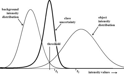
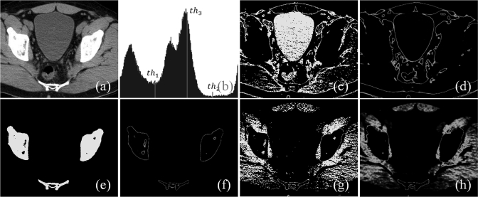
In this section, we define class uncertainty based on priors and describe its relation with the gradient feature derived from spatial distribution of image intensity values. Let us consider a simple example of Fig. 1 containing an object and a background region with their prior intensity distributions. Image points with intensity value of either or will be classified as object points; however, the class uncertainty values for these two cases are significantly different. Specifically, points with intensity value should possess significantly high class uncertainty as compared to those points with intensity value . The relation between class uncertainty and image features may be better understood with the help of a real image. Figure 2 illustrates the idea on an image slice from a lower abdominal CT data set of a patient. The image depicts several regions including fat/skin, bladder, muscles and bone which are partially separable using intensity thresholding. Three threshold values are manually picked on the intensity histogram [Fig. 2b] of the CT image slice [Fig. 2a] among which two thresholds, namely, and separate meaningful tissue regions [Figs. 2c, 2e] while is intentionally selected as a bad threshold not representing any meaningful tissue region [Fig. 2g]. It may be noted that class uncertainty images corresponding to thresholds and trace respective tissue boundaries [Figs. 2d, 2f] while that for the wrong threshold does not and the uncertainty image shows high values all over the homogeneous region [Fig. 2h].
Figure 1.
An illustration of the relationship among prior class distributions and class uncertainty for a two-class problem. It may be noted that class uncertainty is maximum around the threshold selected under minimum error criterion. Image points with intensity values of either or are classified as object points. However, the class uncertainty associated with points having intensity is significantly higher than that for points with intensity .
Figure 2.
An illustration of the relationship between class uncertainty and tissue interfaces under different conditions of thresholding. (a) An image slice from a CT data of a patient’s lower abdomen. (b) Image intensity histogram for (a) with three thresholds marked as , , and . The first two thresholds are manually selected to segment proper tissue regions while the third one is intentionally picked as a bad threshold. (c,d) Thresholded tissue regions and class uncertainty image for the threshold . (e,f), (g,h) Same as (c,d) but for thresholds and , respectively. Note that class uncertainty images in (d) and (f) depict respective tissue boundaries while the same in (h) fails to indicate any tissue interface and spills out into the entire soft tissue region.
An important observation in the above example is that when proper thresholds are selected to separate different tissue regions, corresponding class uncertainty maps depict interfaces among respective regions. On the other hand, when a visually incorrect threshold is selected, the class uncertainty map no longer describes a region boundary. This correlation between the two independently defined features lays the theoretical foundation for our method which is stated in the following postulate.51
Postulate 1. In an image with fuzzy boundaries, under optimum partitioning of object classes, intensities with high class uncertainty appear around object boundaries.
Although it is difficult to prove or disprove the postulate because of its nature, its validity may be justified on real-life images as demonstrated in Fig. 2 and the other experimental results presented in this paper.
Here, we formulate the mathematical expression for class uncertainty from priors using Bayes’ rule6 and Shannon and Weaver’s entropy equation.52 An image may be described by its intensity function where Z denotes the set of integers and R denotes the set of real numbers. In most acquired digital images, intensity values are readily available at points with integral co-ordinates which are called a “pixel” in two-dimension (2D) and a “voxel” in three-dimension (3D); we denote the set of all pixels or voxels in an image as C. In this paper, we use “point” to refer to a pixel or a voxel and denote a point by a vector whose elements denote coordinates along different axes. Let and represent the hypothetical true object and background regions, respectively, in an image. Let denote the prior probability distribution for object/background region defined as follows:
| (1) |
where P represents “probability,” p denotes an image point, and g is a given intensity value. Let θ denote the density for object points so that is the density for background points. Therefore, the probability of any point p having intensity value g, denoted by , may be expressed as follows:
| (2) |
Using the above priors, the posterior probabilities are defined by Bayes’ rule, i.e.,
| (3) |
Finally, the class uncertainty measure51 at a point p with intensity value g is defined as the entropy of the above two posterior probabilities which is defined by the Shannon and Weaver’s entropy equation52 as follows:
| (4) |
Here, the idea is to model the prior probability distributions and and the density parameter θ as a function of the selected threshold t and the gradient parameter σ. Thus, the class uncertainty map of an image varies as a function of threshold t and gradient parameter σ; we use to denote the threshold and gradient-dependent class uncertainty function. The methods for computing prior probability distributions and and the density parameter θ for a given pair of threshold and gradient values are described in Sec. 3.
Previously, Saha and Udupa51 showed the use of class uncertainty and Postulate 1 for optimum threshold selection and later Saha et al.53 demonstrated its use for improving the performance of a Snake-based segmentation algorithm. However, a major limitation of Saha and Udupa’s method is that they used an ad hoc approach for computing a normalized measure for gradients which is essential to couple it with class uncertainty using Postulate 1. Here, we overcome this problem and present the theory to simultaneously optimize both threshold and gradient parameters for individual tissue interfaces. In the following, we formulate an energy function that is used for threshold and gradient optimization.
Energy surface and threshold/gradient optimization
As mentioned earlier, the central theme of this paper is to couple the information embedded in the spatial arrangement of different object regions in an image with the class uncertainty measure derived using a probabilistic model and the theory of chaos. Specifically, we use Postulate 1 to combine the image-derived gradient feature with the prior based class uncertainty map to develop an energy function toward solving the problem of simultaneous threshold and gradient optimization for unknown number of object interfaces. It is not difficult to find out from Eq. 4 that the class uncertainty measure always lies in the normalized scale of [0, 1]. On the other hand, image gradient is measured in the image intensity scale. Therefore, a meaningful formulation of the energy function using Postulate 1 entails a normalized measure for image gradient values. To overcome this issue, a gradient parameter σ is introduced which needs to be optimized and, quite possibly, the parameter may not remain constant for different tissue interfaces. Many models may be adopted to normalize the gradient measure; here a Gaussian model is used to compute a normalized measure of intensity gradients using the control parameter σ as follows:
| (5) |
where ∇ is an intensity gradient operator and is a normalized gradient parameter. Using these two normalized measures of class uncertainty and image gradient, the energy function E is formulated as follows:
| (6) |
Following the above equation, each point p contributes large energy if it falls in any of the following two categories—(1) class uncertainty is high and gradient is low or (2) class uncertainty is low and gradient is high. It may be noted that each of these two situations is a contradiction to Postulate 1. To some extent, the energy function E is formulated as an aggregate measure of contradictions to Postulate 1 over the entire image. On the other hand, if a pixel p has both high class uncertainty and high gradient or low value for both measures, it’s in agreement with Postulate 1 and only contributes a small amount of energy. It may be noted that, under any of these two conditions, each of the two components on the right hand side of Eq. 6 takes a small value (close to “0”) due to the multiplication between a high (close to “1”) and a low (close to “0”) value and therefore the sum of the two components is always a small value. In Sec. 3 , we describe details related to a new method based on the theoretical foundation laid in this section. Also, in the same section, we describe experimental plans evaluating the method.
METHODS AND EXPERIMENTAL PLANS
In Sec. 2 , we have formulated an energy function E that captures the correlation between image gradient and class uncertainty as guided by Postulate 1. Specifically, the energy function is formulated as an aggregate measures of contradictions to Postulate 1 by all points in an image and is expressed as a function of threshold and gradient parameters t and σ, respectively. Thus, the energy function E essentially forms an energy surface over the parametric space of t and σ and an optimum choice of threshold and gradient parameters representing an object interface may be found by identifying a meaningful depression on the energy surface. Following the theoretical formulations of Sec. 2, we need to define the following steps to compute the energy function:
-
1.
Computation of the original and normalized gradient maps ∇ and , respectively.
-
2.
Computation of prior intensity probability distributions and and the density parameter θ for given values of threshold and gradient parameters t and σ.
Finally, it is necessary to identify the optimum values of t and σ on the energy surface E. In the following paragraphs, we describe these steps in details.
The initial gradient map ∇ is computed in image intensity scale using a derivative of Gaussian (DoG) type edge operator6 to reduce the effects of noise. To accomplish it, first, a blurring operation is applied on the original image using a Gaussian smoothing kernel6 currently available under ITK application libraries.54 The shape of the smoothing kernel (i.e., sharp or wide) may be controlled using a standard deviation parameter ; in this paper, a constant value of two points is used for the kernel parameter . Let denote the intensity function for the blurred image. The gradient map in the intensity scale is computed from the blurred image as follows:
| (7) |
and
| (8) |
where , , and are unit vectors along the x-, y-, and z-coordinate axes, respectively. The computation of the intensity gradient map immediately generalizes to any higher dimension. Finally, the normalized gradient map is computed from the intensity gradient map using Eq. 5 for a given value σ of the gradient parameter.
In order to make the class uncertainty map more consistent with the gradient map computed using a DoG operator, the blurred image is used for class uncertainty computation. The blurring operation also reduces the effects of noise and enhances the statistics of class uncertainty maps, especially, for sharp interfaces. It may be noted that, once the optimum thresholds and gradients are determined, they are applied on the original image; thus, the blurring used during the process of threshold and gradient optimization does not incur any structural loss or blurring in final thresholding results.
For a given pair of values of threshold and gradient parameters t and σ, prior object and background intensity distributions and are modeled using the following equations:
| (9) |
and
| (10) |
Here, and are used as reference object and background intensities because they dedicate a intensity band (covering ∼99.7% of population) for the interface between the object and background regions. In Eq. 6, the original intensity function f is replaced by the blurred image intensity function for computing class uncertainty values. Finally, the density function θ is computed as the ratio of the number of points in each of the two thresholded regions.
Optimization of threshold and gradient parameters
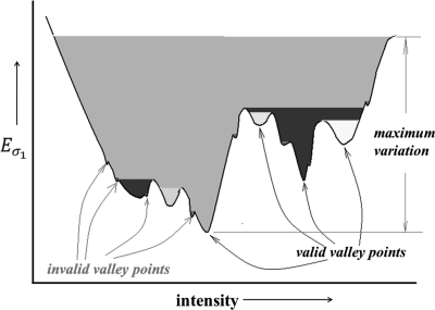
In this section, we describe the optimization technique for threshold and gradient parameters t and σ over the energy surface E described in Sec. 2 . Following that the search-space is only two-dimensional over a limited range of values for t and σ, we adopt an exhaustive search technique. Therefore, the most critical factor here is to define the geometry of optimum locations on the energy surface. For the threshold parameter t, the entire intensity range is used for searching optimum locations. On the other hand, search-space for the gradient parameter σ is limited to ; we stay away from the extreme values of σ to reduce computation burden and also, to avoid computational instability. We determine two types of optimum locations on the energy surface—a type I optimum location forms a meaningful or valid pit on the energy surface E while a type II optimum location forms a meaningful valley on E. Let denote energy function for a given value of the gradient parameter and thus, only the threshold parameter is varied. Therefore, forms an energy curve for the gradient parameter value . A local minimum on the energy surface E is referred to as a pit while a local minimum on an energy line is referred to as a valley point. Depending upon the resolution of the search-space, both E and may contain a large number of noisy local minima. Here, we use the idea of intrinsic basin, an idea similar to catchment basins used in watershed segmentation methods,55, 56 to distinguish between noisy and meaningful local minima. Let denote the parameter values at a pit, i.e., a local minimum on the energy surface E. The intrinsic basin of , denoted by , is the set of all locations such that there exists a path from to with all points on the path having energy values greater than or equal to . Essentially, corresponds to the region on E that can be flooded by pouring water from top at without water leaking to a location with energy value less than . An intrinsic basin for a valley point , i.e., a local minimum on the energy curve is defined similarly. The idea of intrinsic basin on an energy line is illustrated in Fig. 3. The black line in Fig. 3 denotes the energy line over the entire intensity range and each local minimum on the line represents a valley point. Different colors are used to indicate different intrinsic basins; however, one intrinsic basin may include multiple colors. The depth of a basin is defined as the height of its topmost layer with respect to its bottom. A pit (or, a valley point) is considered as a valid pit (respectively, a valid valley point) if the height of its intrinsic basin covers at least 3% of the maximum variation in the energy surface E (respectively, the energy line ). The maximum variation for the energy curve , illustrated in Fig. 3, is the depth of the grey basin. Depths of basins marked as invalid valley points are less than 3% of the maximum variation and thus fail to quality as valid valleys; all other basins in Fig. 3 qualify as valid valleys. The choice of the parameter value of 3% for validity check was selected as it was experimentally observed that the height of intrinsic basins for noisy points were small and was always less than 1%. Therefore, the parameter value of 3% ensures exclusion of all noisy points.
Figure 3.
An illustration of intrinsic basins on an energy line . Different colors are used to indicate different intrinsic basins; however, one intrinsic basin may include multiple colors. All invalid valley points are marked in a different color than valid valley points.
In our experiments, both energy surfaces and curves are mostly found to be smooth functions except for tiny fluctuations, especially, over flat regions. The primary objective of adding a validity constraint on pits and valley points using intrinsic basins is to avoid such small fluctuations while capturing all meaningful local minima. Each valid pit is considered as a type I optimum location for threshold and gradient parameters. A meaningful valley is defined as an eight-connected path57, 58 of valid valley points for contiguous values of the gradient parameter. Finally, a type II optimum point is defined at the center of a meaningful valley containing no pit or type I optimum location. Thus the search step for optimization of threshold and gradient parameters may be summarized as follows:
Algorithm.
. Search_Local_Minima_on_Energy_Surface.
| Input: |
| : energy surface where t and σ are threshold and gradient parameters, respectively |
| Output: |
| Types I and II optimum locations for threshold and gradient parameters |
| Begin: |
| for all values of the threshold parameter tdo |
| for all values of gradient parameter σdo |
| if is a valid pit |
| select as a type I optimum location for threshold and gradient parameters |
| ift is a valid valley point on |
| find the eight-connected path π of valid valley points containing |
| ifπ contains no valid pit or type I optimum location |
| select a type II optimum location on π |
| end |
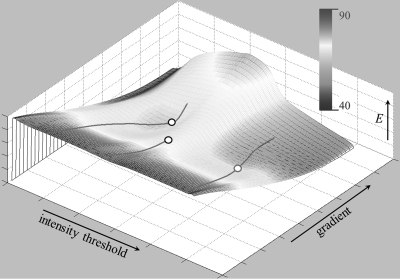
An example of the energy surface/function and detected optimal locations are illustrated in Fig. 4. For the current example, three valley lines were identified on the energy surface among which two were associated with pits or type I optimal locations while one valley had no pit on it. For the valley with no pit, a type II optimal location was detected following the algorithm described in the above.
Figure 4.
An illustration of different types of optimum locations on an energy surface/function. The energy function is rendered using a 3D matlab display function with color indicating the energy value. Here, valley lines are shown with Types I (pit) and II optimum locations on the energy surface are denoted by hollow circles of different colors.
Experimental plans
Here, we describe our experimental plans to examine the effectiveness of the proposed thresholding algorithm and to compare its performance with Otsu’s method21 and several other popular thresholding methods.33, 35, 51 Although, the thresholding method by Otsu was proposed three decades ago, it has become quite popular because of its classical theoretical foundation. Recently, the method has been implemented within the ITK library54 and has been used in several medical imaging8, 9, 10, 11, 12, 13 and other applications.59, 60, 61, 62 Essentially, the method is based on minimization of the class density weighted within-class variance which is also equivalent to maximization of between-class variance. A limitation of Otsu’s method is that it requires that the number of tissue regions must be specified. In our experimental setup we used Otsu’s method with the correct number of tissue regions specified by users. On the other hand, for the proposed method, this number is detected automatically by the algorithm. Also, we have compared the performance of the new method with the minimum error (ME) (Ref. 33) and maximum segmented image information (MSII) (Ref. 35) thresholding algorithms along with our previously published minimization of homogeneity- and uncertainty-based energy (MHUE) thresholding algorithm.51 The principle of ME thresholding algorithm is to find the threshold that gives minimum classification error defined as follows. For a given threshold, an image is partitioned into two regions and the normal distribution of intensity values within each partition is determined. The classification error is determined as the average fraction of the normal intensity distribution of one partition falling inside the intensity range of the other. The principle of the MSII thresholding algorithm is based on maximization of segmented image information defined as the difference between initial scene uncertainty, computed from the original image, and residual uncertainty computed from the thresholded image. In the MHUE (Ref. 51) thresholding algorithm, the class uncertainty theory is combined with a rank-based normalized measure of region homogeneity to formulate the criterion of threshold optimization.
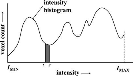
Experiments were designed to evaluate both accuracy and reproducibility of the new method and to compare with the other methods. The accuracy of a method was computed by comparing its results with manual thresholding except for phantom data where truths were known. Reproducibility of a method was computed using repeat scan multidetector computed tomography (CT) data of cadaveric ankle specimens. In order to reduce subjectivity artifacts by individuals for accuracy analyses on clinical data, the mean of threshold values selected by three independent users for a given interface was used as truth. Toward defining an error measure between a computer-selected threshold s and a true threshold t, an important observation was made that pixel/voxel density is nonuniform over the intensity range. Therefore, a straight-forward difference between s and t may not be a good choice for error measure. Let , where is the set of positive integers, denote the image intensity histogram function. The value of denotes the pixel/voxel density at the intensity value i. We use the following error function which essentially represents the pixel/voxel density weighted distance between s and t in the normalized scale of [0,1] defined as follows:
| (11) |
where represents the intensity histogram of the test image. The idea of the above error measure is graphically illustrated in Fig. 5. When there are multiple true thresholds , , , … and computed thresholds , , , … for different object regions, for each true threshold the closest computed threshold is used for estimating the error. In the following, we describe different image data sets used in our experiments.
Figure 5.
A graphical illustration of the error measure between a selected threshold s and the true threshold t. Essentially, it computes the pixel/voxel density weighted distance (the area of the grey region) between the two thresholds and normalize by image size, i.e., the total area under the histogram.
CT image of cadaveric ankle specimens: Four cadaveric ankle specimens were scanned in a Siemens Sensation 64 Multislice CT scanner at 120 kVp and 140 mAs and a pitch of 0.8 to adequately visualize the bony structures. After scanning in a helical mode at a slice thickness of 0.6 mm and collimation of 12 × 0.6 mm, the image was reconstructed at 0.3 mm slice thickness with a normal cone beam method utilizing a very sharp kernel of U75u to achieve high image resolution. Image parameters for these scans were as follow: matrix size = 512 × 512 pixels; number of slices = 334–336; pixel size = 152 μm. Each ankle specimen was scanned three times after repositioning on the table. This CT data set was used for both accuracy and reproducibility analysis.
Simulated brain MRI: T1-weighted MR phantom images at different levels of noise, intensity nonuniformity and slice thickness were downloaded from the online facility supported by Brainweb.63 Specifically, six MR images at 0%, 1%, 3%, 5%, 7%, and 9% noise levels provided by the above referred online site were used for our experiments. Seven MR images at 1%, 2%, 5%, 10%, 15%, 20%, and 25% intensity nonuniformity were generated from the original image and the degraded image at 20% intensity nonuniformity provided at the website. Image parameters for all images at varying noise and intensity nonuniformity levels are as follows: matrix size = 181 × 217 pixels; number of slice = 181; isotropic voxel size = 1 mm. Also, another set of five images at varying slice thickness of 1, 3, 5, 7, and 9 mm was used to examine the performance of the method under varying resolution.
RESULTS AND DISCUSSION
Qualitative results
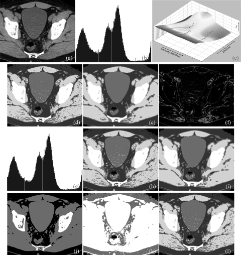
Results of application of the method on 2D and 3D CT images are presented in Figs. 678. Figure 6a shows a 2D image slice from a lower abdominal CT image of a patient containing different tissue regions/organs, namely, bone, muscle, bladder, fat/skin and air that are visually detectable. The intensity value for the air space in this image is exactly “0” and therefore, the region with zero intensity value was excluded from analysis. The automatic threshold and gradient selection method was applied over regions with nonzero intensity values and three thresholds were detected [Fig. 6b] segmenting the image into four regions [Fig. 6d] corresponding to fat/skin, bladder, muscles and bone. The energy surface and detected optimal threshold and gradient parameter locations are illustrated in Fig. 6c. In Fig. 6d, different thresholded regions are marked with different colors. It may be noted that around each muscle region, there is a thin layer of missclassified bladder region caused by partial voluming effect. Also, noisy speckles are visible on thresholded regions in Fig. 6d which disappear on a smooth image shown in Fig. 6e. The class uncertainty image at different thresholds is presented in Fig. 6f where different colors are used to describe interfaces between respective tissue regions. It is interesting to note how the class uncertainty image depicts different object boundaries. The method has been found stable despite noise and low contrast between bladder and muscles. Also, Otsu’s thresholding algorithm was applied to this image (over regions with nonzero intensity values) and the results are presented in Figs. 6g–6i. For Otsu’s method, the number of tissue regions was provided externally. Beside this limitation of Otsu’s method, results of the two methods are visually similar for this example. Results of application of MSII, ME, and MHUE algorithms are shown in Figs 6j–6l, respectively; while MHUE has produced visually satisfactory results, ME and MSII have clearly failed to detect different tissue regions.
Figure 6.
Results of application of different thresholding methods on a CT image slice of lower abdomen. (a) Original CT image slice. (b) Optimum thresholds (red lines) derived by the new method. (c) The energy surface with valley lines and optimum threshold and gradient parameters (hollow circles). (d) Thresholded regions in different colors as applied to the original image. (e) Same as (d) but applied to a smoothed image. (f) Object class uncertainty maps at different optimum thresholds. Note that the class uncertainty image highlights different tissue interface at different optimum thresholds. (g,h,i) Same as (b,d,e), respectively, but for Otsu’s method. (j,k,l) Results of thresholding as obtained by the MSII, ME, MHUE algorithms, respectively. One of the merits of the proposed method is that by incorporating spatial information, the new method succeeds in dealing with all three examples of Figs. 678; however, Otsu’s method succeeds in Fig. 6 but clearly fails in Fig. 8.
Figure 7.
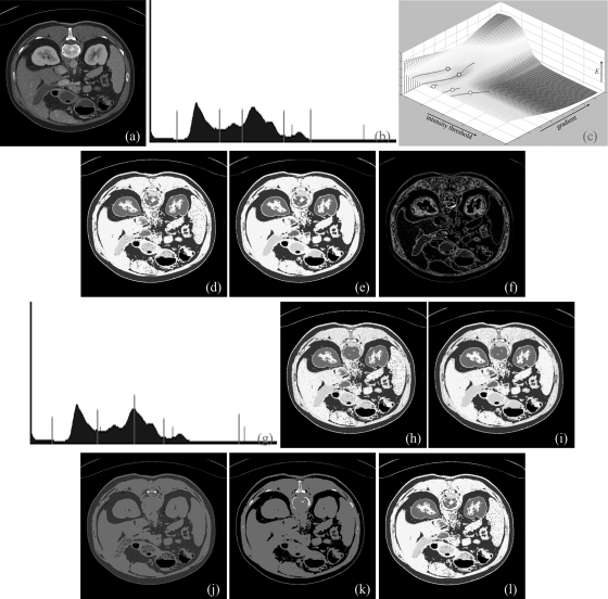
Same as Fig. 6, but for a CT image slice of upper abdomen.
Figure 8.
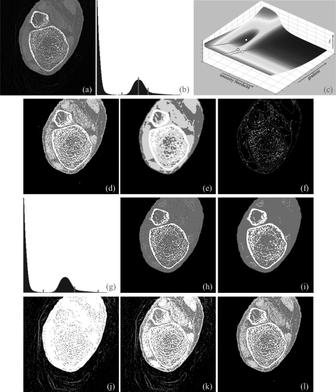
Same as Fig. 6, but for a 3D CT image of a cadaveric ankle specimen.
Results of application of the method on another image are illustrated in Fig. 7. Figure 7a shows a 2D image slice from upper abdominal CT image of a patient containing different regions with visibly distinct intensity values. Our method was applied on this image slice and five different optimal thresholds were identified [Figs. 7b, 7c]. Six thresholded regions, including air, are depicted in Figs. 7d, 7e using a separate color for each thresholded region. The class uncertainty maps for different thresholds are displayed in Fig. 7f using different colors for different thresholds which indicates different tissue interfaces. Results of application of Otsu’s method are presented in Figs. 7g–7i. As visually appear in Fig. 7g, Otsu’s method has under thresholded the region representing muscle, spleen and liver while it has over thresholded the bone region. Results of application of MSII, ME, and MHUE algorithms are shown in Figs. 7j–7l, respectively; while MHUE has produced visually satisfactory results similar to the new algorithm, ME and MSII have clearly failed to detect different tissue regions.
Accuracy analysis
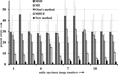
As described in Sec. 3B, the following image data sets were used to examine the accuracy of the new method as compared to Otsu’s method and three other popular thresholding methods—(1) three repeat CT scans of four cadaveric ankle specimens (altogether, twelve images), (2) six MR phantom images from the brain web data set with noise level varying over 0%–9%, (3) seven MR phantom images from the same dataset with intensity nonuniformity levels varying over 1%–25%, and (4) five MR phantom images from the same data set with slice thickness varying over 1–9 mm. All 12 ankle images were used for this experiment and results of application of the new method and those of other methods on one ankle specimen are illustrated in Fig. 8. The new method successfully detected three thresholds producing visually satisfactory segmentation of four regions, namely, background, fat/skin, muscle, and bone. Salt and pepper noise, especially, over thresholded regions for fat/skin and muscle [Fig. 8d] was primarily caused by low contrast-to-noise-ratio between the two regions which disappeared after applying a simple smoothing filter [Fig. 8e]. More interesting, the amount of noise on each of the two regions is more or less similar indicating that the method selected the threshold nearly at the middle between mean intensities for the two regions. In Fig. 8b, the second threshold on the intensity histogram of the 3D image represents the threshold for the interface between the two regions which is located near the second pick of the histogram. Just by looking at the histogram it is almost impossible to select this threshold. On the other hand, the two regions and therefore the interface threshold is clearly visible in the image which allowed our algorithm to automatically detect the threshold. As shown in Fig. 8c, each of the first two thresholds led to pits (type I optimum locations) while the third threshold produced only a valley (type II optimum location). The class uncertainty image at different thresholds successfully depicts different interfaces with different colors. Otsu’s method has failed to produce visually satisfactory results for this example. Also, ME and MSII thresholding methods have failed to find thresholds for all three tissue interfaces in these images significantly increasing error measures. For this specific specimen, the MHUE has produced almost similar results [Fig. 8l] as produced by the new algorithm. For quantitative accuracy analysis, gold standard threshold for each interface for each image was determined as the average of the thresholds selected using a graphical user interface by three independent users to reduce the effect of interuser subjectivity errors. For a given CT image and a specific tissue interface, the threshold error by a method was determined from the true threshold and the closest computed threshold according to the error definition presented in Sec. 3B. Finally, for a given image, the threshold error was computed as the sum of errors over all interfaces. Images threshold errors for twelve images by the five methods are illustrated in Fig. 9 using bar diagram. Also, the standard deviation of threshold errors for different interfaces in an image is indicated in the figure. The new method has clearly outperformed the ME and MSII thresholding methods. Average image threshold errors by Otsu’s and MHUE methods are 20.78% and 8.57%, respectively, while that by the new method is only 2.75% indicating seven- and three-fold error reduction as compared to Otsu’s and MHUE methods, respectively. Also, the standard deviation of threshold errors for different tissue interfaces by the new method is relatively small for all images indicating the consistency of our method in selecting the threshold for different tissue interfaces. As described in Sec. 4B, average image threshold error was measured by adding errors from all interfaces. For example, each ankle CT data used here has three tissue interfaces; therefore, the average interface threshold error by our method should be 0.92% computed by dividing the total image threshold error of 2.75% by three. We performed a paired t-test of threshold errors by the new, the Otsu’s and the MHUE methods using the error values for all three interfaces in all images. The average threshold errors for an interface by Otsu’s, MHUE and the new methods are 6.93%, 2.86%, and 0.92%, respectively, and the null hypothesis was rejected with p-value < 0.001 for comparisons between the new and either of Otsu’s or MHUE methods.
Figure 9.
Results of quantitative analyses of image threshold errors by different methods. For each ankle CT image, indicated by a number between one and twelve on the horizontal axis, height of the bar indicates the percent image threshold error. The line one each bar denotes the standard deviation (in percentage scale) of threshold errors for different interfaces in an image.
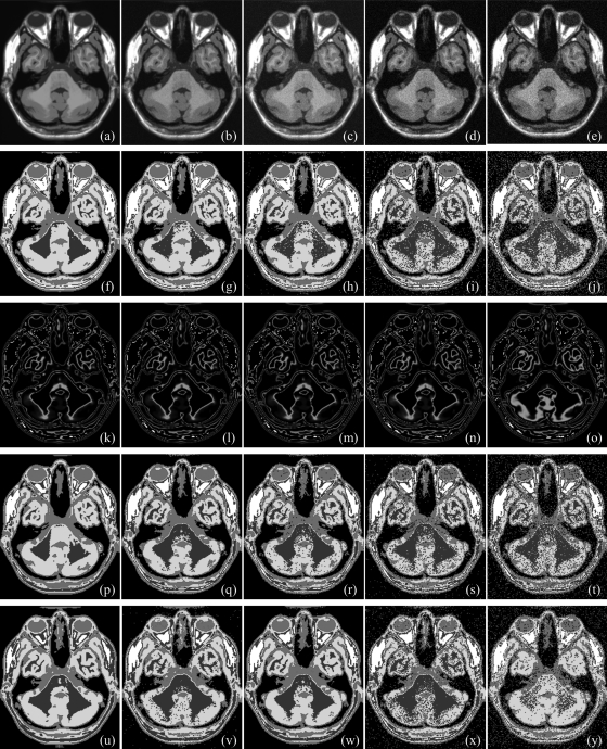
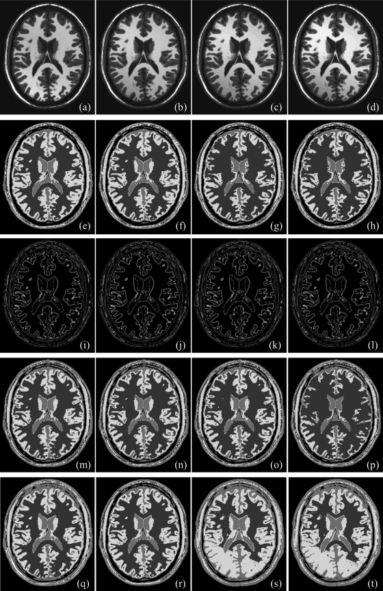
Results of application of the new method and those of Otsu’s method on the MR brain phantom image at varying noise levels are illustrated in Fig. 10. Figures 10a–10e illustrate matching image slices from phantom data at 0%, 3%, 5%, 7%, and 9% noise. For all 3D images at different noise levels, both new and Otsu’s methods detected four thresholds producing visually satisfactory results; see Figs. 10f–10j and Figs. 10p–10t. Class uncertainty images at different noise levels for different thresholds using our method are presented in Figs. 10k–10o; similar to the other examples, class uncertainty images at different thresholds nicely represent different interfaces. Results of thresholding using the MHUE algorithm are presented in Figs. 10u–10y; although MHUE produced similar results to the new algorithm at low noise, the results at high noise [Fig. 10y] is visually less satisfactory. Figure 11 illustrates same results at different slice location from 3D images. Results of application of the new, Otsu’s and the MHUE thresholding methods on MR brain phantom images with varying intensity nonuniformity are qualitatively illustrated in Fig. 12. Figures 12a–12d shows the matching slice from phantom images at 10%, 15%, 20%, and 25% intensity nonuniformity. As observed in Figs. 12e–12h, 12m–12p, both the new and Otsu’s methods are found quite robust under moderate intensity nonuniformity. However, a thresholding method may fail at higher levels of intensity nonuniformity where significant overlap takes place between intensity distributions of two tissue types at different spatial locations. The MHUE algorithm have failed to produce visually satisfactory results (Figs. 12s, 12t] at 20% and 25% intensity nonuniformity.
Figure 10.
Results of thresholding on MR brain phantom images at different noise levels: 0% (a), 3% (b), 5% (c), 7% (d), and 9% (e). (f–j) Results of thresholding by the new method for (a–e), respectively, at different noise levels. (k–o) Class uncertainty images at optimum thresholds of (f–j), respectively. (p–y) Same as (f–j) but for Otsu’s (p–t) and the MHUE (u–y) methods, respectively.
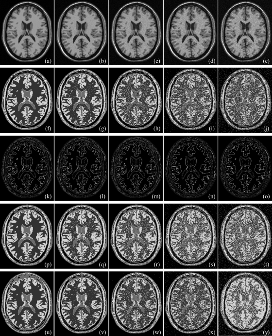
Figure 11.
Same as Fig. 10 but at a different slice location.
Figure 12.
Same as Fig. 10 but at different nonuniformity levels: 10% (a), 15% (b), 20% (c), and 25% (d) intensity nonuniformity. Here, a display-intensity window different from Figs. 1011 was used to illustrate the intensity nonuniformity.
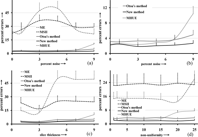
Qualitative results on Brainweb MR phantom images at different levels of noise and intensity nonuniformity illustrated in Figs. 101112 do not lead to a decisive conclusion about the performance of the new, Otsu’s and MHUE methods. For this reason, we performed a quantitative comparison among the results by different methods in the same way we did for the example of ankle images. Errors of different image thresholding methods at different levels of noise are presented in Fig. 13a as functions of noise; results of comparison with Otsu’s and MHUE methods are magnified in Fig. 13b. Figures 13a, 13b shows that the new method clearly outperforms (smaller errors) ME and MSII methods and also, generates less error than Otsu’s methods at every level of noise. As compared to the MHUE method, the improvement by the new method is enhanced at higher noise levels. Similar to the example of ankle image, we performed a paired t-test of threshold errors by the new and Otsu’s methods using the error values for all four interfaces in images with varying noise. The average threshold errors for an interface by the new, Otsu’s and MHUE methods are 0.56%, 0.88% and 1.02%, respectively, and the null hypothesis was rejected with p-value = 0.01 for comparison between the new and Otsu’s methods and the p-value observed was 0.07 for comparison between the new and MHUE methods. For the experiment at varying thickness levels, results of quantitative comparison among the results from the five methods in terms of image threshold errors are presented in Fig. 13c as a function of slice thickness. The results of paired t-test between our method and Otsu’s method are as follows: average threshold errors for an interface by the new, Otsu’s, and MHUE methods are 0.65%, 1.05%, and 1.13%, respectively, and the null hypothesis was rejected with p-value < 0.001 for comparison between the new and Otsu’s methods and the p-value observed was equal to 0.21 for comparison between the new and MHUE methods. The experimental results of Fig. 13d at different levels of intensity nonuniformity confirm the same trend observed in Figs. 13a–13c at varying noise and slice thickness. The results of paired t-test between our method and Otsu’s method at different levels of intensity nonuniformity are as follows: average threshold errors for an interface by the new, Otsu’s, and MHUE methods are 0.64%, 1.13%, and 0.97%, respectively, and the null hypothesis was rejected with p-value < 0.001 for comparison between the new and Otsu’s methods and the p-value observed was 0.06 for comparison between the new and MHUE methods. In general, the performance of the previously published MHUE thresholding algorithm was comparable to that of the new algorithm under small imaging artifacts with noise, intensity nonuniformity and slice thickness. However, the performance of the MHUE algorithm was degraded as levels of those artifacts were raised. This inconsistency in performance of the MHUE algorithm has reduced the statistical significance in the results of paired t-test analyses.
Figure 13.
Results of quantitative comparison on MR brain phantom images at varying levels of noise, slice thickness and intensity nonuniformity. (a) Errors for different image thresholding algorithms as functions of noise level. (b) Same as (a) but without MSII and ME. (c, d) Same as (a) but as functions of slice thickness (c) and intensity nonuniformity (d).
Reproducibility analysis
As described in Sec. 3B, three repeat CT scan data of four cadaveric specimens were used for reproducibility analysis. We performed two reproducibility analyses as follows:
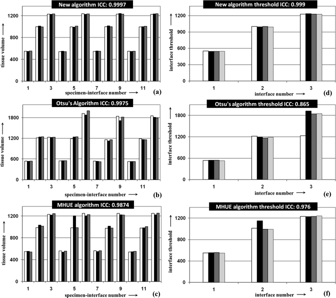
Experiment 1: For this experiment, repeat CT scans were used to examine the reproducibility of threshold values for different interfaces and specimens. From every CT image, we extracted three data values, each representing the threshold value for one of the three tissue interfaces (see Sec. 4B). Thus, altogether there were twelve events each representing the threshold for a specific interface in a given specimen [Figs. 14a–14c]. The threshold value computed from each repeat CT scan was considered as a repeat observation of the event; thus, there were three repeat observations. Results of this experiment are presented in Figs. 14a–14c showing that high repeat scan reproducibility for all three methods except that the MHUE algorithm has underperformed for one specimen (specimen-interface number 5) where it missed the threshold for one tissue interface.
Figure 14.
Results of reproducibility analysis and intraclass coefficient (ICC) of threshold values in repeat CT scans. (a) ICC for threshold values of different tissue interfaces of four specimens in three repeat scans using the new method. (b) Same as (a) but for Otsu’s method. (c,d) Same as (a,b) but for ICC value of thresholds for matching interfaces in different specimens using the first CT scan.
Experiment 2: The purpose of this experiment was to examine whether a method reproduce the same threshold for a specific tissue interface in different specimens. The argument behind this experiment is that, in CT images, intensity values for different tissues are highly reproducible64 and therefore, different methods should produce similar thresholds for a specific interface in different specimens. For this experiment, we used the data from first CT scan for each of the four specimens. Here, threshold of a given tissue interface is considered as an event leading to three events for three interfaces. On the other hand, the threshold values of the specific tissue interface computed from different specimens are treated as repeat observations leading to four observations for each event. Results of this experiment for the new, Otsu’s and MHUE methods are presented in Figs. 14d–14f. ICC values for the three methods under this experiment are 0.999, 0.865, and 0.976, respectively. Similar results were found using images from other two scans.
Results of above two experiments show that all three methods successfully reproduce a threshold in repeat scans for a specific interface in a given specimen. However, Otsu’s method has failed to guarantee high reproducibility of the threshold for a specific interface in different ankle specimens which is expected to be similar in CT images. The MHUE method is less robust in detecting all different tissue interfaces in an images resulting reduced ICC values in both reproducibility experiments. The new method has shown high reproducibility under both experiments. In repeat CT scans of a given specimen, histograms are similar; on the other hand for different specimens, there were significant variations in histograms due to differences in tissue proportions. It explains the behavior of Otsu’s method in above two experiments.
Conclusion and discussion
In this paper, we have presented a new method for simultaneously computing optimum values for thresholds and gradient parameters for different object interfaces. The method has been applied on several medical image data sets. For every example presented here, the new method has successfully determined the number of object/tissue regions in the image and also, detected visually satisfactory thresholds for different tissue interfaces even when some of the thresholds are almost impossible to locate in their histograms. Although, the method provides the optimum gradient parameter for each interface in an image, the accuracy and reproducibility of this parameter has not been examined in this paper. Accuracy and reproducibility of the new thresholding method have been evaluated using both clinical CT images and MRI brain phantoms data sets. The performance of the method has been compared with two types of methods—(1) methods with automatic detection of the number of object regions (ME, MSII, MHUE) and (2) methods with predefined number of object regions (Otsu). Results of comparative experiments have shown that the new significantly outperform the two methods (ME and MSII) under the first category. Results of comparison with Otsu’s method has shown that, given the predefined number of object regions, Otsu’s method produce visually similar results to our method where the thresholds are visible (e.g., a local plateau) on the histogram. However, Otsu’s method being a purely histogram-based algorithm; it may fail to properly select a threshold when it is located near a local top on the histogram (Fig. 8). On the other hand, our method effectively utilizes spatial information by combining image gradient with class uncertainty. Therefore, although, the information on the histogram is not good enough to select the right threshold, the new method fills the gap by using spatial information. Further, one major advantage of the current method over Ostu’s method is that the new method does not require any predefined number of object region in an image which itself is a significant improvement. Even for the examples where Otsu’s method produce results visually similar to the new method, quantitative analyses of accuracy and reproducibility have shown that the new method is superior to Otsu’s method. As compared to the MHUE algorithm, the improvement in performance of the new algorithm is enhanced as higher levels of imaging artifacts by noise, intensity nonuniformity and resolution. Also, the MHUE algorithm was found less robust in detecting thresholds for all tissue interfaces.
All methods were implemented on a Desktop PC with Intel(R) Xeon(R) CPU at 2.27GHz running under a Linux operating system. For a 3D Brainweb image of size 181 × 217 × 181 (Fig. 10), the ME and MSII methods take approximately 1 s to complete the task. Time complexity for Otsu’s method depends on the number of object regions in an image. It takes approximately 1 s for three objects, 3 s for four objects, and 40 s for five objects and it increases exponentially with the number of objects in an image. Running time for the MHUE algorithm and our new method are both independent of the number of objects regions but increases linearly with image size. For the 3D Brainweb image (Fig. 10), the running time is around 30 s for MHUE, while the computation time of our method approximately 41 s. Overall, the new algorithm improves the accuracy and robustness of image thresholding without any prior knowledge of the number of object regions with some increased computational costs.
ACKNOWLEDGEMENT
This work was partially supported by the NIH Grant No. R01 AR054439.
References
- Rosenfeld A. and Kak A. C., Digital Picture Processing I and II (Academic, Inc., Orlando, FL, 1982), Vol. 1. [Google Scholar]
- Jain A. K., Fundamentals of Digital Image Processing (Prentice-Hall, Upper Saddle River, NJ, 1989). [Google Scholar]
- Udupa J. K. and Herman G. T., 3D Imaging in Medicine (CRC, Boca Raton, FL, 1991). [Google Scholar]
- Gonzalez R. C. and Woods R. E., Digital Image Processing (Addison-Wesley, Reading, MA, 1992). [Google Scholar]
- Bezdek James C. and Pal Sankar K., Fuzzy Models for Pattern Recognition: Methods That Search for Structures in Data (IEEE, New York, NY, 1992). [Google Scholar]
- Sonka M., Hlavac V., and Boyle R., Image Processing, Analysis, andMachine Vision, 3rd ed. (Thomson Engineering, Toronto, Canada, 2007). [Google Scholar]
- Bracewell R. N., Two-Dimensional imaging (Prentice-Hall, Inc., Englewood Cliffs, New Jersey, 1995). [Google Scholar]
- Filho E., Saijo Y., Tanaka A., Yambe T., Li S., and Yoshizawa M., “Automated calcification detection and quantification in intravascular ultrasound Images by adaptive thresholding,” Proceedings of World Congress on Medical Physics and Biomedical Engineering (COEX Seoul, Korea, 2007), pp. 1421–1425.
- Pappas I. P., Styner M., Malik P., Remonda L., and Caversaccio M., “Automatic method to assess local CT-MR imaging registration accuracyon images of the head,” AJNR Am. J. Neuroradiol. 26, 137–144 (2005). [PMC free article] [PubMed] [Google Scholar]
- Yang Y., Huang S., and Rao N., “An automatic hybrid method for retinal blood vessel extraction,” Int. J. Appl. Math. Comput. Sci., 18, 399–407 (2008). 10.2478/v10006-008-0036-5 [DOI] [Google Scholar]
- Asari K. V., Srikhanthan T., Kumar S., and Radhakrishnan D., “A pipelined architecture for image segmentation by adaptive progressive thresholding,” J. Microprocess. Microsyst. 23, 493–499 (1999). 10.1016/S0141-9331(99)00057-5 [DOI] [Google Scholar]
- Kumar S., Asari K. V., and Radhakrishnan D., “Real-time automatic extraction of luman region and boundary from endoscopic images,” Med. Biol. Eng. Comput. 37, 600–604 (1999). 10.1007/BF02513354 [DOI] [PubMed] [Google Scholar]
- Tian H., Srikanthan T., and Asari K. V., “Automatic segmentation algorithm for the extraction of lumen region and boundary for exdoscopic images,” Med. Biol. Eng. Comput. 39, 8–14 (2001). 10.1007/BF02345260 [DOI] [PubMed] [Google Scholar]
- Saha P. K., Udupa J. K., and Odhner D., “Scale-based fuzzy connected image segmentation: theory, algorithms, and validation,” Comput. Vis. Image Underst. 77, 145–174 (2000). 10.1006/cviu.1999.0813 [DOI] [Google Scholar]
- Zhuge Y., Udupa J. K., and Saha P. K., “Vectorial scale-based fuzzy connected image segmentation,” Comput. Vis. Image Underst. 101, 177–193 (2006). 10.1016/j.cviu.2005.07.009 [DOI] [Google Scholar]
- Sahoo P. K. and Soltani S., “A survey of thresholding techniques,” Comput. Vis. Graph. Image Process. 41, 233–260 (1988). 10.1016/0734-189X(88)90022-9 [DOI] [Google Scholar]
- Lee S. U., Chung S. Y., and Park R. H., “A comparative performance study of several global thresholding techniques for segmentation,” Comput. Vis. Graph. Image Process. 52, 171–190 (1990). 10.1016/0734-189X(90)90053-X [DOI] [Google Scholar]
- Glasbey C. A., “An analysis of histogram based thresholding algorithms,” CVGIP: Graph. Models Image Process. 55, pp. 532–537 (1993). 10.1006/cgip.1993.1040 [DOI] [Google Scholar]
- Prewitt J. and Mendelsohn M., “The analysis of cell images,” Ann. N. Y. Acad. Sci. 128, 1035–1053 (1966). 10.1111/j.1749-6632.1965.tb11715.x [DOI] [PubMed] [Google Scholar]
- Doyle W., “Operations useful for similarity-invariant pattern recognition,” J. ACM 9, 259–267 (1962). 10.1145/321119.321123 [DOI] [Google Scholar]
- Otsu N., “A threshold selection methods from grey-level histograms,” IEEE Trans. Pattern Anal. Mach. Intell. 9, 62–66 (1979). [Google Scholar]
- Ridler T. W. and Calvard S., “Picture thresholding using an iterative selection method,” IEEE Trans Syst. Man Cybern. 8, 630–632 (1978). 10.1109/TSMC.1978.4310039 [DOI] [Google Scholar]
- Trussell H. J., “Comments on ‘picture thresholding using an iterative selection method’,” IEEE Trans. Syst. Man Cybern. 9, 311 (1979). 10.1109/TSMC.1979.4310204 [DOI] [Google Scholar]
- Tsai W. H., “Moment-preserving thresholding: A new approach,” Comput. Vis. Graph. Image Process. 29, 377–393 (1985). 10.1016/0734-189X(85)90133-1 [DOI] [Google Scholar]
- Pun T., “A new method for gray level picture thresholding using the entropy of the histogram,” Signal Process. 2, 223–237 (1980). 10.1016/0165-1684(80)90020-1 [DOI] [Google Scholar]
- Wong A. K. C. and Sahoo P. K., “A gray-level threshold selection method based on maximum entropy principle,” IEEE Trans. Syst. Man Cybern. 19, 866–871 (1989). 10.1109/21.35351 [DOI] [Google Scholar]
- Pal N. R. and Pal S. K., “Entropy thresholding,” Signal Process. 16, 97–108 (1989). 10.1016/0165-1684(89)90090-X [DOI] [Google Scholar]
- Pal N. R. and Pal S. K., “Entropy: A new definition and its applications,” IEEE Trans. Syst. Man Cybern. 21, 1260–1270 (1991). 10.1109/21.120079 [DOI] [Google Scholar]
- Kapur J. N., Sahoo P. K., and Wong A. K. C., “A new method for gray-level picture thresholding using the entropy of the histogram,” Comput. Vis. Graph. Image Process. 29, 273–285 (1985). 10.1016/0734-189X(85)90125-2 [DOI] [Google Scholar]
- Abutableb A. S., “Automatic thresholding of gray-level pictures using two-dimensional entropy,” Comput. Vis. Graph. Image Process. 47, 22–32 (1989). 10.1016/0734-189X(89)90051-0 [DOI] [Google Scholar]
- Brink A., “Maximum entropy segmentation based on the autocorrelation function of the image histogram,” J. Comput. Inf. Technol. 2, 77–85 (1994). [Google Scholar]
- Li C. H. and Lee C. K., “Minimum entropy thresholding,” Pattern Recogn. 26, 617–625 (1993). 10.1016/0031-3203(93)90115-D [DOI] [Google Scholar]
- Kittler J. and Illingworth J., “Minimum error thresholding,” Pattern Recogn. 19, 41–47 (1986). 10.1016/0031-3203(86)90030-0 [DOI] [Google Scholar]
- Dunn S. M., Harwood D., and Davis L. S., “Local estimation of the uniform error threshold,” IEEE Trans. Pattern Anal. Mach. Intell. 1, 742–747 (1984). 10.1109/TPAMI.1984.4767597 [DOI] [PubMed] [Google Scholar]
- Leung C. K. and Lam F. K., “Maximum segmented image information thresholding,” Graph. Models Image Process. 60, 57–76 (1998). 10.1006/gmip.1997.0455 [DOI] [Google Scholar]
- Rosin P. L. and Ioannidis E., “Evaluation of global image thresholding for change detection,” Pattern Recogn. Lett. 24, 2345–2356 (2003). 10.1016/S0167-8655(03)00060-6 [DOI] [Google Scholar]
- Sahoo P., Wilkins C., and Yeager J., “Threshold selection using Renyi’s entropy,” Pattern Recogn. 30, 71–84 (1997). 10.1016/S0031-3203(96)00065-9 [DOI] [Google Scholar]
- Di Zenzo S., Cinque L., and Levialdi S., “Image thresholding using fuzzy entropies,” IEEE Trans Syst Man Cybern., Part B: Cybern. 28, 15–23 (1998). 10.1109/3477.658574 [DOI] [PubMed] [Google Scholar]
- Oh W. and Lindquist W. B., “Image thresholding by indicator kriging,” IEEE Trans. Pattern Anal. Mach. Intell. 21, 590–602 (1999). 10.1109/34.777370 [DOI] [Google Scholar]
- de Albuquerque M. P., Esquef I. A., Mello A. R. G., and de Albuquerque M. P., “Image thresholding using Tsallis entropy,” Pattern Recogn. Lett. 25, 1059–1065 (2004). 10.1016/j.patrec.2004.03.003 [DOI] [Google Scholar]
- Sahoo P. K. and Arora G., “Image thresholding using two-dimensional Tsallis-Havrda-Charvát entropy,” Pattern Recogn. Lett. 27, 520–528 (2006). 10.1016/j.patrec.2005.09.017 [DOI] [Google Scholar]
- Tsallis C., “Possible generalization of Boltzmann-Gibbs statistics,” J. Stat. Phys. 52, 480–487 (1988). 10.1007/BF01016429 [DOI] [Google Scholar]
- Tizhoosh H. R., “Image thresholding using type II fuzzy sets,” Pattern Recogn. 38, 2363–2372 (2005). 10.1016/j.patcog.2005.02.014 [DOI] [Google Scholar]
- Bazi Y., Bruzzone L., and Melgani F., “Image thresholding based on the EM algorithm and the generalized Gaussian distribution,” Pattern Recogn. 40, 619–634 (2007). 10.1016/j.patcog.2006.05.006 [DOI] [Google Scholar]
- Trier Ø. D. and Taxt T., “Evaluation of Binarization Methods for Document Images,” IEEE Trans. Pattern Anal. Mach. Intell. 17, 312–315 (1995). 10.1109/34.368197 [DOI] [Google Scholar]
- Solihin Y. and Leedham C. G., “Integral ratio: A new class of global thresholding techniques for handwriting images,” IEEE Trans. Pattern Anal. Mach. Intell. 21, 761–768 (1999). 10.1109/34.784289 [DOI] [Google Scholar]
- Sauvola J. and Pietaksinen M., “Adaptive document image binarization,” Pattern Recogn. 33, 225–236 (2000). 10.1016/S0031-3203(99)00055-2 [DOI] [Google Scholar]
- Ramar K., Arunigam S., Sivanandam S. N., Ganesan L., and Manimegalai D., “Quantitative fuzzy measures for threshold selection,” Pattern Recogn. Lett. 21, 1–7 (2000). 10.1016/S0167-8655(99)00120-8 [DOI] [Google Scholar]
- Tsai C. M. and Lee H. H., “Binarization of color document images via luminance and saturation color features,” IEEE Trans. Image Process. 11, 434–451 (2002). 10.1109/TIP.2002.999677 [DOI] [PubMed] [Google Scholar]
- Yang Y. and Yan H., “An adaptive logical method for binarization of degraded document images,” Pattern Recogn. 33, 787–807 (2002). 10.1016/S0031-3203(99)00094-1 [DOI] [Google Scholar]
- Saha P. K. and Udupa J. K., “Optimum threshold selection using class uncertainty and region homogeneity,” IEEE Trans. Pattern Anal. Mach. Intell. 23, 689–706 (2001). 10.1109/34.935844 [DOI] [Google Scholar]
- Shannon C. E. and Weaver W., The Mathematical Theory of Communication (University of Illinois Press, Champaign, IL, 1964). [Google Scholar]
- Saha P. K., Das B., and Wehrli F. W., “An object class-uncertainty induced adaptive force and its application to a new hybrid snake,” Pattern Recogn. 40, 2656–2671 (2007). 10.1016/j.patcog.2007.01.009 [DOI] [Google Scholar]
- ITK: The NLM Insight Segmentation and Registration Toolkit, http://www.itk.org. [DOI] [PubMed]
- Soille P. and Ansoult M., “Automated basin delineation from DEMs usingmathematical morphology,” Signal Process. 20, 171–182 (1990). 10.1016/0165-1684(90)90127-K [DOI] [Google Scholar]
- Vincent L. and Soille P., “Watersheds in digital spaces: An efficient algorithm based on immersion simulations,” IEEE Trans. Pattern Anal. Mach. Intell. 13, 583–598 (1991). 10.1109/34.87344 [DOI] [Google Scholar]
- Saha P. K. and Chaudhuri B. B., “3D digital topology under binary transformation with applications,” Comput. Vis. Image Underst. 63, 418–429 (1996). 10.1006/cviu.1996.0032 [DOI] [Google Scholar]
- Saha P. K., Chaudhuri B. B., Chanda B., and Dutta Majumder D., “Topology preservation in 3D digital space,” Pattern Recogn. 27, 295–300 (1994). 10.1016/0031-3203(94)90060-4 [DOI] [Google Scholar]
- Arseneau S. and Cooperstock J. R., “Real-time image segmentation for action recognition,” Proc. IEEE Pacijk Rim Conference on Communications, Computers and Signal Processing, (Victoria, B. C., Canada, 1999), pp. 86–89.
- Eikvil L., Taxt T., and Moen K., “A fast method for adaptive binarization,” Proceedings of 1st International Conference Document Analysis and Recognition (ICDAR) (St. Malo, France, 1991).
- Li P., Abbot A. L., and Schmoldt D. L., “Automated analysis of CTimages for the inspection of hardwood logs,” Proceedings of IEEE International Confernece on Neural Networks (Washington D.C., 1996), pp. 1744–1749.
- Miller J. W., Shridhar V., Wicker E., and Griffth C., “Very low-cost in-process gauging system,” Proceedings of IEEE Pacific Rim Confernece on Communications, Computers and Signal Processing, (Victoria,B.C., Canada, 1999), pp. 86–89.
- Brainweb: Simulated Brain Database. http://www.bic.mni.mcgill.ca/brainweb./.
- Brooks R. A., Mitchell L. G., O’Connor C. M., and Chiro G. D., “On the relationship between computed tomography numbers and specific gravity,” Phys. Med. Biol. 26, 141–147 (1981). 10.1088/0031-9155/26/1/014 [DOI] [PubMed] [Google Scholar]


