SomaticSniper: identification of somatic point mutations in whole genome sequencing data

Abstract

Motivation: The sequencing of tumors and their matched normals is frequently used to study the genetic composition of cancer. Despite this fact, there remains a dearth of available software tools designed to compare sequences in pairs of samples and identify sites that are likely to be unique to one sample.

Results: In this article, we describe the mathematical basis of our SomaticSniper software for comparing tumor and normal pairs. We estimate its sensitivity and precision, and present several common sources of error resulting in miscalls.

Availability and implementation: Binaries are freely available for download at http://gmt.genome.wustl.edu/somatic-sniper/current/, implemented in C and supported on Linux and Mac OS X.

Contact: delarson@wustl.edu; lding@wustl.edu

Supplementary information: Supplementary data are available at Bioinformatics online.

1 INTRODUCTION

Second-generation sequencing technologies have been applied to several cancer types to identify somatic mutations in an unbiased, genome-wide manner (Ley et al., 2008; Mardis et al., 2009; Pleasance et al., 2010a,b). In terms of raw numbers, the most common somatic alteration is the single nucleotide variant (SNV). These studies have proceeded by utilizing a variety of methods for identifying somatic SNVs, and have used the number and distribution of such changes in the genome to infer the driving forces behind tumorigenesis, as well as the degree to which tumors have been altered (Ding et al., 2010; Pleasance et al., 2010a,b). In addition, the detection of these changes within coding regions led to the discovery of candidate driver mutations in genes such as: DNMT3A (Ley et al., 2010), IDH1 (Mardis et al., 2009), FOXL2 (Shah et al., 2009a) and ARID1A (Jones et al., 2010; Wiegand et al., 2010).

The strategy used to identify somatic SNVs has varied among studies, but ultimately has hinged on the direct comparison of sequences from the tumor and matched normal tissue either during discovery or validation. Previous studies have relied on simple subtractions of tumor and normal genotype calls to determine somatic status (Pleasance et al., 2010a), hard thresholds on read support (Ley et al., 2008) or individual processing of genomes followed by comparison of likelihoods (Shah et al., 2009b).

Our own approach has revolved around the whole genome sequencing (WGS) of the tumor and matched normal to depths of ~25X–30X (Wendl and Wilson, 2008) and subsequent comparison to discover mutations specific to the tumor. In addition, our initial focus on leukemia prompted consideration of sample impurities and their implications for the detection of SNVs.

Here we present our software, SomaticSniper, which employs a Bayesian comparison of the genotype likelihoods in the tumor and normal, as determined by the germline genotyping algorithm implemented in the MAQ (Li et al., 2008) software package. We test the algorithm on simulated data to estimate its detection power. Additionally, we evaluate our associated somatic SNV detection pipeline on external data for sensitivity and on internal validation data for an estimation of precision. Finally, we examine sequence features associated with an elevated false positive rate, especially the beginning of Illumina's Read Segment Quality Control Indicator, which is an extended run of base quality 2 (Q2) bases at the 3^′ end of a read.

2 METHODS

2.1 Algorithm for detecting difference between tumor and normal genomes

2.1.1 Initial derivation

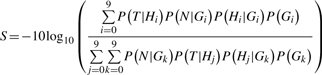
To detect somatic mutations, we calculate the likelihood that a site is not somatic as follows. Given data from the tumor T and the normal N and genotypes G , we calculate a somatic score S as:

Where the genotype likelihood is P(D|G_i|), D is the data in either tumor or normal and where P(D|G_i|) is any of 10 possible diploid genotypes (i.e. AA, AC, AG, AT, CC, CG, CT, GG, TT). For the genotype, the subscript l indexes into this list (e.g. G₀=AA). We calculate the genotype likelihood using the MAQ algorithm and the prior probability P(G₁) is calculated as follows:

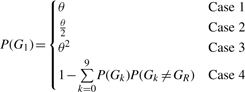where θ is the expected rate of heterozygous mutations in the population of interest and G_R is the reference base at the position of interest (Li et al., 2009b). We use a value of θ=0.001 for human samples. Case 1 occurs when the genotype is heterozygous, but shares an allele with the reference. For example, the reference is A and G_l=AG. Case 2 occurs when the genotype is homozygous variant. Case 3 occurs when the genotype is heterozygous, but shares no alleles with the reference base. For example, if the reference is A and G_l=CG. Lastly, Case 4 occurs when the genotype is homozygous for the reference base.

This initial derivation is equivalent to comparing the probabilities of the two mutations as independent germline mutations. Thus, any correlation between the two samples is not explicitly accounted for. In addition, we provide the option to use uniform prior probabilities.

Previous validation results within our institute indicated that very few valid somatic mutations have a somatic score <15 (data not shown) and, therefore, we do not typically report any sites with a score below this number. In addition, we exclude randomly mapped reads (mapping quality 0) from contributing to mutation calls.

2.1.2 Derivation utilizing somatic mutation rate

The initial derivation above assumes that the tumor and normal genotypes are independent. Since these two samples are from a single individual, a better derivation, taking into account the dependence of the tumor and normal genotypes on each other, is:

In this equation, G is the genotype in the normal and is defined identically as before and H is the genotype in the tumor. The probability P(H_m|G) takes into account the prior probability of a somatic mutation, μ, for a given normal genotype, G, as follows:

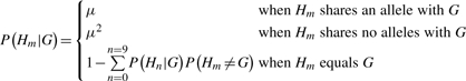A value for μ of 0.01, which is much larger than observed somatic mutation rates in tumors (Greenman et al., 2007), yields similar results to the original equation. When evaluating this derivation, we use the same minimum somatic score cutoff of 15, though we note that at lower values of μ this may no longer be appropriate.

2.2 Standard somatic detection filters

Our standard pipeline (Ding et al., 2010; Mardis et al., 2009) for identifying candidate somatic mutations consists of several steps to filter calls with respect to errors unaccounted for in the MAQ genotyping model. We initially filter using Samtools (Li et al., 2009a) calls from the tumor. Sites are retained if they meet all of the following rules inspired by MAQ (Li et al., 2008):

1. Site is >10 bp from a predicted indel of quality ≥50.

2. Maximum mapping quality at the site is ≥40.

3. Fewer than three SNV calls in a 10 bp window around the site.

4. Site is covered by at least three reads.

5. Consensus quality ≥20.

6. Single Nucleotide Polymorphism (SNP) quality ≥20.

SomaticSniper predictions passing the filters are then intersected with calls from dbSNP build 130 (Sherry et al., 2001) and sites matching both the position and allele of known dbSNPs are removed. Sites where the normal genotype is heterozygous and the tumor genotype is homozygous and overlaps with the normal genotype are removed as probable loss of heterozygosity events.

Lastly, we empirically classify our mutations into two bins based upon our validation experiences (data not shown). We define a high confidence (HC) mutation as a site where the reads supporting the variant have an average mapping quality ≥40 for BWA (or 70 for MAQ) and the somatic score is ≥40.

2.3 Simulation of variant sites

In order to evaluate the software on theoretical data, we implemented a simple simulation method to generate 10 000 variants. We simulated 1 bp reads covering each variant with a mapping quality of 60, a base quality of 30 and various variant allele frequencies. Variant bases were generated by sampling from a binomial distribution with expectation equal to the simulated allele frequency. Base errors were introduced at a rate equal to the base quality. The probability that the base error was reported as any particular incorrect base was uniform.

2.4 Training and use of SNVMix2

We sought to compare the sensitivity of SomaticSniper with that of another SNV caller, SNVMix2 (Goya et al., 2010). To train SNVMix2 for calling, we obtained Affymetrix Genome Wide SNP 6 microarray data from the Wellcome Trust Sanger Institute Cancer Genome Project website, http://www.sanger.ac.uk/genetics/CGP, and called genotypes using the default options of the CRLMM R package (Carvalho et al., 2010). We retained genotypes receiving a confidence score >0.99 and extracted the position of each probe using version 30 of the Genome Wide SNP 6.0 from Affymetrix. We then reduced the number of calls by randomly removing 98% of them in order to reduce our number to a similar scale as used for training SNVMix previously (Goya et al., 2010). This left 17 469 sites for the normal and 16 761 sites for the tumor. We generated tallies of the spanning reads for these sites (pileup) for each sample using Samtools and used the pileup output to train a SNVMix2 model for each sample.

We ran SNVMix2 using the models generated by training on the microarray data. Since SNVMix2 is, at its core, a single genome caller, we implemented a comparison of the probabilities produced to generate a somatic score analogous to the score calculated by SomaticSniper. For sites in the tumor called as a variant by SNVMix2 and receiving a call in the normal, we calculated a somatic probability as follows:

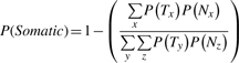where T is the genotype in the tumor sample and N is the genotype in the normal sample as called by SNVMix2. Each genotype is drawn from three distinct diploid possibilities x,y,z={aa,ab,bb} where a is the reference allele and b the variant allele. We report any sites where P(Somatic) ≥0.9 as a somatic call by SNVMix2.

3 RESULTS

As a result of our work sequencing leukemia genomes, we developed a method for identifying potentially somatic mutations. Our algorithm, previously referred to as glfSomatic (Ding et al., 2010; Mardis et al., 2009), explicitly calculates the likelihood of genotype difference between two genomes at all positions with coverage in both and reports variants in the tumor along with a somatic score, a Phred-scaled value indicating the likelihood that the site is not somatic.

3.1 Performance on simulations

Samples of tumors, and potentially normals, are heterogeneous populations of both tumor and normal cells. To evaluate the theoretical upper bound on the performance of our algorithm, we tested its ability to detect simulated heterozygous mutations across a wide range of abundances. We held mapping quality, base error rate and sequencing depth in both tumor and normal constant and evaluated the number of variants called with the variant base at each position. For allele frequencies that are clearly somatic, these simulations yield an estimate of our power to detect variants at those abundances. For simulations of roughly equal allele frequencies, the number of called variants gives an estimate of the false positive rate.

Our simulations show that at a depth of 30X in both tumor and normal, the algorithm is powered to detect 90% of mutations for tumor allele frequency >30% if the normal is completely pure (Fig. 1A). In cases such as leukemia, where there are frequently tumor cells mixed in with the normal sample, power is still >90% for tumor variant allele frequencies >35% and normal variant allele frequencies of ≤slant 5%. Higher variant allele frequencies in the normal rapidly diminish our predicted power with frequencies of 10% essentially capping the power at 67% and reducing it to <5% at or above normal allele frequencies of 20%. This reduction occurs even at very high tumor allele frequencies.

Fig. 1.

Simulations of power across various variant allele frequencies and across different depths in both samples: 30 reads (A), 60 reads (B) and 90 reads (C). Contours indicate the power for each combination of variant allele frequencies. The dashed line indicates simulations where the allele frequencies in tumor and normal are equal and thus, the contours intersecting this line indicate the expected FDR for those allele frequencies.

We also conducted simulations at higher depths of 60X and 90X and found that, for highly pure tumor and normal samples, our power increased with depth allowing for >90% sensitivity for mutations present at 25% allele frequency with 90X depth (Fig. 1B and C). In contrast, while our power increased for normal allele frequencies <10%, it was reduced for normal allele frequencies above ~15%. Thus, higher depth increases power for cases where the normal sample is relatively pure, but reduces it for impure normal samples. Simulations using uniform prior probabilities showed an increase in sensitivity for pure samples, but reduced sensitivity for impure samples (Supplementary Fig. S1A–C). With somatic prior probabilities, we observed similar trends with a somatic prior probability of 0.01, but observed a large reduction in the power of detection at 30X depth when using a somatic prior of μ=0.000001 which is much closer to the somatic mutation rate of adult tumors (Supplementary Fig. S1D–I).

The estimated false discovery rate (FDR) remained ≤15% across all depths and frequency combinations, but peaked for variants at ~15% frequency in both tumor and normal (Fig. 1). In contrast, the simulations showed a lower FDR with either uniform prior probabilities or somatic prior probabilities (Supplementary Fig. 1). Using the more realistic somatic prior probability of μ=0.000001 resulted in a sub-10% FDR (Supplementary Fig. S1G–I).

3.2 Estimation of sensitivity on real data

While we have evaluated SomaticSniper on a large number of cancer genomes within our institute, we sought also to test its sensitivity on an external dataset, as well as to compare its performance to pre-existing tools. To evaluate sensitivity, we used the recently published sequence data of a melanoma cell line (Pleasance et al., 2010a), having obtained these data for both the tumor and normal cell lines from the Wellcome Trust Sanger Institute Cancer Genome Project via the European Bioinformatics. Out of 497 previously validated sites, we called 496 for a sensitivity of 99.8%. Visual inspection of the single uncalled site showed a low variant allele frequency of 23% and many low-quality bases (mean base quality of 15.22). Our complete pipeline with standard filters resulted in substantial filtering of calls with only a modest decrease in sensitivity (Table 1).

Table 1.

Sensitivity estimation on COLO-829 data

Program	Filtering	Total calls	Called from Pleasance (sensitivity), n (%)	COSMIC only (sensitivity), n (%)
SomaticSniper	None	636 467	496 (99.8)	77 (92.8)
SomaticSniper	Standard	111 239	490 (98.6)	74 (89.2)
SomaticSniper	HC + standard	43 875	488 (98.2)	73 (88.0)
SomaticSniper	Standard + additional	53 489	468 (94.2)	73 (88.0)
SomaticSniper	Standard + additional + HC	36 489	466 (93.8)	72 (86.8)
SNVMix2	None	772 301	493 (99.2)	75 (90.4)

Since the estimated sensitivity of the Pleasance study was ~88% and the majority of reported variants came from that particular study, we also examined our performance on sites in COSMIC (Forbes et al., 2011) where the WGS study was not the sole source of the mutation. Of the 83 somatic sites in this set, 77 were called by SomaticSniper for a sensitivity of 92.3%. The sites that were missed either had a variant frequency <20% (three sites <20%) or an average variant base quality <20 combined with a variant frequency <30% (two sites). For our complete pipeline, we again saw only a modest reduction of sites for an overall sensitivity of 89.2% in this dataset (Table 1).

We also ran SNVMix2 on the same dataset for comparison purposes. SNVMix2 is a single genome caller that has been developed for the identification of somatic mutations in other studies, albeit not for direct comparison of tumor/normal pairs (Goya et al., 2010). SNVMix2 generated a similar number of calls as unfiltered SomaticSniper and showed a comparable sensitivity (Table 1). There was a large amount of overlap between the two call sets with 537 522 calls being shared between the two and 234 779 unique to SNVMix2 and 98 945 unique to SomaticSniper.

3.3 Estimation of precision

We recently completed the sequencing of a relapse tumor sample from an earlier Acute Myeloid Leukemia (AML) case (L.Ding et al., submitted for publication). This genome had 34.2X coverage in the relapse and 26.2X coverage in the matched normal. We predicted variants from these data using SomaticSniper with uniform prior probabilities. These calls should provide a conservative estimate of the precision of the algorithm, as validation for other samples indicated that calls made with uniform priors validate at a lower rate than those with the standard priors (data not shown). We used solid phase capture (Nimblegen) to pull down predicted variants and then re-sequenced the captured fragments using the Illumina GAIIx platform to generate deep coverage (mean depth across targets of 1065X for the normal and 520X for relapse). A small number of variants that failed to meet these criteria, which we had previously validated as somatic, were also targeted, but are not included in this work. The resulting data were used to assemble a set of true variants to estimate precision. To obtain independently verified results, we used VarScan2 (Koboldt et al., 2009) as an orthogonal caller, a minimum coverage requirement of 30 reads in each sample, and a P-value cutoff of 0.001 to determine the somatic status of each mutation.

We attempted to validate 1018 mutations in coding, non-coding RNA, potentially regulatory and non-repetitive regions of the genome according to our standard partitioning (Ding et al., 2010; Mardis et al., 2009). This set contained predictions of both high and low confidence bins for sites falling within coding and non-coding transcripts, but the remaining mutations were drawn solely from the HC bin. VarScan identifies variants based on coverage and observed allele frequency, and assigns them to one of three categories based on a Fisher's exact test of the read counts supporting each allele: Reference, indicating there is no variant at this site in either tumor or normal; Germline, indicating there is a single variant present in both tumor and normal (P≥0.001); and Somatic, indicating there is a tumor specific variant at the site (P<0.001). We obtained sufficient coverage for 930 sites, from which 384 sites were called as Somatic. Thus, we observed a net validation rate of 37.7% and a covered validation rate of 41.3% (Table 2). The false positives were divided among 504 Reference calls and 33 Germline calls. Nine sites were called Somatic but did not meet our P-value cutoff.

Table 2.

Estimation of SomaticSniper precision

Sample	Tumor type	Filter	Target regions	Assays designed	Successful assays	Validated	Maximal sensitivity, %	Precision, %
933 124	AML	Standard	1018	1000	930	384	100	37.7
933 124	AML	Standard + review	1018	1000	930	376	100	36.9
933 124	AML	Additional	493	486	480	372	98.9	75.5
16 319	Breast	Standard	5578	5542	5499	4702	100.00	84.30
16 319	Breast	Additional	5290	5273	5243	4689	99.72	88.64
16 347	Breast	Standard	860	841	818	546	100.00	63.49
16 347	Breast	Additional	684	678	667	545	99.82	79.68
16 454	Breast	Standard	2430	2401	2346	1798	100.00	73.99
16 454	Breast	Additional	2117	2103	2073	1775	98.72	83.85

We also attempted to evaluate the sensitivity and precision using a somatic prior probability of 0.01 on this data. This resulted in somewhat fewer calls with a sensitivity of 98.9%. In addition, a large bin of novel calls (228) was present after standard filtering. We reviewed these calls and identified likely somatic mutations in this set. Were all these novel predictions to validate, our precision with this alternate method would be 48.3% (Supplementary Table S1).

3.4 Frequent sources of false positives

Our simulation results predicted a maximal FDR of ~15% in the absence of mapping errors and in the presence of perfectly calibrated base qualities. Since neither of these assumptions is true for real data, we expected a higher FDR than the simulations and we sought to identify any systematic errors that might cause false positive predictions. Since the validation identified 537 clear false positive sites, we examined the original WGS data for sites that did not validate in the capture data. We observed several indicators that a site was likely to be a false positive that were borne out by more detailed analysis and were developed into several filters to improve the overall validation rate.

3.4.1 Strand bias

One major indicator of a false positive is strand bias, where the variant allele arises primarily from reads aligning on one strand versus the other. We examined the strand distribution, as the fraction of variant supporting reads mapping to the plus strand, for each of the three variant classes arising from our validation experiment. We found that the reference calls were enriched for sites strongly biased toward one direction or the other (Supplementary Fig. S2).

3.4.2 Effective 3^′ end

Beginning with version 1.5, the Illumina pipeline uses the Read Segment Quality Control Indicator to identify 3^′ portions of reads that should be discarded. This is done by setting the base quality for the region to 2 and we will henceforth refer to such a region as a Q2 region. We have observed that false positive bases of high quality frequently occur near these regions. Since not every read has a Q2 region and Q2 regions may be removed by quality trimming, we defined a measurement we call the distance to the effective 3^′ end (DETPE), which equals the smallest distance between the variant base and either the 3^′ end of the read, the 3^′ clipped end or the 5^′ end of the Q2 run normalized by the unclipped read length.

The distribution of this measure on our data hovered at ~0.46 as assessed in reads containing heterozygous SNVs from microarray data for known germline variants (Supplementary Fig. S3). We then examined the distributions in the original data for this attribute and found that variants that validated as Reference tended to be associated with a small DETPE (Fig. 2A). In addition, we found that this measure was positively correlated with the aforementioned strand bias (Pearson's correlation of 0.31). In contrast, association of the variant bases with the physical 3^′ end of the read indicated little bias between classes (Fig. 2B).

Fig. 2.

Association of erroneous calls with the effective 3^′ end. Kernel density estimates comparing the distribution of two different measures of variant location across three different validation results. The bandwidth (bw) for each kernel density is shown in the legend. (A) Variants that validated reference show a clear bias toward association with the effective 3^′ end. (B) All three classes of validated mutations show no clear bias in association with the end of the sequenced read.

3.4.3 Homopolymers and paralogs

We found two remaining sources of error: variant bases that appeared to be generated from read-through of homopolymer runs and reads that appeared to map from paralogs not in the reference. To identify reads that might support a paralog, we quantified the number of mismatches in a given read by summing the base qualities of the mismatches up for a given read the mismatch quality sum (MMQS). This is similar to what is done in MAQ (Li et al., 2008). Since introduction of a somatic mutation within a read length from a germline mutation on the same chromosome would result in a higher MMQS, we compared the MMQS for reads containing the variant in the tumor to the normal directly. We found an enrichment among the false positive sites in both germline and reference classes for a high MMQS difference (Supplementary Fig. S4). In addition, we examined both the maximum and sum of the number of adjacent bases identical to the variant base in both 5^′ and 3^′ directions. Inspection showed clear biases in the data for these features (Supplementary Fig. S5).

3.5 Application of additional filters

Based on these observations, we implemented filters that should apply to 100 bp read length data. We calculated a stranded bias P-value under the null hypothesis that reads are expected to be sampled equally from each strand as a binomial model with ‘success’ taken arbitrarily as a read mapping to the forward strand. For calculating the bias of the variant base's distance to the effective 3^′ end, we applied a Kolmogorov–Smirnov (KS) test using a reference distribution built from true heterozygous germline SNPs as determined by SNP array. We then used the beta approximation of the KS test (Zhang and Wu, 2002) to calculate the DETPE P-value. If both P-values were <0.1, we filtered the variant. We also made some simple heuristic filters on the MMQS difference and homopolymer difference based on the observed distributions. We removed potential homopolymer errors by removing variants flanked by homopolymers of length >3 or surrounded by >6 identical bases. Based on the empirical distribution of MMQS, we removed variants with a MMQS difference of ≥60.

After determining appropriate filters, we sought to evaluate their performance on both of our testing datasets. Applying all of the above filters to the original whole genome data from our leukemia dataset (L.Ding et al., submitted for publication) removed 525 mutations, including 12 called somatic mutations. Upon manual review, eight of these called somatic mutations were actually false positives as was one additional somatic mutation that passed all filters (Table 2). If these filters had been applied to the original data, then we would have increased our precision to 75.5% and observed a decrease in sensitivity of at most 1.1% (Table 2).

To verify that these filters were not over-fitted to our training set, we applied them to the COLO-829 data (Pleasance et al., 2010a) as well as three breast cancer genomes from our recent sequencing of 46 breast cancer tumors (M.J.Ellis et al., submitted for publication). For COLO-829, application of the additional filters resulted in nearly half as many calls, but only a decrease in sensitivity of at most 4.4%. Similar results were observed on the COSMIC sites (Table 1). For the three breast cancer genomes, somatic variants were called and validated identically to our leukemia dataset as described above. We observed a precision of between 64% and 84% before additional filtering. Application of the additional filters increased the precision in all cases to between 79% and 89% with an accompanying maximal decrease in sensitivity between 0.2% and 1.2% (Table 2). Thus, we infer that the proposed filters are not over-fitted to the AML data and are generally applicable to somatic predictions.

4 DISCUSSION

The detection of somatic SNVs in tumors is an important part of tumor resequencing because these mutations can be directly relevant to the disease and are the most numerous. One method of discovering somatic SNVs is to compare the sequencing results between a matched tumor and normal pair. To this end we developed SomaticSniper to directly compare the tumor and normal reads and calculate the probability that the two samples have identical genotypes in both samples.

Our simulations on the algorithm show that it should be able to detect most mutations if the mutation is present in the majority of cells, and the normal is relatively pure. We have evaluated SomaticSniper on external data and found it to be more sensitive than other methods and, based on the total number of calls, of comparable specificity. Additionally, we have explored the precision of our algorithm by validating predicted somatic mutations on internally generated data. In contrast to our simulations, which suggested an FDR <15% if mapping error is non-existent, this validation experiment demonstrated a higher FDR. Our subsequent investigations revealed a number of reliable indicators that a predicted variant was, in fact, not real. Most interestingly, we identify an association of false positive bases with the Illumina Q2 base quality designation. This new feature may also prove useful in other false positive reduction techniques, such as base quality recalibration. By implementing some statistical and empirical filters, we were able to greatly increase the validation rate on both our training set and four independent datasets with only a small number of validated somatic mutations failing the filters. While our precision is low on the AML sample, this is expected since there are a smaller number of detectable events due to both tumor cells in the normal sample and a lower mutation rate for this cancer type. In solid tumors, where neither problem is likely to be as severe, we expect that the precision should be similar to that observed on the tested breast cancer tumors.

Despite the success of SomaticSniper on the COLO-829 data, this dataset represents an ideal case for somatic SNV calling and there remains room for improvement in future work. Since COLO-829 is a cell line, it represents the simple case of a perfectly pure, homogenous tumor with a perfectly pure, homogenous matched normal. Cancer projects will rarely work with such an ideal sample and tumors can be expected to contain multiple subclones with varying expected allele frequencies depending on their site-specific copy number and abundance within the tissue sample. Indeed, the internal data with which we evaluated our precision were obtained from a patient with a high white blood cell count (105 000 cells per microliter) and our data indicate that ~30% of the cells from the normal sample were, in fact, tumor (Ley et al., 2008). In addition, the tumor sample will likely be impure in many cases. While the matched normal can be expected to be free of tumor cells for most samples, this may not always be the case (especially for liquid tumors that circulate into all tissues, and for solid tumors where the matched normal tissue is obtained from adjacent tissue).

Our simulation studies demonstrate the rapid decline of detection power that occurs when the normal sample contains tumor cells. This is due, in part, to the assumptions of the MAQ genotyping model underlying SomaticSniper, which currently operates by ignoring the copy number state and sample purity. This is true for SNVMix2 as well, since it derives its expected genotype frequencies from training on germline variants. Optionally, our caller can take into account the prior knowledge that somatic SNVs are expected to be rare, although our testing suggests that incorporating such a penalty significantly reduces the sensitivity of the algorithm at current WGS coverage levels (Supplementary Fig. S1). As outlined above, these assumptions are inappropriate for optimal somatic SNV calling and future improvements in somatic SNV calling must take these issues into account.

Sites predicted to be somatic by our method will include both true mutations and some false positives. The number of false positives is likely to be a function of the quality of the reference sequence, the alignments, the data quality and the ability to accurately provide error estimates to the software. While our filters increase precision, fully specified error models or adjustments to the error estimates provided in the mapping qualities and base qualities of the data ought to improve the specificity and sensitivity of these filters.

REFERENCES

- Carvalho B.S., et al. Quantifying uncertainty in genotype calls. Bioinformatics. 2010;26:242–249. doi: 10.1093/bioinformatics/btp624. [DOI] [PMC free article] [PubMed] [Google Scholar]
- Ding L., et al. Genome remodelling in a basal-like breast cancer metastasis and xenograft. Nature. 2010;464:999–1005. doi: 10.1038/nature08989. [DOI] [PMC free article] [PubMed] [Google Scholar]
- Forbes S.A., et al. COSMIC: mining complete cancer genomes in the Catalogue of Somatic Mutations in Cancer. Nucleic Acids Res. 2011;39:D945–D950. doi: 10.1093/nar/gkq929. [DOI] [PMC free article] [PubMed] [Google Scholar]
- Goya R., et al. SNVMix: predicting single nucleotide variants from next-generation sequencing of tumors. Bioinformatics. 2010;26:730–736. doi: 10.1093/bioinformatics/btq040. [DOI] [PMC free article] [PubMed] [Google Scholar]
- Greenman C., et al. Patterns of somatic mutation in human cancer genomes. Nature. 2007;446:153–158. doi: 10.1038/nature05610. [DOI] [PMC free article] [PubMed] [Google Scholar]
- Jones S., et al. Frequent mutations of chromatin remodeling gene ARID1A in ovarian clear cell carcinoma. Science. 2010;330:228–231. doi: 10.1126/science.1196333. [DOI] [PMC free article] [PubMed] [Google Scholar]
- Koboldt D.C., et al. VarScan: variant detection in massively parallel sequencing of individual and pooled samples. Bioinformatics. 2009;25:2283–2285. doi: 10.1093/bioinformatics/btp373. [DOI] [PMC free article] [PubMed] [Google Scholar]
- Ley T.J., et al. DNA sequencing of a cytogenetically normal acute myeloid leukaemia genome. Nature. 2008;456:66–72. doi: 10.1038/nature07485. [DOI] [PMC free article] [PubMed] [Google Scholar]
- Ley T.J., et al. DNMT3A mutations in acute myeloid leukemia. N. Engl. J. Med. 2010;363:2424–2433. doi: 10.1056/NEJMoa1005143. [DOI] [PMC free article] [PubMed] [Google Scholar]
- Li H., et al. Mapping short DNA sequencing reads and calling variants using mapping quality scores. Genome Res. 2008;18:1851–1858. doi: 10.1101/gr.078212.108. [DOI] [PMC free article] [PubMed] [Google Scholar]
- Li H., et al. The Sequence Alignment/Map format and SAMtools. Bioinformatics. 2009a;25:2078–2079. doi: 10.1093/bioinformatics/btp352. [DOI] [PMC free article] [PubMed] [Google Scholar]
- Li R., et al. SNP detection for massively parallel whole-genome resequencing. Genome Res. 2009b;19:1124–1132. doi: 10.1101/gr.088013.108. [DOI] [PMC free article] [PubMed] [Google Scholar]
- Mardis E.R., et al. Recurring mutations found by sequencing an acute myeloid leukemia genome. N. Engl. J. Med. 2009;361:1058–1066. doi: 10.1056/NEJMoa0903840. [DOI] [PMC free article] [PubMed] [Google Scholar]
- Pleasance E.D., et al. A comprehensive catalogue of somatic mutations from a human cancer genome. Nature. 2010a;463:191–196. doi: 10.1038/nature08658. [DOI] [PMC free article] [PubMed] [Google Scholar]
- Pleasance E.D., et al. A small-cell lung cancer genome with complex signatures of tobacco exposure. Nature. 2010b;463:184–190. doi: 10.1038/nature08629. [DOI] [PMC free article] [PubMed] [Google Scholar]
- Shah S.P., et al. Mutation of FOXL2 in granulosa-cell tumors of the ovary. N. Engl. J. Med. 2009a;360:2719–2729. doi: 10.1056/NEJMoa0902542. [DOI] [PubMed] [Google Scholar]
- Shah S.P., et al. Mutational evolution in a lobular breast tumour profiled at single nucleotide resolution. Nature. 2009b;461:809–813. doi: 10.1038/nature08489. [DOI] [PubMed] [Google Scholar]
- Sherry S.T., et al. dbSNP: the NCBI database of genetic variation. Nucleic Acids Res. 2001;29:308–311. doi: 10.1093/nar/29.1.308. [DOI] [PMC free article] [PubMed] [Google Scholar]
- Wendl M.C., Wilson R.K. Aspects of coverage in medical DNA sequencing. BMC Bioinformatics. 2008;9:239. doi: 10.1186/1471-2105-9-239. [DOI] [PMC free article] [PubMed] [Google Scholar]
- Wiegand K.C., et al. ARID1A mutations in endometriosis-associated ovarian carcinomas. N. Engl. J. Med. 2010;363:1532–1543. doi: 10.1056/NEJMoa1008433. [DOI] [PMC free article] [PubMed] [Google Scholar]
- Zhang J., Wu Y.H. Beta approximation to the distribution of Kolmogorov-Smirnov statistic. Ann. Ins. Stat. Math. 2002;54:577–584. [Google Scholar]
Associated Data
This section collects any data citations, data availability statements, or supplementary materials included in this article.