Trajectory Approach to Two-State Kinetics of Single Particles on Sculpted Energy Landscapes

Abstract

We study the trajectories of a single colloidal particle as it hops between two energy wells which are sculpted using optical traps. Whereas the dynamical behaviors of such systems are often treated by master-equation methods that focus on particles as actors, we analyze them instead using a trajectory-based variational method called maximum caliber (MaxCal). We show that the MaxCal strategy accurately predicts the full dynamics that we observe in the experiments: From the observed averages, it predicts second and third moments and covariances, with no free parameters. The covariances are the dynamical equivalents of Maxwell-like equilibrium reciprocal relations and Onsager-like dynamical relations.

We explore the kinetics of two-state processes, A ⇌ B, at the one-particle level. Examples of single-molecule or single-particle dynamical processes that mimic this two-state dynamics include DNA loop formation [1], protein folding oscillations [2], or ion-channel opening and closing kinetics [3]. Two-state fluctuating systems having fixed rates are called random-telegraph processes.

One way to understand two-state and random-telegraph processes is through master equations, which are differential equations that are solved for time-dependent probability density functions [4]. For single-particle and few-particle systems, however, other convenient experimental observables are the trajectories themselves rather than the time-dependent populations of the two states. Here we describe an experimental model system to study such single-particle two-state stochastic trajectories. We use these experiments to test a theoretical strategy, called maximum caliber, that provides a way to predict the full trajectory distributions, given certain observed mean values. It has not yet been much tested experimentally; that is the purpose of the present work.

Using dual optical traps, we have “sculpted” various energy landscapes. We can control the relative time the particle spends in its two states and the rate of transitioning between them. Our method follows from earlier work on the dual trapping of colloidal particles that was used to study Kramers reaction rate theory [5]. While these experiments were previously focused on studying average rates, our interest here is in the probability distribution of trajectories.

We trap a 1 μm silica bead in a neighboring pair of optical traps. The laser at 532 nm, 100 mW, provides an inverted double-Gaussian shaped potential. An acousto-optic deflector alternately sets up two traps close together in space, at a switching rate of 10 kHz, which is both much faster than each individual trap's corner frequency [6] and also the fastest bead hopping rate. The strength of each trap and the spacing between them can be controlled in order to sculpt the shape of the potential. A tracking 658 nm red laser at 1 mW was used to determine the position of the bead. The forward scattered light is imaged through a microscope condenser onto a position-sensitive detector [7]. The green trapping laser light at the detector is filtered out by a long-pass filter. The data were recorded at a rate of 20 kHz, which sets the fundamental time step Δt for our analysis. Trajectories were recorded for intervals ranging from 20 minutes to more than 1 hour, depending on the hopping rate. A simple threshold was used to determine states in the trajectories.

First proposed by Jaynes in 1980, maximum caliber (MaxCal) is a variational principle that purports to predict dynamical properties of systems in much the same way that the maximum entropy (MaxEnt) approach predicts the properties of equilibrium systems; both use information theory as a basis [8]. MaxCal has been shown to be a simple and useful way to derive the flux distributions in diffusive systems, such as in Fick's law of particle transport, Fourier's law of heat transport, and Newton's viscosity law of momentum transport [9]. The algorithm of MaxCal is identical to that of MaxEnt. As a reminder, MaxEnt augments the Shannon entropy S = Σ_sp_s ln p_s, where p_s denotes the probability of a state s (using the technique of Lagrange multipliers), with moment quantities that are conserved within the chosen ensemble; maximizing the entropy produces the probability distribution of states in equilibrium. In MaxCal, an entropylike quantity taking on the same C = Σ_ip_i ln p_i form, where C is the caliber and p_i denotes the probability of the ith trajectory, is also augmented with moment-type quantities which are in fact experimental observables. Maximization of the caliber thus predicts the full distribution of trajectories. Thus MaxCal plays the same role for dynamics that MaxEnt plays for equilibrium.

Examples of trajectories in our system are shown in Fig. 1. By trajectory, we mean one individual time sequence of events over which the particle can transition back and forth many times between states A and B. In our experiments, we divide time into discretized time intervals Δt set by the inverse of our sampling rate. A trajectory has N time steps, so it lasts for a total time NΔt. We aim to characterize the probability distribution for all trajectories given the known constraints on the space of possible trajectories, as defined by our first-moment experimental observables.

Fig. 1.

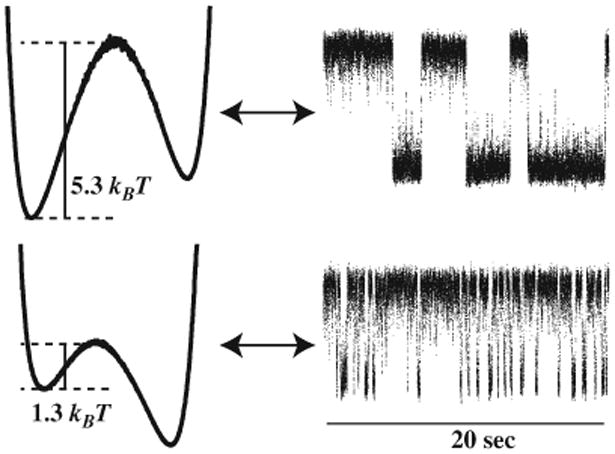
Sculpted energy landscapes (left, averaged 20 minutes) and the corresponding microtrajectories. The trace is raw data; states are assigned after boxcar filtering and threshold finding. Top: The lower state is slightly more populated; there is a high barrier (infrequent transitions). Bottom: The upper state is more populated; the barrier is small (frequent transitions). The distance between the two potential minima ranges from 200 to 700 nm.

We take a reduced view of the experimental system which will allows the solution to p_i to be analytically tractable. For each Δt time step, there are four possible transitions. If the system is in state a, it can stay in state a or switch to state b. Similarly, if the system is in state b, it can stay in state b or switch to state a. Over the entirety of the ith trajectory, the total number of transition events from a to a is represented by the variable N_aa, with N_ab, N_ba, and N_bb defined similarly. In the experiments, the observables are the averages of these quantities, 〈N_ab〉, 〈N_ba〉, 〈N_aa〉, and 〈N_bb〉, taken over all of the trajectories [summarized in Eqs. (3) and (4)]. Thus there are four corresponding unknown Lagrange multipliers (plus normalization) which are fully determined by the four observables. In this case, the caliber is defined as C = −Σ_i[p_i ln p_i − λ₀ p_i − p_i(λ_aaN_aa,i − λ_abN_ab,i − λ_baN_ba,i − λ_bbN_bb,i)], where the λ's are the corresponding Lagrange multipliers. [Among this set of five Lagrange multipliers, there are only two independent variables (see below), so only two experimental average quantities are required [10]]. The probabilities p_i of all of the trajectories are then found by maximizing the caliber $\frac{\partial c}{\partial p_i}=0$.

The calculation of the p_i's is made simple by the use of the trajectory partition function Q_d, which serves for our dynamical system very much the same role that the equilibrium partition function serves for the Boltzmann distribution law of equilibrium. For 2^N trajectories having N time steps, Q_d is given by

$$Q_d=\sum _i^{2N}\left({\alpha }^{N_{aa,i}}{\beta }^{N_{bb,i}}{\omega }_f^{N_{ab,i}}{\omega }_r^{N_{ba,i}}\right),$$ (1)

and the probability of a particular trajectory labeled i is given by

$$p_i=Q_d^{-1}{\alpha }^{N_{aa,i}}{\beta }^{N_{bb,i}}{\omega }_f^{N_{ab,i}}{\omega }_r^{N_{ba,i}}.$$ (2)

We write the exponentiated Lagrange multipliers as the “statistical weights” α, β, ω_f, and ω_r, with respect to the observables described above: α is the statistical weight that, given that the system is in state A at time t, it is also in state A at time t + Δt; β, for staying in state B at time t + Δt, given that the system was in B at time t; ω_f, for switching from A to B in the time interval Δt; and ω_r, for switching from B to A in the time interval Δt.

It is readily shown that the average quantities are simply derivatives of the partition function; for example,

$$\langle N_{bb}\rangle ={\frac{\partial ln{Q}_d}{\partial ln\beta }|}_{\alpha ,{\omega }_f,{\omega }_r},\langle N_{ab}\rangle ={\frac{\partial ln{Q}_d}{\partial ln{\omega }_f}|}_{\alpha ,\beta ,{\omega }_r}$$ (3)

and

$$\langle N_{aa}\rangle ={\frac{\partial ln{Q}_d}{\partial ln\alpha }|}_{\beta ,{\omega }_f,{\omega }_r},\langle N_{ba}\rangle ={\frac{\partial ln{Q}_d}{\partial ln{\omega }_r}|}_{\alpha ,\beta ,{\omega }_f}$$ (4)

together define the statistical weights.

The MaxCal strategy is as follows. First, experiments give the four trajectory-averaged quantities such as 〈N_bb〉, 〈N_ab〉, etc. Second, substituting those measured values into Eqs. (3) and (4) gives four equations that are solved for the four unknowns α, β, ω_f, and ω_r. This now gives all of the information needed to compute Q_d and p_i for any trajectory from Eqs. (1) and (2). Finally, taking the second and higher derivatives of Q_d gives the higher moments (i.e., the dynamical fluctuations) of the observables, such as $\langle N_{ba}^2\rangle -{\langle N_{ba}\rangle }^2={\frac{{\partial }^{2}ln{Q}_d}{\partial {\left(ln{\omega }_r\right)}^2}|}_{\alpha ,\beta ,{\omega }_f}$.

In addition, other properties of interest are also readily computed. Let N_B represent the number of units of time that the system spends in state B. Then we have for each individual trajectory N_B = N_ab + N_bb + N_0b and N_A = N_aa + N_ba + N_0a, where N_0b is 0 (1) if the trajectory begins in state A (B) and N_0a is 1 (0) if the trajectory begins in state A (B). If the number of steps is sufficiently large, the contribution from initial conditions can be ignored. Hence the variance for N_B is given by $\langle N_B^2\rangle -{\langle N_B\rangle }^2\simeq {\frac{{\partial }^{2}ln{Q}_d}{\partial {\left(ln\beta \right)}^2}|}_{\alpha ,{\omega }_r,{\omega }_f}+{\frac{{\partial }^{2}ln{Q}_d}{\partial {\left(ln{\omega }_f\right)}^2}|}_{\alpha ,\beta ,{\omega }_r}+2{\frac{{\partial }^{2}ln{Q}_d}{\partial ln\beta \partial ln{\omega }_f}|}_{\alpha ,{\omega }_r}$.

Mixed moments and covariances are obtained from mixed derivatives of Q_d. For example,

$${\frac{{\partial }^{2}ln{Q}_d}{\partial ln{\omega }_f\partial ln\beta }|}_{\beta ,{\omega }_r}={\frac{{\partial }^{2}ln{Q}_d}{\partial ln\beta \partial ln{\omega }_f}|}_{\alpha ,{\omega }_r},$$ (5)

which leads to ${\frac{\partial \langle N_{bb}\rangle }{\partial ln{\omega }_f}|}_{\alpha ,\beta ,{\omega }_r}={\frac{\partial \langle N_{ab}\rangle }{\partial ln\beta }|}_{\alpha ,{\omega }_f,{\omega }_r}=\langle N_{ab}{N}_{bb}\rangle -\langle N_{ab}\rangle \langle N_{bb}\rangle$. Higher derivatives of Q_d give information about the higher-order fluctuations. Hence, given Q_d, all of the trajectory observables and their moments can be computed. More details of the theoretical approach for this problem are given in Ref. [10].

A simple way to compute Q_d is through the matrix propagator G:

$$\mathbf{\text{G}}=\left(\begin{array}{cc}\alpha & {\omega }_r\\ {\omega }_f& \beta \end{array}\right),$$ (6)

where each element of G represents the statistical weight of transitioning from some initial state during each time step. We consider here only stationary processes, for which the statistical weights are time-independent, but the MaxCal method itself is not limited to such simple dynamics. We can express Q_d = (11)G^N−1(a₀ b₀)^T, where (a₀ b₀)^T denotes the initial state probabilities. Thus all of the higher moments of the observables are analytically tractable since Q_d can always be expressed in terms of partial derivatives of the eigenvalues of G. For nonstationary processes, the G matrix would differ for each time step.

Thus the probability of being in state A at time t is given by

$$P\left(A,t\right)=\frac{\left(10\right){\mathbf{\text{G}}}^{N-1}{\left(a_0{b}_0\right)}^{\mathbf{\text{T}}}}{\left(11\right){\mathbf{\text{G}}}^{N-1}{\left(a_0{b}_0\right)}^{\mathbf{\text{T}}}}.$$ (7)

Again, N = t/Δt; this is another form of Eq. (2). For random-telegraph processes, this form of the probability of a trajectory reproduces the conventional result from master equations [4]. In MaxCal, the higher moments of the observables are easily accessed by taking higher derivatives of Q_d; it is unclear how to compute similar quantities from the traditional approach [11].

Functional similarities between microscopic models in statistical mechanics and equations of state in thermodynamics allows assignment of undetermined Lagrange multipliers in the MaxEnt formalism to physically realizable quantities, such as β ↔ T⁻¹ [12]. We now make similar correspondences between the MaxCal-derived statistical weights with probabilities. The four (exponentiated) Lagrange multipliers α, β, ω_f, and ω_r in matrix G are reminiscent of a Markov chain propagator. Thus we choose to assign α ↔ P(A, t + Δt|A, t), ω_f ↔ P(B, t + Δt|A, t), β ↔ P(B, t + Δt|B, t), and ω_r ↔ P(A, t + Δt|B, t); each is a probability of moving between or among states in time Δt. Thus α + ω_f = 1 and β + ω_r = 1 enforces probability conservation; these conservation relations also fall out of calculating the first partial derivatives of Q_d against observed first moments. The Lagrange multipliers can be interpreted as log transition probabilities. G becomes

$$\left(\begin{array}{cc}1-{\omega }_f& {\omega }_r\\ {\omega }_f& 1-{\omega }_r\end{array}\right),$$

and the master equation follows immediately. The advantage of the MaxCal approach is that Q_d readily provides information about trajectory observables not obviously accessible from master equations.

We now show tests of the MaxCal predictions. Given the first-moment averages observed for the trajectories, MaxCal predicts the second moments. Figure 2 shows that two such predicted second moments are in good agreement with the experimental data.

Fig. 2.

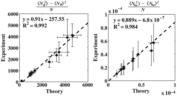
Second moment of the trajectory distribution. The x axes give the predicted second moments from the MaxCal approach, based on the known first moments. The y axes give the experimental values of the second moments. Left: Variance of 〈N_B〉; right: variance of 〈N_ba〉. The dashed lines are the best linear fits; fitting parameters are inset. Each point represents one experimentally observed trajectory. Trajectories were 30000 Δt units long, and errors were calculated for around 600 trajectories. ω_r and ω_f values ranged from 1 × 10⁻⁵ to 1 × 10⁻³.

Figure 3 compares one experimental third cumulant with the predicted value from caliber obtained from the measured first moments. The first moments are easy to measure with good accuracy from short trajectories, so one virtue of the caliber approach is that all of the higher predicted moments are noise-free compared to higher moments extracted from data: Predicted moments are dependent on first moments only, whereas data-based higher moments are contaminated by noise from every other lower moment. See the supplementary information [13] for more detail.

Fig. 3.

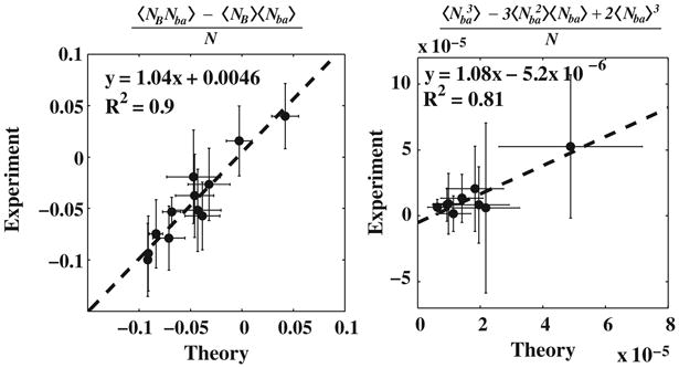
Experiments vs theory for the covariance and third cumulant. Left: One covariance quantity. Right: The third cumulant of N_ba. The dashed lines are the best linear fits; fitting parameters are inset.

Figure 3 also shows the quantity 〈N_BN_ab〉 − 〈N_B〉〈N_ab〉. These covariances, equivalent to mixed moments, give an alternative way to express reciprocal relationships resembling the Maxwell relations of thermodynamics and Onsager's reciprocal relations for dynamical processes near equilibrium. In essence, this means that one trajectory observation counts for two: Small perturbations on a trajectory are equivalent to observing covariances; thus, without performing additional experiments or recalculating Q_d, we know how the system will behave for different potential wells—just looking at the fluctuations is enough.

We can compute the ratio N_A/N_B = K. As t → ∞, this ratio simply becomes the equilibrium constant K_eq for the relative populations of the two states A and B. In the small-time limit, for this single particle, this ratio is not a single number, as it would be in a bulk equilibrium experiment; rather in single-particle cases, this has a distribution of values. Figure 4 shows these distributions for a situation in which the average is 〈N_A/N_B〉 ∼ 1. The distribution approaches a δ function as t → ∞ and thus K → K_eq. In -diffusion-related problems, small-number situations in which particles flow up concentration gradients, rather than down, have been referred to as “bad actors” [9]; the number of bad actors diminishes as trajectories get longer. We also see that simulation of the partition function matches the experimentally measured distributions of N_A/N_B. This indicates that the chosen first-moment constraints are sufficient to describe the entire trajectory space.

Fig. 4.

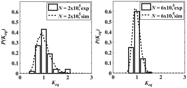
The probability distribution of N_A/N_B = K_eq as a function of time. We obtain the dashed line from Monte Carlo simulation of Q_d and corresponding columns from experimental data. The distribution of time spent in A vs B is broad for short times (left) but becomes narrower for increasing trajectory length (right). N denotes the length of each trajectory, each repeated around 100 times. As the length of trajectories increases, the equilibrium constant assumes a delta-function distribution, commensurate with equilibrium assumptions regarding chemical reactions.

In summary, we have studied a single colloidal particle undergoing a two-state process A ⇌ B with stationary rates. By measuring short trajectories, we obtain first-moment observables 〈N_bb〉, 〈N_aa〉, 〈N_ba〉, and 〈N_ab〉. The variational principle of maximum caliber is then used to predict the higher moments of the observables as well as the full probability distribution of the trajectories. Maximum caliber also gives other dynamical reciprocal quantities, resembling Maxwell-like relations. We believe that trajectory-based dynamical modeling such as this will be useful in single-molecule and few-molecule science.

References

- 1.Finzi L, Gelles J. Science. 1995;267:378. doi: 10.1126/science.7824935. [DOI] [PubMed] [Google Scholar]; van den Broek B, Vanzi F, Normanno D, Pavonea F, Wuite G. Nucleic Acids Res. 2006;34:167. doi: 10.1093/nar/gkj432. [DOI] [PMC free article] [PubMed] [Google Scholar]
- 2.Baldini G, Cannone F, Chirico G. Science. 2005;309:1096. doi: 10.1126/science.1115001. [DOI] [PubMed] [Google Scholar]; Dickson R, Cubitt A, Tsien R, Moerner W. Nature (London) 1997;388:355. doi: 10.1038/41048. [DOI] [PubMed] [Google Scholar]
- 3.Popescu G, Robert A, Howe JR, Auerbach A. Nature (London) 2004;430:790. doi: 10.1038/nature02775. [DOI] [PubMed] [Google Scholar]
- 4.Gardiner CW. Handbook of Stochastic Methods. 3rd Springer-Verlag; Heidelberg: 2004. [Google Scholar]; Brown FLH. Phys Rev Lett. 2003;90:028302. [Google Scholar]
- 5.Kramers H. Physica (Utrecht) 1940;7:284. [Google Scholar]; McCann LL, Dykmann M, Golding B. Nature (London) 1999;402:785. [Google Scholar]; Simon A, Libchaber A. Phys Rev Lett. 1992;68:3375. doi: 10.1103/PhysRevLett.68.3375. [DOI] [PubMed] [Google Scholar]; Cohen AE. Phys Rev Lett. 2005;94:118102. doi: 10.1103/PhysRevLett.94.118102. [DOI] [PubMed] [Google Scholar]
- 6.Svoboda K, Block SM. Annu Rev Biophys Biomol Struct. 1994;23:247. doi: 10.1146/annurev.bb.23.060194.001335. [DOI] [PubMed] [Google Scholar]
- 7.Lang MJ, Asbury CL, Shaevitz JW, Block SM. Biophys J. 2002;83:491. doi: 10.1016/S0006-3495(02)75185-0. [DOI] [PMC free article] [PubMed] [Google Scholar]
- 8.Jaynes ET. In: Complex Systems: Operational Approaches in Neurobiology, Physics and Computers. Haken H, editor. Springer-Verlag; Berlin: 1985. p. 254. [Google Scholar]; Jaynes ET. In: The Maximum Entropy Formalism. Levine R, Tribus M, editors. MIT; Cambridge, MA: 1979. p. 15. [Google Scholar]; Jaynes ET. Annu Rev Phys Chem. 1980;31:579. [Google Scholar]; Grandy W. Phys Rep. 1980;62:175. [Google Scholar]
- 9.Seitaridou E, Inamdar MM, Ghosh K, Dill KA, Phillips R. J Phys Chem B. 2007;111:2288. doi: 10.1021/jp067036j. [DOI] [PMC free article] [PubMed] [Google Scholar]; Ghosh K, Dill K, Inamdar MM, Seitaridou E, Phillips R. Am J Phys. 2006;74:123. doi: 10.1119/1.2142789. [DOI] [PMC free article] [PubMed] [Google Scholar]
- 10.Stock G, Ghosh K, Dill KA. J Chem Phys. 2008;128:194102. doi: 10.1063/1.2918345. [DOI] [PMC free article] [PubMed] [Google Scholar]
- 11.Wu D. unpublished. [Google Scholar]
- 12.Dill KA, Bromberg S. Molecular Driving Forces: Statistical Thermodynamics in Chemistry and Biology. Garland Science; New York: 2003. [Google Scholar]
- 13.See EPAPS Document No. E-PRLTAO-103-018933 for a description of our efforts to reduce the standard error of Figs. 2 and 3 by checking the MaxCal algorithm against Brownian dynamics generated trajectories and a demonstration of the convergence properties of predicting higher order moments of trajectories using MaxCal by plotting the theoretical predictions against simulated moments as a function of trajectory length; in short, we show that the MaxCal predictions converge to the true value of the higher order moments as fast or faster than simulated ones. For more informationon EPAPS, see http://www.aip.org/pubservs/epaps.html.
Associated Data
This section collects any data citations, data availability statements, or supplementary materials included in this article.