MOIL-opt: Energy-Conserving Molecular Dynamics on a GPU/CPU system

Abstract

We report an optimized version of the molecular dynamics program MOIL that runs on a shared memory system with OpenMP and exploits the power of a Graphics Processing Unit (GPU). The model is of heterogeneous computing system on a single node with several cores sharing the same memory and a GPU. This is a typical laboratory tool, which provides excellent performance at minimal cost. Besides performance, emphasis is made on accuracy and stability of the algorithm probed by energy conservation for explicit-solvent atomically-detailed-models. Especially for long simulations energy conservation is critical due to the phenomenon known as “energy drift” in which energy errors accumulate linearly as a function of simulation time. To achieve long time dynamics with acceptable accuracy the drift must be particularly small. We identify several means of controlling long-time numerical accuracy while maintaining excellent speedup. To maintain a high level of energy conservation SHAKE and the Ewald reciprocal summation are run in double precision. Double precision summation of real-space non-bonded interactions improves energy conservation. In our best option, the energy drift using 1fs for a time step while constraining the distances of all bonds, is undetectable in 10ns simulation of solvated DHFR (Dihydrofolate reductase). Faster options, shaking only bonds with hydrogen atoms, are also very well behaved and have drifts of less than 1kcal/mol per nanosecond of the same system. CPU/GPU implementations require changes in programming models. We consider the use of a list of neighbors and quadratic versus linear interpolation in lookup tables of different sizes. Quadratic interpolation with a smaller number of grid points is faster than linear lookup tables (with finer representation) without loss of accuracy. Atomic neighbor lists were found most efficient. Typical speedups are about a factor of 10 compared to a single-core single-precision code.

I. Introduction

Molecular dynamics and its computational challenges

Molecular Dynamics (MD) simulations have become a vital laboratory tool for investigations of molecular processes in fundamental statistical mechanics, material science, and biophysics. Molecular Dynamics trajectories provide significant insights into mechanisms, enable the rational design of new materials, and test new analytical theories by exact numerical calculations. In the present manuscript we restrict the discussion to algorithms that follow the classical equations of motions, conserve energy, and therefore enable basic study of dynamic phenomena. Molecular trajectories are computed in small time steps using initial value solvers that propagate the solution in time steps. The existence of fast motions at the atomic scale (e.g. molecular vibrations) necessitates the use of small time steps (femtoseconds ∼10^-15s) that are much shorter than times of many processes of interests. For example, folding (milliseconds), and conformational transitions of proteins (microseconds) occur on time scales much longer than femtoseconds. Billions of steps (and more) must be computed in order to reach relevant times. This significant time scale gap (twelve orders of magnitudes from femtoseconds to milliseconds) motivates research into the extension of time scales in atomically detailed simulations.

The search for longer simulation times in atomically-detailed, solvent-explicit models, is theoretical, numerical, and computational. On the theory side alternative formulations of classical mechanics and statistical mechanics were proposed, such as the use of boundary value formulation with large time steps ¹, sampling of rare (but rapid) trajectories ², and the patching of trajectory fragments ³. These theories aimed at reducing the number of time steps required to obtain a desired result. For specific systems, or with acceptance of physically-motivated approximations, the reduction in the overall time steps required can easily reach billions⁴. On the numerical side, algorithms were introduced for more rapid calculations of the forces (e.g. PME⁵), and for the use of multiple time steps (e.g. RESPA⁶) The use of a small time step for fast motions and a larger time step for slower motion allows for further efficiency gains. While the impact of the theory on the computational efforts was larger than that of numerical analysis (multiple time steps as such did not increase efficiency by more than a factor of two) there remains the interest in conducting simulations without approximations or theoretical assumptions on the system type. The third approach to long time scales is of computational techniques attached to advances in hardware. This approach dominates the advances in straightforward simulations (no physical assumptions or constraints on the system type are assumed) in the last 10 years.

Faster computational systems have the promise of speeding up simulations times considerably. Indeed a special purpose computing machine, the Anton⁷, produced trajectories at the millisecond time scales. Cost, however, is an issue, and as a laboratory tool Anton is out of reach of many research groups. Besides the development of a special purpose machine for MD, in the last 10 years we have seen significant advances in parallel hardware and software architectures. While the speed of individual computing elements did not increase significantly, parallelism of different varieties is now accessible at multiple levels. Cores, or basic computing elements, are available in distributed and shared memory configurations, complicating software development but also offering new opportunities. Another new hardware development of considerable interest is the use of graphics processing units (GPU) originally designed for the game industry. The massive parallelism of the GPU attracted the attention of computational scientists, promoting the development of the high level programming language CUDA. A number of important scientific applications were ported to the GPU platform ^{7b, 8}. For the cost (mid-to-high end GPU cards can be found for ∼$200) graphics processing units provide unmatched computing power. The complete computing node that was used and benchmarked in this work: an MSI-G65 board with 8GB 1333MHZ RAM, a Phenom™ IIX4 965 3.4GHZ processor, a 1 TB hard drive and a single GTX480, costs ∼$1,200. This makes it possible for applications that exploit it to run at high performance speeds accessible to a broad range of investigators.

On the other hand exploiting the promise of the GPU for Molecular Dynamics applications is not a trivial task and requires a departure from legacy codes, the use of new programming models, and learning to code with new constraints on memory sizes and memory hierarchy. It is therefore not surprising that general-purpose Molecular Dynamics software packages with modeling of explicit solvent were slow to emerge for the GPU^{7b, 8}. In some cases the performance was not satisfactory and in others energy conservation (essential for calculations in microcanonical ensemble) was compromised.

There are two common models for computational chemistry. The first uses high-end supercomputers and the second employs laboratory tools such as PC and local computing clusters. Both approaches were found to be very useful throughout the years and are employed (frequently simultaneously) in many laboratories. Typically a calculation that requires a lot of resources for a short period of time is better run at national centers while calculations that require long running periods are better run at laboratory resources. For example, solving hundreds of millions of coupled equations is better done using massive parallelism on hundreds of cores ⁹, while running a large number of straightforward and short trajectories to obtain statistics for thermodynamic and kinetic averages ⁴ is more effectively conducted on computer clusters, common to individual laboratories.

What are the challenges in implementing codes on a combination of CPU/GPU beyond the need to learn to use a new hardware platform, its limitations, and compilers?

The first is the realization that the GPU is not optimal for everything. Though some attempts were made to put a whole MD code on a GPU, the performance is lacking for complex systems that include a diverse set of interactions (e.g. covalent and non-covalent components), or that require double precision accuracy. Memory access is important and can be a bottleneck in the calculations. If the system is simple and uniform (e.g. Lennard Jones fluids ¹⁰), then it makes sense to implement the entire MD code on the GPU. For other cases it is not obvious.

It is therefore suggestive to use the GPU for the parts that it is best at, massive parallel execution of simple and minimal instruction sets and asynchronously use the cores at the CPU for complex calculations, or calculations that require double precision. Practice has shown that the communication between the GPU and the CPU is not a bottleneck with systems of sufficient complexity.

The second challenge is of load balancing between the CPU and GPU. Ideally we wish the CPU and the GPU to spend the same time on their assigned load. This is however a complex task and so far we have not been able to achieve it in full. At present our code still has bottlenecks in which the GPU is waiting for the CPU to complete its task. Further optimization of the load is a topic for future studies.

Third the mixture of computer language, compilers and libraries (OpenMP, CUDA, C and FORTRAN) makes the code highly complex. It is difficult to maintain and it is sensitive to hardware configurations. Relatively minor changes in hardware, operating system, or compiler versions can induce non-trivial code and compilation changes. Sustaining MD programs is simpler for those who remain in the CPU world. For the program reported in this manuscript we offer binary executables that run on a variety of Intel/AMD multi core CPU and Nvidia CUDA capable GPU equipped systems with the appropriate drivers installed http://clsb.ices.utexas.edu/prebuilt/. We also provide a source code, but advise the user that getting CPU/GPU code to compile and produce an executable file is more difficult than typing “make” and <enter> because third party hardware and software drivers/libraries (not provided by us) are involved.

Despite the above difficulties significant speed-ups were obtained on a single heterogeneous node (multi-cores, one GPU) for a broad range of Molecular Dynamics applications. The factors are ∼10 compared to running on a single core with a single precision code. This makes the investments in solving the above challenges a worthwhile exercise.

In the present manuscript we therefore describe the implementation of a molecular dynamics module of the modeling package MOIL¹¹ on such a single-node heterogeneous-system. MOIL is a suite of programs that are written in FORTRAN and span a wide range of modeling tasks. Some of its options include energy minimization, reaction path calculations¹², rate calculations by Milestoning^3b, Molecular Dynamics and more (see http://clsb.ices.utexas.edu/prebuilt/MOIL.pdf for a comprehensive description). To facilitate the GPU, code was written in CUDA to compute the non-bonded list and real space non-bonded interactions on the GPU. The overall Molecular Dynamics driver was written in C and so was the Verlet (or RESPA) integrators. The rest of the calculations that are performed on the CPU remained in FORTRAN. Code on the CPU that influences the overall performance, the PME reciprocal summation, SHAKE¹³ of water molecules, and SHAKE of bonds that contain hydrogen atoms, was parallelized using OpenMP. We discuss below the choices made, speed of calculations and energy conservation.

Energy conservation is especially important for calculations that determine rate and time scales from microscopic theories and modeling. While stochastic dynamics was proposed to overcome problems with energy conservation, these corrections are questionable for dynamics. For example, the use of the Langevin equation with a phenomenological friction significantly impacts the rate. At the high friction limit the rate is inversely proportional to the friction, making it impossible to determine the rate constant from microscopic parameters only.

II. Implementation

At an abstract level Molecular Dynamics algorithms typically have the following structure:

Do while [current number of integration steps < desired number of integration steps]

1. Compute forces (bonded, real space non-bonded, reciprocal space non-bonded)

2. Increase total time by a time step.

3. Compute a displacement in coordinate space

4. Adjust coordinates to satisfy constraints

5. Compute velocity displacements

6. Adjust velocities to satisfy constraints

7. Output: intermediate coordinates and velocities, energies, etc.

End while

For typical systems the most time consuming part is the calculation of the forces, and the most expensive component of the force calculations is the computation of the non-bonded interactions (Supporting Information D). We restrict our optimization to simulations with explicit solvation and periodic boundary conditions as the most appropriate for atomically-detailed simulations of molecular kinetics (without the explicit inclusion of quantum effects). Molecular kinetics is a focus of research in our group. We split the calculation of electrostatic to real and reciprocal space using an Ewald summation scheme. Only the real part of the non-bonded calculation is performed on the GPU. The rest of the calculations are performed on the CPU using OpenMP to exploit the multi-core shared memory system. Below we provide more details on the implementation.

II.1 memory concerns

To appreciate the complexity of GPU programming it is necessary to consider its memory architecture.

The GPU has a reasonably large global memory (1.5GB in the machine we benchmarked on), which is relatively slow. Fetching data directly from the global memory to the GPU cores is costly. Therefore, programming models attempt to maximize the use of intermediate and faster memories as bridges between the global memory and the executing threads.

For a more detailed discussion on CUDA basics we refer to previous work^{7b, 10, 14}. Briefly, the fastest memories available in CUDA are the thread local registers, shared memory and constant memory. Shared memory is available only throughout a single thread block. Constant memory is available to all threads on the GPU but extremely limited in size (64 kb total) and read only. There are few registers available per thread (∼32) and they must be used carefully. For example, during the calculation of the non-bonded interactions between atom i and its neighbors j, thread local registers keep the coordinates of atom i, the index of this atom and temporarily store the pair parameters for Lennard Jones interactions A_ij and B_ij, and the product of the atomic charges q_iq_j during the force calculation. The thread computes and retains (also in thread local registers) the three components of the forces operating on the i atom: f_xf_yf_z. There is little space to do more on a single thread and therefore calculations on an individual thread are conducted for one atom pair at a time (loop unrolling has little or no benefit).

The next best resource after registers, constant and shared memory are caches on global RAM. Depending on the system at hand, shared memory can be replaced by texture memory cache or L1 cache available on the global memory of newer chips. However, as a consistent feature of GPU hardware options, old and new, the shared memory suggests itself as an indispensible bridge between the global and register memory and we use it extensively. For example we place lookup table for non-bonded interactions (interpolated quadratically between the table points) on the shared memory.

II.2 Particle Meshed Ewald

Other codes port the reciprocal sum of the Particle Meshed Ewald (rsPME) calculations to the GPU¹⁵. However, in our hands the rsPME calculations in single precision were not accurate enough to avoid significant energy drift. For the purpose of the present manuscript we define “significant energy drift” as an energy variation that exceeds 1 kcal/mole in a nanosecond simulation of DHFR, Dihydrofolate reductase. Since empirically the drift is linear in time, one kcal/mole drift in a nanosecond is about 1,000 kcal/mole in a microsecond, enough energy to break several chemical bonds. While the excess energy is (of course) distributed in many degrees of freedom it is likely to influence significantly the results. The kinetic energy of the system is about 15,000 kcal/mole at room temperature and 1,000 kcal/mole is ∼6.7% of the total, or changing the temperature by ∼20°K.

In a periodic box of water, DHFR has become a standard benchmark for Molecular Dynamics codes (for example http://ambermd.org/amber8.bench2.html). The complexity of the rsPME calculations is considerable. About 1/3 of the total computation time in a serial code is spent in rsPME calculation, if the Verlet algorithm is used.Supporting Information D includes a profile of a serial MOIL run. Note, however, that the profile reported used RESPA⁶ in which the reciprocal sum is computed every four steps, see below. We took the following steps to speed rsPME up: (i) It was parallelized using OpenMP, and (ii) It is computed less frequently using multiple time steps, and (iii) It is computed asynchronously on the CPU while the GPU is working on real space summation. We use reversible multiple time stepping algorithm (RESPA⁶) to integrate the equation of motion where we designate the reciprocal sum as the “slow” force. The forces are split into two, a fast varying component F^f and a slow varying force F^s. Bond constraints (SHAKE ^13a) and matrix SHAKE for water molecules (MSHAKE ^13b) are included in the inner loop of the algorithm.

Studies by¹⁶ illustrate that the reciprocal sum has a fast force component, and a better behaving algorithm can be designed that includes a combination of real space and reciprocal space as the slowly varying force. A more elaborate and accurate force splitting has been described in which fast components of the pair interactions are removed from the reciprocal space Ewald sum. The authors reported an enhance in the stability of the algorithm to an outer time step of 6 fs although the level of stability depended on the choice of the parameters for a switching function used to smooth the potential energy near the cutoffs. In our hand (and also in the paper ¹⁶, figure 3) a large time step size of four femtoseconds for the integration of the reciprocal sum and one femtosecond for the rest of the forces was stable and did not show energy drift. We therefore consider only the reciprocal force as slow. Use of this algorithmic variation in our code and its effect on stability and computation speed will be explored in the future. In the context of heterogeneous GPU/CPU computing, mixing real space and reciprocal space increases the computational complexity significantly.

Figure 3.

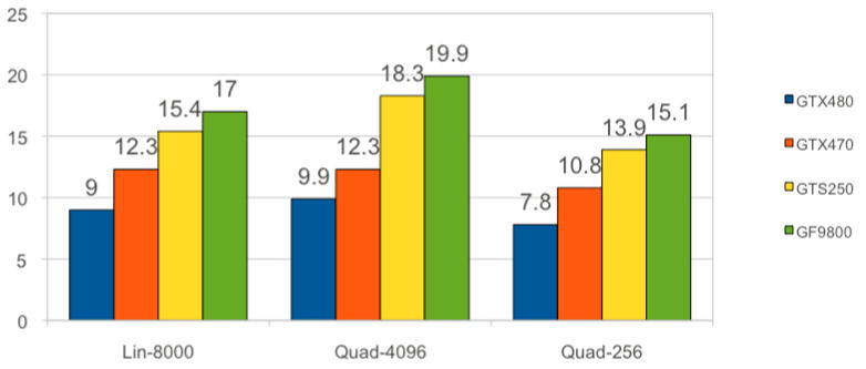
Timing in ms/step for calculations of non-bonded interactions for different GPUs and different options for lookup tables. The rest of the calculations in the GPU presented in this paper were done on the GTX480. The numbers below include force calculations and communication between the GPU and the CPU. Quad-256 is a table with quadratic interpolation of 256 entries that resides in the shared memory. It is the fastest option and retains acceptable accuracy (Table 2). Quad-4096 is a quadratic table with 4096 entries, which is our most accurate option, and only moderately more expensive than the other options. It is too large to fit in the shared memory and resides mostly in the texture memory. Lin-8000 is a linear interpolation scheme that resides mostly in the texture memory and offers no advantage, accuracy or speed-wise, compared to Quad-256. Coalescing the data is critical. If the data of the non-bonded list matrix M_ij is not coalesced then running on GTX480 the Quad-4096 option increases the time from 9.9 to 16.5ms

The calculations of the reciprocal sum were further accelerated by parallelization of the basic FFT algorithm, and of the generation of the required charge grid using OpenMP The parallelization was performed directly on the public domain PME code of Darden ⁵. No changes to the basic algorithm were made. We use cubic polynomial for grid interpolation and tolerance of error of 10^-9 for double precision calculations. Parallelization of the non-FFT routines was done trivially by splitting up the loops between cores (e.g. in the routines fill-charge-grid and scalar-sum). The x, y, z components were parallelized with synchronization after the completion of each Cartesian direction. A recent suggestion by Schneiders et al. ¹⁷ for parallelization of convolutions can improve the performance of the code. However, the present program is functional and efficient enough to remove the reciprocal sum as a major hurdle of the calculation. The bottleneck is still the calculation of real space non-bonded interactions.

II.3 Non-bonded list

Besides the concrete and specific implementation, perhaps the first question to ask is do we need a non-bonded list at all? In principle there are few options: (i) Do not use list, compute all against all, (ii) use a space list based on grid partitioning, (iii) use a list based on chemical grouping, and (iv) used lists based on atoms. All of these ideas were used extensively in molecular simulations in the past but they were reconsidered and found new ground in GPU implementations.

Option (i) was used for illustration purposes on systems with non-uniform particle densities. For example, protein molecules simulated with implicit solvent does not fit an exact grid, and have a relatively small number of interactions. An implementation on the GPU for all-against-all interactions can provide good-looking benchmarks (results not shown). However, most MOIL applications aim at studies of explicit solvent systems in the NVE ensemble.

Option (ii) is used by a number of groups ^{7b, 8, 10, 14}. We consider periodic system of approximately uniform density. The space is partitioned to boxes, and individual particles are placed in a box list in an operation of complexity N¹⁸. For example if the grid sizes along the x,y,z directions are g_x,g_y,g_z respectively, a particle with coordinate x,y,z (where the origin of coordinates is such that x,y,z ≥ 0 for all the particles in the system) is placed in a box index (i,j,k)= (⌊.x/g_x⌋, ⌊y/g_y⌋,⌊z/g_z⌋) where the counting starts from zero. Box neighbors are, of course, known. For each atom there are 27 neighboring boxes including its own box. Based on box neighbor list the interactions between atoms of nearby boxes and of the self box are computed. The advantage of this representation is that no atomic list is produced. Atomic list tends to be long and expensive in terms of storage memory. It cannot be placed directly in the registers or in the shared memory, while box-lists can reside in the shared memory. The box lists are particularly convenient for large systems, and we use them in cases that exceed 100,000 particles. A disadvantage is that box-based lists are not precise. The neighbors are not distributed spherically around each atom. The number of atom pairs is larger and requires more computational resources. Another disadvantage is that the force kernel for a box list is complex and that hinders the use of accurate quadratic lookup tables because the limit of 32 registers per thread will be exceeded. This is since we will not be able to compactly and efficiently transfer to the thread one atom-pair at a time. Yet another disadvantage is that the exclusions are not explicitly removed at the level of the lists. Therefore, when the force calculations are performed, a logical check is performed, and the excluded interactions are multiplied by zero.

Option (iii) of chemical grouping replaces the box-based list by a list of neighboring chemical groups. It was used in MOIL¹¹ for decades. An issue with parallelization is of load-balancing which was addressed and discussed in ^13b. In ¹⁹ it was proposed to collect atoms in groups of 32 for GPU applications. This procedure provides a uniform density and fits well the GPU specifications. Nevertheless, collections of this type requires periodic calculations of groups for diffusive particles (such as water molecules), and the scaling of these calculations as a function of the distances between groups is ∼N², which is unfavorable for large systems.

Option (iv), which we adopt for systems smaller than 100,000 atoms, is hierarchical. We generate a box-based list and we use that list to generate the atomic list (a list of atoms with a distance equal or smaller than a cutoff distance from the central atom i). The advantages of the atomic list are that the exclusions are taken care of during the generation of the list and that the atomic list is precise and spherical around each atom. The atomic list is generated according to two cutoffs in which the upper cutoff provides the actual list and is used as a buffer between updates of the lists. Pair calculations are performed only between pairs that are closer than the lower cutoff distance. This means that the calculations of forces are as efficient as possible. A disadvantage is the size of the list. Following Anderson¹⁰, the list is stored as a matrix in the global memory N_ij, where the index i is running over the atom number and the index j over its neighbors. It is possible to make the list more efficient by using a pointer vector, P, of the length of the number of atoms, and the actual list N. P(i) points to the last neighbor of i in N^13b. Hence the neighbors of i are listed between N(i-1)+1 to N(i). Since the density in molecular biophysics simulations is quite uniform, the number of neighbors per atom is rarely changing by more than 10 percent, and hence both representations are of comparable complexity. For a typical real space cutoff every atom has about 500 neighbors.

For the generation of the list for atom i we load the index of atom i, its coordinates, and the non-bonded parameters, A_i, B_i, and q_i, to the registers. We load from the global memory to the shared memory the coordinates and the corresponding parameters of a box neighbor to i. The individual threads can access rapidly the shared memory and produce the atomic lists of all pairs with distances lower than the distance cutoff. They also produce the corresponding products A_ij ≡ A_iA_j, B_ij ≡ B_iB_j, and q_iq_j ≡ q_ij. The preliminary calculations of the products provide more benefit than saving a few multiplications for a pair of atoms. These products are stored together in the global memory and can be accessed when needed for the force calculations in coalesced and efficient way. The GPU has a particularly efficient memory operation (float4 array) in which four floating-point numbers are transferred between memory types in one chunk. We transfer in a float4 chunk, the atom index i, its Lennard Jones parameters for the pair, A_ijB_ij, and its charge product q_ij. Exclusion of bonded atoms is accomplished by chemical sorting of the atoms to begin with. Most of the bonded atoms are within 32 positions of the general atom index, (with the exception of S-S bonds, prosthetic groups like heme, etc.), allowing the storage of an exclusion decision in a single bit, +1 means exclusion. The basic algorithm for exclusion is the same as reported in ^7b, however the retention and preliminary calculations of the pair parameter is new and adds significantly to the performance. For the rare (if any) excluded pairs, that are out of the 32 range, the corresponding force is subtracted in a separate kernel.

II.4 Non-bonded forces

We describe in detail the calculation of the forces, utilizing an atomic list. Similarly to the calculation of the list a thread is associated with a single atom i. We store and accumulate in registers the forces that operate on this atom and we loop over the neighboring atoms with their prepared coefficients (see II.3 Non-bonded list). The coefficients are copied in coalesced and efficient way from the global memory in float4 arrays. Coordinates of neighbors need to be read from global memory and these reads are not coalesced. This however does not lead to significant performance lag, probably because the large amount of computations that follow cover up some of the memory fetch time and the coordinate fetch is at least partially cached. Similar performances are obtained if the coordinates are read from texture cache or directly from the global memory of newer chips which feature an adjustable L1 cache on global RAM. In the latter case we adjust the L1 cache to its maximum size of 48 KB.

Once all the parameters are in, the square of the distance between a pair of particles is computed on each thread. With the square of the distance at hand, explicit and direct calculations of the electrostatic and van der Waals interactions can be performed. A useful trick, which is employed for a long time by now in MD codes, is the use of lookup tables to present complex functions of the square of the distance (e.g. the error function that is used in Ewald sums). The lookup table provides the value of the function on a grid. For a more precise value an interpolation between the grid points is required. If the table is dense (say, 10,000 grid points) the interpolation can be simple (linear) as is done in ^7b, fetching the value from the texture memory. The texture memory is however relatively slow even when 100% cached and it is desirable to place the table in shared or constant memory. This is possible only for small tables. We successfully used exceptionally short tables with 256 or 512 entries interpolated with quadratic lookup (see Supporting Information A and C). The accuracy of the forces is sufficient for good energy conservation and memory access is no longer a bottleneck. The calculations of real space PME electrostatic are complex and justify the use of a table and memory fetches. We found out however that the Lennard Jones interactions are faster computed directly instead of looking up for values in interpolated tables. Hence, the Lennard Jones calculations are computed directly on the thread.

Note that we do not take advantage of the symmetry in interactions between particles, i.e. we compute the interaction between the pair of atoms (i, j) twice. We compute it once with atom i at the center, and a second time with atom j at the center. This is clearly inefficient. However, minimizing communication is more important here than saving floating point operations. Overall re-computing these interactions makes more sense here as is also done by others ^{7b, 8, 10}.

Pseudo codes for the generation of the non-bonded lists and the calculations of the forces can be found in Supporting Information B and C respectively.

II.5 Use of OpenMP

Computing environments change rapidly. A trend of the last few years is a significant increase in the number of cores on a CPU and the creation of powerful, and shared memory machines. The recent announcement by Intel of a chip with 50 cores http://www.electronista.com/articles/10/05/31/intel.knights.corner.targets.highly.parallel.pcs/ is a particularly significant step making shared memory programming a mainstream approach. While a distributed computing approach can provide a significantly larger number of cores, the ease and efficiency of a shared memory implementation where communication speed is no longer an issue are very attractive. Shared memory machines are also more likely to be the machine of choice for a laboratory instrument. We therefore decided to base our new implementation of MOIL on a model of shared memory CPU with the relatively low-cost option of a GPU. Most molecular dynamics programs (including an earlier version of MOIL ^{11, 13b}) were built for distributed computing environment and their parallelization is based on Message Passage Interface (MPI, http://www.mcs.anl.gov/research/projects/mpi/). Here we are starting fresh and base our programming model on OpenMP (http://openmp.org/wp/), which is a library designed for shared memory systems. We parallelized the reciprocal sum calculations of the PME (see section II.2), the Verlet algorithm and MSHAKE algorithm (matrix SHAKE ^13b) that constrained the geometries of water molecules. While a parallel algorithm for general SHAKE constraints was designed in the context of the MOIL program ^13b, at present this algorithm is not available in OpenMP and this is the topic of future work. Similarly to other groups we parallelize SHAKE constraints for bonds that contain hydrogen atoms. We call this variant SHKL (SHAKE light). These bonds are separated into independent blocks of constraints and can be trivially parallelized on the multiple cores by OpenMP. We also comment that if SHAKE of all bonds is calculated (at present only serially) then the energy conservation with 1fs time step and room temperature simulation of solvated DHFR is excellent. There is no detectable drift when we use 4096-entries quadratic-interpolation table of the real-space electrostatic interactions. However, the cost of serial calculations of SHAKE is high and it reduces the overall speed of calculations by about 30%.

In Figure 2 we sketch the scaling of our OpenMP calculations of DHFR on a single node. An unusual observation is that the scaling of SHKL is better than the number of processors. This result is obtained since the convergence decision is made locally in each core. It is not necessary to wait for convergence for the slowest relaxing bond in the list (like is done in a serial calculation) but instead we can decide on the convergence based on the local bonds assigned to a core. These bonds are decoupled from the rest. The figure also shows that further optimization of the PME code is needed and is a topic for future work.

Figure 2.

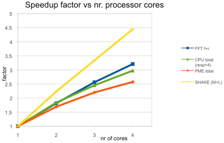
Efficiency of parallelization of components of the Molecular Dynamics algorithms computed with OpenMP. The yellow line is the scaling of the SHAKE algorithm. The red line is the complete PME reciprocal sum. The blue line is only the Fast Fourier Transform of the PME reciprocal sum (f is forward and r reverse), and the green line is the scaling of the overall OpenMP code. See text for more details.

We did not try to design an algorithm where all the calculations are performed on the GPU, (or did not try to maximize the role of the GPU in executing the calculations) due to concerns about accuracy and single precision. Calculations on GPU are efficient if done in single precision. Recent GPU architecture allows calculations in double precision but the penalty in performance is high. Besides the final summation of the forces, using double precision for non-bonded force calculations on the GPU is not practical at present. The reason is not only that double precision operations are slower on the GPU, but also that the memory is limited. Doubling the data needed means that we will require registers that are simply not available and the code will be unacceptably slow. Our requirement for energy conservation mandated that the reciprocal sum is computed in double precision and therefore we prefer to execute it on the CPU. Further discussions about energy conservation can be found in section III.6.2.

III. Results

All tests run (unless specifically stated otherwise) on MSI-G65 8GB 1333MHZ RAM Phenom™ IIX4 965 3.4GHZ with a single GTX480. We describe below applications of MOIL-opt to moderately sized systems. These systems are more likely to be investigated in a laboratory setting which is our target. Since they are relatively small, they are less likely to produce impressive benchmarks. However, as we illustrate below, we are getting consistently good performance with no compromises in the numerical accuracy of the simulations. We discuss typical inputs, conditions, and timing. In the calculations below the tolerance for relative errors of constraints was always 10^-12. The recommended choice for the reciprocal sum calculations on the CPU is to be conducted in double precision and allowed relative errors were 10^-9. We discuss in III.6.2 Energy conservation the impact of a single precision calculation. As a reference for performance we compared these simulations (GPU code with mixed single/double precision accuracy) to simulations conducted on one CPU core in single precision. While critical accuracy can be lost in single precision calculations, these comparisons provide a good measure and a lower bound of the speedup obtained in the heterogeneous environment of the GPU/CPU. The other alternative we have in MOIL (calculations on one core in double precision) is significantly slower. The new lookup tables built for the GPU/CPU code are more accurate than the tables of the double precision, older version of MOIL¹¹. As a result, the energy conservation at long time scales is actually better in the GPU/CPU version than the older double precision version. Sections III. 1 to III.5 focus on the performance of MOIL-opt for different molecular systems.

A quick summary of our observations is in the table below:

III.1 DHFR

We report a simulation in a periodic box of aqueous solution of size 62.23×62.23×62.23 ų with the use of PME for long-range electrostatics. Real space cutoff distances define two layers (to create a buffer during the calculations of the forces) which are of 8.5Å and 8.8Å respectively. Forces between particles in the list that are separated by distances larger than the lower cutoff are not computed. The total number of boxes used in the generation of the non-bonded list was 7³.

The non-bonded list was updated every 7 steps. The time step was 1fs and the PME mesh was of 64³ points. The number of particles was 23,536. The force field was OPLS-AA ²⁰ with the TIP3P water model ²¹. A quadratic lookup table for electrostatic interactions with 256 entries was used. Lennard-Jones interactions were computed explicitly. Water molecules were kept rigid with MSHAKE (Matrix SHAKE) and all bonds that include hydrogen atoms were constrained as well. All components of the program run in parallel, either on the GPU or on (at most) four cores of the CPU. Direct, constant energy simulations (NVE ensemble) were conducted. The RESPA algorithm was used with a 4fs time step for integrating the PME reciprocal forces and 1 femtosecond for the rest of the interactions. Examining the exclusion list, only three particle pairs were beyond the 32 range for this system. The interactions of these pairs were explicitly subtracted on the GPU from the forces of these particles. The calculations on the CPU and the GPU are conducted (to the extent possible) asynchronously. At the time that the non-bonded interactions are computed on the GPU, the CPU is busy computing the reciprocal sum and the covalent interactions. It should be noted that overall the GPU is faster. It typically waits for the CPU cores we used for the OpenMP parallelized calculations to complete their tasks. Use of more cores in the future can tilt this balance. However, more than speed, our concern with the distribution of the work between the GPU and the CPU is of accuracy and energy conservation.

The run described above with a single thread on the CPU generates 2.27 nanoseconds a day, with two threads 3.42ns/day, three threads 4.07ns/day, and four threads 4.5ns/day. The CPU scaling leaves room for improvement, but the use of multiple cores is still useful. Times for different components in the calculations (per step) for a single core are as follows: Real space non-bonded interactions (GPU):7.80ms, Covalent interactions (CPU): 1.31ms, Reciprocal sum (computed every four steps on the CPU): 18.5ms, Generation of non-bonded list (GPU): 1.24ms, SHAKE (CPU): 10.98ms, Verlet integration (CPU): 0.50ms. Note the significant computation time for the PME and SHAKE calculations (that can benefit from more cores).

Using four threads the timing of the CPU changes as follows: Covalent interactions (not parallel, since the overall contribution is small): 1.31ms, Reciprocal sum: 7.19ms, SHAKE: 2.47ms, Verlet 0.55ms. It is clear that adding more cores and bringing the calculation on the CPU to be at par with the timing of the GPU can speed up the calculations further.

A comparable single precision calculation on one core (no GPU) generates 421 picoseconds per day. Hence the speed up we see for this system is about a factor of 10, while the accuracy is higher on the mixed CPU/GPU system.

The DHFR system is a standard benchmark in the field. However, many other applications different in sizes and complexities are also investigated in numerous laboratories and it is important to appreciate the flexibility of the code in addressing different systems. The examples below also illustrate the range of changes in the system parameters that we can do while still retaining excellent energy conservation.

III.2 Membrane system

Consider a bilayer membrane that consists of 128 DOPC phospholipids with 38,802 particles including SPC water molecules ²² and sodium chloride ions. Besides the water model, in this case the force field was OPLS-UA²³. The system is embedded in a periodic box of 65×65×120 ų. The simulation runs at room temperature with a time step of 1fs and the NVE ensemble. The cutoff distances were 9.8Å and 9.0Å. Periodic boundary conditions and PME for electrostatic calculations are used. The number of grid points was 64³ for the mesh. There were no excluded atoms beyond the 32 range, ensuring efficient calculations of the exclusion lists and the real space non-bonded interactions. A look up table of 256 grid values with quadratic interpolation was used to compute real-space electrostatic interactions. Water molecules were MSHAKEd. Simulating this system on four threads produce 3.18ns/day. By far the most expensive calculation is the real space non-bonded interactions (total of 16.40ms/step). The calculation of the neighbor list requires 2.16ms/step. Calculations conducted on the CPU with four threads include: Covalent forces (1.93ms/step), Reciprocal sum (8.38ms/step), SHAKE (1.76ms/step).

In this particular case it is the GPU that is slower and completing its task after the CPU. Additional savings in computer time are obtained from the asynchronous calculations, about 4ms/step or 14.9% of the total time.

On one core, using a single precision calculation, the performance is of 209 picoseconds a day. The GPU/CPU system speed up these calculations by about a factor of 15 to 3.18ns per day.

III.3 Twenty amino acid solvated helix (LKKLGKKLLKKLLKKGLKKL) (Peptide I)

The motivation of studying this peptide was reference²⁴. We collaborate with the authors that helped us build the initial system. Both MSHAKE for water molecules and SHKL were used in parallel on the CPU. The temperature was 300K and the cutoff distances were 9.8Å and 9.0Å. The non-bonded list was updated each 8 steps. The calculations were conducted in the NVE ensemble in a box size 59×9×9ų with a grid of 64³ for the reciprocal space calculations. We also used the most accurate interpolation option for real space electrostatic calculation (quadratic interpolation with a table of 4096 entries). This explains why the performance on the GPU is not so impressive in this case. The time step was 1fs The total number of particles was 20,235. The calculations on the GPU took 12.20ms/step for non-bonded interactions and 1.12ms/step for the generation of the list. The reciprocal summation was the most expensive calculation conducted on the CPU (with three threads): 8.32ms/step, followed by SHAKE (1.62ms/step), the Verlet integration (no RESPA was used in the present example) 0.40ms/step, and covalent interactions (0.23ms/step). The overall speed of this simulation of a peptide solvated in a large box of water was 3.7ns/day

The single precision run on one core in this case produced 426 picoseconds per day. This is about a factor of 9 slower than the CPU/GPU system.

III.4 Tryptophan zipper (SWTWEGNKWSWK)

In this solvated system we have a total of 5,847 particles, with 1875 TIP3P water molecules. The box size was 40×40×40ų and only 16³ mesh points were used for the reciprocal sum. The time step was 2fs and no RESPA integration was used. MSHAKE and SHKL were used. The cutoff distances were 9.0 and 8.5 respectively, and the non-bonded list was updated each 7 steps. The system with four OpenMP threads produces 45ns/day. Interestingly 35.5% of the CPU/GPU calculations are conducted asynchronously. Real space non-bonded interactions require 2.2ms/step (GPU), and generating the non-bonded list, 0.50ms/step (GPU). On the CPU we have the covalent forces (0.14ms/step), the reciprocal sum (1.73ms/step), SHAKE (0.41ms/step), and Verlet integration (0.19ms/step).

The one core single precision calculation yielded 3.8ns per day in this case with the same input (2fs time step) indicating a factor of ∼12 speedup.

III.5 Solvated cyclic peptide (CA₄C) (Peptide II)

This is a particularly small system of only 2,690 atoms (including 882 water molecules). The system is embedded in a box of 30.1³Å³ with only 16³ grid points for the PME calculations. The cutoffs were 10Å and 9Å respectively. MSHAKE was used for water molecules. The time step was 1fs and RESPA with a second step of 4fs was used. It was conducted in the NVE ensemble. Four threads were effective in this calculation, producing 44.1ns/day.

The one core single precision calculations yielded in this case 3.6ns per day. We obtained here a speed up of more than a factor of 10. This is a gratifying result, since the system is small, suggesting that our optimization is not restricted to particularly large systems.

III.6 Parameter choices, different options, and energy conservation

In this section we focused on the results of the DHFR system, which is a standard benchmark in the field, and describe a variety of acceptable options. We provide deeper analysis of some of our computer experiments.

III.6.1 Lookup tables

Consider first different choices for a lookup table. The lookup table can be made very dense (a large number of points) with an interpolation scheme between the points that is simple and cheap. Indeed, NAMD ^7b is using a linear interpolation scheme for their lookup table, and places the table in the texture memory. This is an effective choice. However, improvement can be made in efficiency and accuracy. Linear dense tables are too large to be placed in the shared memory. Instead of highly dense interpolation scheme an alternative is to use significantly smaller number of table entries, and use a more accurate, quadratic, interpolation (see Supporting Information A and C). A sufficiently smaller table can fit into the shared memory. The disadvantage of quadratic interpolation is that it requires more calculations. However, since memory access is so crucial, additional calculations while having the data in rapidly accessed memory positively influenced the performance. Figure 3 illustrate some of these considerations

III.6.2 Energy conservation

To better appreciate the compromises between accuracy and speed we performed the following estimates of the energy drifts. The calculations presented below compute the reciprocal sum of PME in different grid sizes (32,52,64) and precisions (double and single). MSHAKE (Matrix SHAKE on water molecules) is always included. The use of SHAKE on all bonds, or light atoms, or not at all is considered. The calculations use RESPA with 4fs for integration of the reciprocal force and 1fs for integrating over all other forces. As mentioned earlier better partition of the non-bonded forces to slow and fast component is possible ¹⁶, and is likely to further influence energy conservation (while requiring more computer resources). Such a study is a topic of future work. The drift in energy is estimated from a linear fit of the relative drift as a function of time from nanosecond simulations (Figure 4).

Figure 4.

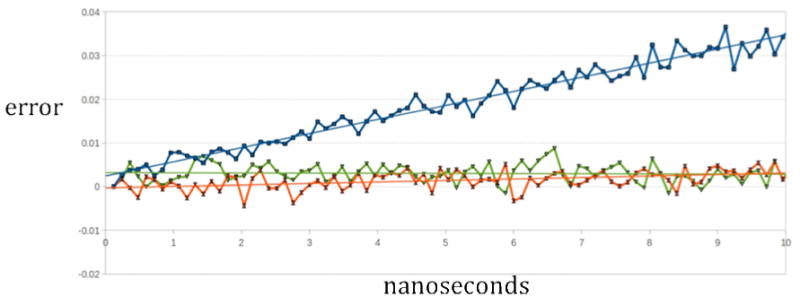
Energy drift for DHFR expressed as percentage of the relative error. We plot [100 ((E_t-E₀)/E₀)] (where E_t is the energy at time t and E₀ is the initial energy) as a function of time given in nanoseconds. Data are obtained from 10 nanosecond simulations. Blue squares correspond to 6^th entry in table 2 (PME 64SP, Quad-4096, NB Force add SP, SHAKE all bonds). Green triangles correspond to 1^st entry in table 2 (PME 64DP, Quad-4096, NB Force add DP, SHAKE all bonds) and orange hourglass to third entry in table 2 (PME 64DP, Quad-4096, NB Force add SP, SHAKE all bonds). The linear regression lines (same colors) can be interpolated to 1000 ns to get the drift per microsecond (values in column 6 of table 2). Since |E₀| is ∼60000, an increment on the y-axis of 0.01 is about 6 kcal/mol. Note the significant drift when Particle Meshed Ewald is computed in single precision (PME 64SP). Note also the small improvement obtained when the non-bonded interactions are added on the GPU in double precision (NB Force add DP). The linear fits of the green and orange curves have significant error in their linear slopes. The error of the linear slope of the blue curve is smaller.

If the drift is exceptionally small (as is the case in the most conserving options) the slope is hard to estimate and it is ill determined. This is because it is close to zero and even small fluctuations of the overall energy will cause significant change (with respect to zero). However, for most cases that show significant drift, the linear fit can be done accurately. We report the expected drift (using linear interpolation) in the microsecond time scale since this is the time scale we all want to be, and the fits are indeed close to linear. The drift is expressed by percentage of total change per microsecond (the total energy is about -60,000 kcal/mole). For comparison we also provide the drift reported by the authors of ACEMD in ⁸. We comment that ACEMD was reported to achieve 17.55ms/step for one core and 1 GPU while we are using 38.10ms/step. ACEMD parallelizes the reciprocal sum of the PME on the GPU. We however parallelized the PME on the CPU. Using a single core means that the PME in MOIL is run serially. We are therefore slower by a about a factor of two, but the energy conservation of our code as is shown in Table 2 is clearly better. Energy drifts reported for other leading programs ²⁵ seem at least as high as ACEMD, even though GPU was not used in the former cases.

Table 2.

A summary of different run options is given and their effect on the observed energy drift. A “*” in the Lookup column indicates that the run was done on GTS250. The symbol “**” is for runs on the GTX470. The rest of the runs were conducted on GTX480. The energy drift is expressed as percentage of the total change in a microsecond. Quad-4096 is a table lookup for non-bonded interactions with 4096 entries, Lin-8000 is a lookup table that is using linear interpolation, Quad-256 is a table with 256 entries that is using quadratic interpolation. The PME calculation is done either in double precision (DP), or in single precision (SP). The cut provides the two cutoff distances that are used in MOIL. The NB Force option is the use of single precision or double precision in adding the non-bonded interactions. SHAKE B/L are the options of SHAKING all bonds (B) or just light particles (L), which usually means hydrogen atoms. The tolerance of the SHAKE algorithm is fixed at 10^-12 relative error and the reciprocal sum of PME at 10^-9. Note that the first row in the table is the most accurate option and the observed drift is within the noise level. Note also the horrible drift seen with 1fs time step and without the application of SHAKE (all water molecules are kept rigid with a Matrix SHAKE algorithm). ACEMD results are taken from reference⁸ for 1fs time step. Note that we tried two grid sizes for the reciprocal sum calculations, grid size of 32 and 64 points at each Cartesian direction. The effect on energy conservation was very small. Grid size impacts, however, pair correlation functions and appropriate choice must be made for the specific system at hand. See text for more details.

			NB Force	ShakeB/L	DRIFT
Lookup	PME	Cut (box-calc)	add	(tol 10-12)	(%microsec)
Quad-4096	DP64	10.37-9.5	DP	B	0.016
Quad-4096	DP64	9.8-9.0	DP	L	0.053
*Quad-4096	DP64	10.37-9.5	SP	B	0.27
Quad-4096	DP64	8.89-8.5	SP	B	0.52
Lin-8000	DP64	10.37-9.5	SP	B	0.82
*Quad-4096	SP64	10.37-9.5	SP	B	3.2
Quad-256	SP32	8.89-8.5	SP	L	2.4
Quad-256	DP32	8.89-8.5	SP	L	0.84
**Quad-256	DP32	8.89-8.5	SP	L	-0.60
**Quad-256	SP52	8.89-8.5	SP	L	3.57
**Quad-256	DP52	8.89-8.5	SP	L	-0.30
Lin-8000	SP32	N/A-8.9	SP	NO	40.
Quad-4096	SP32	8.89-8.5	SP	NO	43.0
*Quad-4096	DP64	9.8-9.0	SP	NO	32.0
ACEMD				NO	10.15

The factors that influence energy conservation are: (i) The accuracy of the lookup table, controlled by the number of entries and level of interpolation, we consider linear interpolation with 8,000 entries, and quadratic interpolation with 4,096 and 256 table entries. (ii) the single/double precision calculations of the PME, (iii) cutoff distance (iv) single or double precision of the summation of real non-bonded force on the GPU, and (v) use of SHKL versus shaking all bonds,.

The two most important factors to achieve good energy conservation in the sub-microsecond time scale are the accuracy of the PME reciprocal sum and the SHAKE calculations. Both must be conducted in double precision. At present we also use double precision arithmetic in the calculation of the covalent energies and forces and in the numerical integration of the equations of motion, since the computational cost of these terms is negligible and there is no reason not to use double precision. In fact the only term that is not conducted in double precision in our code is the calculation of real space non-bonded interactions (on the GPU). Executing the final sum of these interactions in double precision helps and brings energy conservation to the microsecond domain, but at some computational cost.

We comment that in Milestoning calculations of long time kinetics the trajectories used are relatively short. For example, in the calculation of the recovery stroke in myosin (a millisecond process) only sub-nanosecond trajectories were used⁴. Hence, energy conservation in the nanosecond time scale may be sufficient for the theory-based long time dynamics and kinetic calculations of MOIL.

IV. Concluding remarks

We describe an implementation of MOIL-opt a version of the dynamics module of the program MOIL¹¹ that was ported to a high performance laboratory tool, namely a CPU with several cores (we used up to four) and a GPU card. The new features of the present implementation include a novel implementation of a lookup table, careful partitioning of the work between the GPU and a shared memory multi-core system, and detailed analysis of the energy conservation of the simulation. It is shown that the prime factor for successful energy conservation is the calculations of the reciprocal space of the Ewald summation in double precision. The double precision summation of the non-bonded interactions on the GPU comes next.

MOIL strongly emphasizes the calculations of reaction mechanisms and kinetics. It provides a set of tools to compute reaction paths, approximate long time trajectories, and more recently also the tools of Milestoning. Using a midrange graphic card, a system can be built that provides both high-end performance and accurate energies. Sampling correctly from the microcanonical ensemble and the production of energy conserving trajectories is necessary for estimating microscopic time scales and rates. Others used stochastic dynamics to overcome the energy drift. However, it is not clear if a stochastic dynamics, which employs a basic integrator that does not conserve energy even at the zero friction limit, produces configurations with probability p(x) proportional to exp(−U(x)/kT) This is in contrast to a Monte Carlo algorithm in which by rejections and acceptances of steps the Boltzmann distribution is enforced.

We emphasize that we do no object (of course) for stochastic dynamics to obtain sampling from ensembles other than microcanonical if the differential equations are solved exactly. However, information about microscopic kinetics is better obtained from microcanonical calculations. Even if the canonical ensemble is obtained, the addition of stochastic forces can significantly affect the time scale of the processes we study. For example, in the strong friction limit the rate constant is inversely proportional to the friction coefficient of the Langevin equation. The friction coefficient is typically determined as a phenomenological (not microscopic) parameter.

The program MOIL including the recent addition to it: MOIL-opt, is freely available from http://clsb.ices.utexas.edu/prebuilt/.

Figure 1.

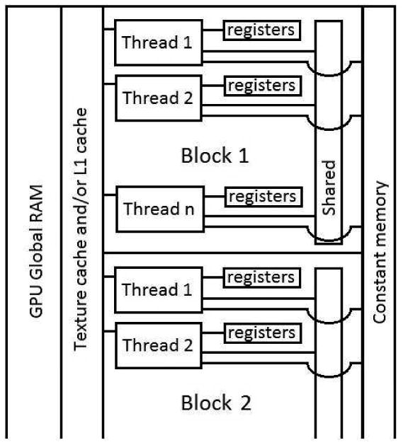
Conceptual memory layout of a CUDA GPU. Note the memory hierarchy in which the registers and shared memory are closest to the thread in the figure indicating fastest access. Registers are visible only to individual threads while shared memory is accessible to a whole block of threads. Constant memory, texture cache and L1 cache are accessible to all threads. Texture and L1 memory serve as cache on global RAM. Data completely residing in texture cache, L1 cache or constant memory also benefits from fast access. Note that each of these memories is small and texture and constant memory are read only. Direct access to global RAM is slowest although coalescing can significantly improve its performance.

Table 1.

A summary of the computational costs required to run different components of MOIL-opt for different molecular systems. Only the components with highest costs are shown. The cost is expressed in milliseconds per step with the exception of the last column (nanoseconds per day). The results in this table were obtained using 4 cores in CPU. For peptide I only 3 cores were used. “Nb real” means the real part of the nonbonded interactions which is computed on the GPU. “Nb receip” is the Ewald reciprocal sum which is calculated on the CPU. “List gene” is the generation of the neighbor list computed on the GPU. “SHAKE” is the enforcement of constraints, typically keeping water molecules rigid and fixing bond lengths between pairs of particles, one of which is hydrogen atom. The “Total” is the number of nanoseconds produced in a day of calculation. See text for more details on the simulations.

	Nb real	Nb recip	List gene	SHAKE	Total
DHFR(23,536 atoms)	7.80ms/step	7.19ms/step	1.24ms/step	2.47ms/step	4.5ns/day
Membrane (38,802 atoms	16.40	8.3	2.16	1.76	3.18
Peptide I (20,235 atoms)	12.20	8.32	1.12	1.62	3.7
Trp zipper (5,847 atoms)	2.2	1.73	0.5	0.41	45.0
Peptide II (2,690 atoms)	1.30	0.23	0.20	0.13	44.1

References

- 1.Olender R, Elber R. Calculation of classical trajectories with a very large time step: Formalism and numerical examples. J Chem Phys. 1996;105(20):9299–9315. [Google Scholar]
- 2.Dellago C, Bolhuis PG, Geissler PL. Adv Chem Phys. Vol. 123. John Wiley & Sons Inc; New York: 2002. Transition path sampling; pp. 1–78. [Google Scholar]
- 3.(a) Faradjian AK, Elber R. Computing time scales from reaction coordinates by milestoning. J Chem Phys. 2004;120(23):10880–10889. doi: 10.1063/1.1738640. [DOI] [PubMed] [Google Scholar]; (b) Majek P, Elber R. Milestoning without a Reaction Coordinate. J Chem Theory Comput. 2010;6(6):1805–1817. doi: 10.1021/ct100114j. [DOI] [PMC free article] [PubMed] [Google Scholar]; (c) Moroni D, Bolhuis PG, van Erp TS. Rate constants for diffusive processes by partial path sampling. J Chem Phys. 2004;120(9):4055–4065. doi: 10.1063/1.1644537. [DOI] [PubMed] [Google Scholar]; (d) van Erp TS, Moroni D, Bolhuis PG. A novel path sampling method for the calculation of rate constants. J Chem Phys. 2003;118(17):7762–7774. [Google Scholar]; (e) Allen RJ, Frenkel D, ten Wolde PR. Forward flux sampling–type schemes for simulating rare events: Efficiency analysis. J Chem Phys. 2006;124(19):17. doi: 10.1063/1.2198827. [DOI] [PubMed] [Google Scholar]
- 4.Elber R, West A. Atomically detailed simulation of the recovery stroke in myosin by Milestoning. Proc Natl Acad Sci USA. 2010;107:5001–5005. doi: 10.1073/pnas.0909636107. [DOI] [PMC free article] [PubMed] [Google Scholar]
- 5.Darden T, York D, Pedersen L. Particle mesh ewald – an n.log(n) method for ewald sums in large systems. J Chem Phys. 1993;98(12):10089–10092. [Google Scholar]
- 6.Tuckerman M, Berne BJ, Martyna GJ. Reversible multiple time scale molecular–dynamics. J Chem Phys. 1992;97(3):1990–2001. [Google Scholar]
- 7.(a) Shaw DE, Maragakis P, Lindorff–Larsen K, Piana S, Dror RO, Eastwood MP, Bank JA, Jumper JM, Salmon JK, Shan YB, Wriggers W. Atomic–Level Characterization of the Structural Dynamics of Proteins. Science. 2010;330(6002):341–346. doi: 10.1126/science.1187409. [DOI] [PubMed] [Google Scholar]; (b) Stone JE, Phillips JC, Freddolino PL, Hardy DJ, Trabuco LG, Schulten K. Accelerating molecular modeling applications with graphics processors. J Comput Chem. 2007;28(16):2618–2640. doi: 10.1002/jcc.20829. [DOI] [PubMed] [Google Scholar]
- 8.Harvey MJ, Giupponi G, De Fabritiis G. ACEMD: Accelerating Biomolecular Dynamics in the Microsecond Time Scale. J Chem Theory Comput. 2009;5(6):1632–1639. doi: 10.1021/ct9000685. [DOI] [PubMed] [Google Scholar]
- 9.Ravikant DVS, Elber R. PIE–efficient filters and coarse grained potentials for unbound protein–protein docking. Proteins: Struct, Funct, Bioinf. 2010;78(2):400–419. doi: 10.1002/prot.22550. [DOI] [PMC free article] [PubMed] [Google Scholar]
- 10.Anderson JA, Lorenz CD, Travesset A. General purpose molecular dynamics simulations fully implemented on graphics processing units. J Comput Phys. 2008;227(10):5342–5359. [Google Scholar]
- 11.Elber R, Roitberg A, Simmerling C, Goldstein R, Li HY, Verkhivker G, Keasar C, Zhang J, Ulitsky A. Moil a program for simulations of macrmolecules. Comput Phys Commun. 1995;91(1–3):159–189. [Google Scholar]
- 12.Elber R, Ghosh A, Cardenas A. Long time dynamics of complex systems. Acc Chem Res. 2002;35(6):396–403. doi: 10.1021/ar010021d. [DOI] [PubMed] [Google Scholar]
- 13.(a) Ryckaert JP, Ciccotti G, Berendsen HJC. Numerical integration of cartesian equations of m otion of a system with constraints – molecular dynamics of N–alkanes. J Comput Phys. 1977;23(3):327–341. [Google Scholar]; (b) Weinbach Y, Elber R. Revisiting and parallelizing SHAKE. J Comput Phys. 2005;209(1):193–206. [Google Scholar]
- 14.van Meel JA, Arnold A, Frenkel D, Zwart SFP, Belleman RG. Harvesting graphics power for MD simulations. Mol Simul. 2008;34(3):259–266. [Google Scholar]
- 15.Harvey MJ, De Fabritiis G. An Implementation of the Smooth Particle Mesh Ewald Method on GPU Hardware. J Chem Theory Comput. 2009;5(9):2371–2377. doi: 10.1021/ct900275y. [DOI] [PubMed] [Google Scholar]
- 16.Morrone JA, Zhou RH, Berne BJ. Molecular Dynamics with Multiple Time Scales: How to Avoid Pitfalls. J Chem Theory Comput. 2010;6(6):1798–1804. doi: 10.1021/ct100054k. [DOI] [PubMed] [Google Scholar]
- 17.Schnieders MJ, Fenn TD, Pande VS. Polarizable Atomic Multipole X–Ray Refinement: Particle Mesh Ewald Electrostatics for Macromolecular Crystals. J Chem Theory Comput. 2011;7(4):1141–1156. doi: 10.1021/ct100506d. [DOI] [PubMed] [Google Scholar]
- 18.Yip V, Elber R. Calculation of a list of neighbors in molecular–dynamics simulations. J Comput Chem. 1989;10(7):921–927. [Google Scholar]
- 19.Eastman P, Pande VS. Efficient Nonbonded Interactions for Molecular Dynamics on a Graphics Processing Unit. J Comput Chem. 2010;31(6):1268–1272. doi: 10.1002/jcc.21413. [DOI] [PMC free article] [PubMed] [Google Scholar]
- 20.Kaminski G, Friesner R, Tirado–Rives J, Jorgensen WL. Evaluation and reparameterization of the OPLS–AA force field for proteins via comparison with accurate quantum chemical calculations on peptides. J Phys Chem B. 2001;105(28):6474–6487. [Google Scholar]
- 21.Jorgensen WL, Chandrasekhar J, Madura JD, Impey RW, Klein ML. Comparison of simple potential functions for simulating liquid water. J Chem Phys. 1983;79(2):926–935. [Google Scholar]
- 22.Berendsen HJC, Grigera JR, Straatsma TP. The missing term in effective pair potentials. J Phys Chem. 1987;91(24):6269–6271. [Google Scholar]
- 23.(a) Jorgensen WL, Tiradorives J. The OPLS potential functions for proteins – energy minimizations for crystals of cyclic–peptides and crambin. J Am Chem Soc. 1988;110(6):1657–1666. doi: 10.1021/ja00214a001. [DOI] [PubMed] [Google Scholar]; (b) Berger O, Edholm O, Jahnig F. Molecular dynamics simulations of a fluid bilayer of dipalmitoylphosphatidylcholine at full hydration, constant pressure, and constant temperature. Biophys J. 1997;72(5):2002–2013. doi: 10.1016/S0006-3495(97)78845-3. [DOI] [PMC free article] [PubMed] [Google Scholar]
- 24.Gallardo IF, Webb LJ. Tethering Hydrophobic Peptides to Functionalized Self–Assembled Mono layers on Gold through Two Chemical Linkers Using the Huisgen Cycloaddition. Langmuir. 2010;26(24):18959–18966. doi: 10.1021/la1036585. [DOI] [PubMed] [Google Scholar]
- 25.Hess B, Kutzner C, van der Spoel D, Lindahl E. GROMACS 4: Algorithms for highly efficient, load–balanced, and scalable molecular simulation. J Chem Theory Comput. 2008;4(3):435–447. doi: 10.1021/ct700301q. [DOI] [PubMed] [Google Scholar]
Associated Data
This section collects any data citations, data availability statements, or supplementary materials included in this article.