

Abstract
Near-Infrared Spectroscopy (NIRS) measures the functional hemodynamic response occuring at the surface of the cortex. Large pial veins are located above the surface of the cerebral cortex. Following activation, these veins exhibit oxygenation changes but their volume likely stays constant. The back-reflection geometry of the NIRS measurement renders the signal very sensitive to these superficial pial veins. As such, the measured NIRS signal contains contributions from both the cortical region as well as the pial vasculature. In this work, the cortical contribution to the NIRS signal was investigated using (1) Monte Carlo simulations over a realistic geometry constructed from anatomical and vascular MRI and (2) multimodal NIRS-BOLD recordings during motor stimulation. A good agreement was found between the simulations and the modeling analysis of in vivo measurements. Our results suggest that the cortical contribution to the deoxyhemoglobin signal change (ΔHbR) is equal to 16–22% of the cortical contribution to the total hemoglobin signal change (ΔHbT). Similarly, the cortical contribution of the oxyhemoglobin signal change (ΔHbO) is equal to 73–79% of the cortical contribution to the ΔHbT signal. These results suggest that ΔHbT is far less sensitive to pial vein contamination and therefore, it is likely that the ΔHbT signal provides better spatial specificity and should be used instead of ΔHbO or ΔHbR to map cerebral activity with NIRS. While different stimuli will result in different pial vein contributions, our finger tapping results do reveal the importance of considering the pial contribution.
Keywords: NIRS-fMRI, Pial vasculature, Balloon Model, Monte Carlo simulations
1. Introduction
Near-infrared spectroscopy (NIRS) (Villringer et al., 1993; Hoshi, 2007; Hillman, 2007) is a non-invasive technique for monitoring the hemodynamic changes occuring in superficial regions of the cortex. Using non-ionizing light, NIRS measures the fluctuations of the two dominant biological chromophores in the near-infrared spectrum: oxygenated (HbO) and deoxygenated or reduced hemoglobin (HbR).
Over the past 15 years, NIRS has become an attractive alternative to functional Magnetic Resonance Imaging (fMRI), with several clinical advantages (Irani et al., 2010). NIRS is portable and less susceptible to movement artifacts enabling long term monitoring of the hemodynamic activity at the bedside. However, the spatial resolution of NIRS is 1–3 cm (Boas et al., 2004) which is less than the resolution of standard fMRI scanners. Another disadvantage of NIRS is its penetration depth which limits its sensitivity to the upper 1 cm of the cerebral cortex (Boas et al., 2004).
The biophysical origin of the functional NIRS signal is the variation of HbO and HbR concentration resulting from changes in Cerebral Blood Flow (CBF) and Cerebral Metabolic Rate of Oxygen (CMRO2). For evoked brain activity, the resulting variations in HbO and HbR are described by the Balloon model (Buxton et al., 1998; Friston, 2000; Buxton et al., 2004). According to this model, the arterial dilation driven increase in CBF following brain activation induces a passive volume increase of the capillary and venous vasculature (termed the windkessel compartment) as well as an increase in oxygen saturation. Compartmental microscopic hemodynamic measurements (Hillman et al., 2007; Drew et al., 2011) have revealed that this evoked oxygenation increase propagates through the pial veins located at the surface of the cortex but that this pial compartment exhibits very little volume variation following brain activation. This pial vein signal is generally negligible in fMRI since the high anatomical resolution allows the signal coming from the cortical region to be isolated. Conversely, the NIRS signal is integrated through the different superficial layers of the head. This potentially gives rise to a pial vein contamination of the signal if the pial vessels happen to coincide with the path of the light during its propagation through the tissue.
Preliminary analysis of the impact of pial vasculature in NIRS has been performed by Dehaes et al. (2011). However, very few studies of the effect of pial vein oxygenation changes (termed “the washout effect”) on the NIRS signal have been performed (Firbank et al., 1998; Huppert et al., 2009).
In this paper, the effect of pial vein contamination of the NIRS signal is investigated over the motor cortex where superficial pial veins are present (Gray, 2000). We first quantify cortical and pial vein contributions to the NIRS signal by Monte Carlo simulation performed on a realistic anatomical volume containing pial veins acquired with MRI. We then use a biophysical model of the fMRI signal to analyze concurrent NIRS-fMRI data acquired over the motor cortex of human subjects during a finger tapping task. The cortical contribution to the HbR and HbO signals relative to the cortical contribution of the HbT signal are both estimated by fitting the biophysical model to the multimodal data.
2. Theory
We used biophysical modelling to investigate the contribution of cortical changes in HbO and HbR to the NIRS signal taken from in vivo NIRS-BOLD measurements. The Obata model (Obata et al., 2004), a refined version of the original Balloon model (Buxton et al., 1998), describes the fluctuations in the BOLD signal as a function of the changes in deoxyhemoglobin (HbR) concentration and cerebral blood volume (CBV) in a given voxel:
| (1) |
All the parameters involved in the Obata model are summarized in Table 1.
Table 1.
Parameters of the Obata model
| Symbol | Value | Description |
|---|---|---|
| V0 | - | Resting venous blood volume fraction |
| r0 | 100 s−1 | Taylor expansion of intravascular relaxation rate Δ R21 |
| ν 0 | 80.6 s−1 | Frequency offset at the surface of magnetized vessel |
| TE | 20 or 30 ms | Echo-time of the MRI sequence |
| ε | 0.59 for TE=30ms 0.70 for TE=20ms |
Intrinsic/Extrinsic signal ratio |
| E0 | 0.4 | Baseline oxygen extraction fraction |
| k 1 | 4.3 · ν0· E0· TE | Lumped constant |
| k 2 | ε·r0·E0· TE | Lumped constant |
| k 3 | ε – 1 | Lumped constant |
The general idea behind our method is the following: NIRS can measure independently variations in cerebral blood volume and in the concentration of deoxyhemoglobin. Based on the Obata model, these are the two physiological phenomena giving rise to the BOLD signal. Therefore, one could potentially predict the BOLD signal from the NIRS measurements. This idea has been investigated previously by Huppert et al. (2006b, 2009). However, the NIRS signal is contaminated by pial vein washout (Culver et al., 2005; Dehaes et al., 2011). While the pial compartment cannot be extracted from the NIRS measurements, this component can be removed from the fMRI data because of the high spatial resolution of BOLD-fMRI. Because NIRS suffers from pial contamination, the NIRS-predicted BOLD signal will agree with the measured BOLD signal only if the NIRS data are corrected for pial vein washout.
To apply the above methodology, the Obata model must be modified to account for two discrepancies between BOLD-fMRI and NIRS. (1) Continuous-wave NIRS cannot measure relative changes in hemoglobin but rather a quantity proportional to absolute variations. (2) NIRS measures variations in total hemoglobin (HbT) rather than CBV. The Obata model as written in Eq. (1) contains only dimensionless variables i.e. all the variables are normalized by their value at rest. Making use of the relation
| (2) |
where Hct represents the hematocrit and MWHb the molecular weight of hemoglobin, the Obata model can be re-written in terms of absolute hemoglobin variations which can be measured by NIRS. The new model will be referred to the NIRS-adapted Obata model:
| (3) |
with
| (4) |
and
| (5) |
The definition and value of the parameters involved in this new version are summarized in Table 2.
Table 2.
Parameters of the NIRS-adapted Obata model
| Symbol | Value | Description |
|---|---|---|
| MW Hb | 64 500 g/mol | Molecular weight of hemoglobin |
| Hct | 160 g/L | Hematocrit |
| * γ HbT | ~ 1 | Cortical weighting factor for HbT |
| * γ HbR | to be estimated | Cortical weighting factor for HbR |
| **PVCHbT | 50 | Partial volume correction factor for HbT |
| **PVCHbR | 50 | Partial volume correction factor for HbR |
| SaO2 | 0.98 | Oxygen saturation in arteries |
γ handles cortical vs pial (which are both part of the activated brain tissue)
PVC handles activated brain tissue vs scalp+skull+non-activated brain tissue
Generally, the pathlength of the light in the head can be separated into scalp and skull layers, non-activated brain tissue and activated brain tissue (Strangman et al., 2003). In this paper, we further separate the activated brain tissue into two regions: the cortical tissue and the pial vasculature. More specifically, the quantity PVC represents a partial volume correction extracting the signal coming from the activated brain tissue from the signal coming from the rest of the head (i.e. skin/skull and non-activated brain tissue crossed by the light). Finally, the variable γ represents the fraction of the activated brain tissue signal that is coming from cortical tissue while 1 − γ represents the fraction originating from pial vein oxygenation changes.
The coeffcients a1 and a2 in Eq. (3) were estimated from the multimodal data set using a standard least-square method. ΔBOLD/BOLD was extracted from the fMRI data while ΔHbT and ΔHbR were computed from the NIRS data. Once a1 and a2 were recovered, the cortical contribution of HbR relative to HbT defined as γHbRr = γHbR/γHbT was computed using the following relation:
| (6) |
where a1 and a2 were obtained from the least-square fit and the value for the rest of the parameters taken from the literature.
In our model, we separately account for the volume fraction of the activated brain tissue (with PVC) and the cortical vs pial composition of the activated tissue (with γ). With the above definition, PVC depends on the wavelengths of the NIRS sources and γ does not. Strangman et al. (2003) showed that measurements performed at 690 nm and 830 nm minimize the cross-talk between HbT and HbR introduced by incorrect values of PVC. Since these wavelengths were used in our measurements, crosstalk between HbR and HbT was negligible and it was reasonable to assume PVCHbT=PVCHbR. As such, these two factors cancel out in the estimation of with Eq. (6), as do Hct and MWHb. Our estimation of was therefore independent of the values assumed for these parameters. Under these assumptions, Eq. (6) reduces to
| (7) |
Culver et al. (2005) showed that the spatial extend of the activation region measured by HbT is smaller than the one measured by HbO or HbR. The larger activation region measured by HbO and HbR was attributed to potential washout of the deoxyhemoglobin in the pial vasculature during the activation. The same phenomenon of extended pial vein washout is handled by the parameter γ in our model. Pial veins exhibit only very small volume changes following brain activation (Culver et al., 2005; Hillman et al., 2007; Drew et al., 2011). Therefore, the value of γHbT is very close to 1 indicating that most of the HbT signal is coming from the cortical region. Under this assumption, a pure washout of HbR is observed and thus the amplitude of the pial increase in HbO matches the amplitude of the pial decrease in HbR:
| (8) |
where (1 − γ) indicates the pial fraction of the signal. One can derive the expression for the cortical weighting factor for HbO (γHbO) from Eq. (8):
| (9) |
The parameter γHbR alone cannot be extracted from the in vivo data but under the assumption that γHbT ≈ 1, the approximation holds. We will refer to as the estimation of γHbO under this assumption by substituting γHbR by in Eq. (9):
| (10) |
where the subscript “r” emphasizes the assumption of no pial volume changes.
Conversely, in the cortical tissues the amplitude of the increase in HbO does not match the decrease in HbR because vascular dilation gives rise to a change in blood volume (Buxton et al., 1998). Therefore, the cortical fraction of the signal, γ, given by the ratio of the cortical signal over the total activated tissue signal , will be di erent for HbR and HbO. Since the amplitude of the cortical ΔHbR is lower than the amplitude of the cortical ΔHbO, the relative cortical weighting factor will be lower for HbR compared to HbO ().
3. Methodology
3.1. Monte Carlo simulations
The effect of pial vein washout was first investigated using Monte Carlo simulation. The anatomical model used in the simulation was the same as in Dehaes et al. (2011). A high resolution anatomical T1 MRI image was acquired and tissues where then segmented in four different types: scalp, skull, cerebrospinal fluid (CSF) and brain tissue (containing both white and gray matter). The segementation was performed using the Matlab package SPM8. A phase contrast MR angiography was also used to image the pial vasculature located at the surface of the cortex (Dehaes et al., 2011; Moran, 1982). A saturation band was applied to suppress the arterial blood signal such that only pial veins were kept in the final anatomical model. The selected velocity encoding was 5 mm/s for the plane described by the right-left and anterior-posterior encoding. The bandwidth was 300 Hz/px and imaging times were TR/TE = 80.9/10.3 ms. The flip angle was set to 15°. More information about the sequence parameters can be found in Dehaes et al. (2011). An illustration of the anatomical model with the position of the optical sources and detectors is shown in Fig. 1.
Figure 1.

Anatomical model used in the Monte Carlo simulations. The position of the optical sources and detectors is also illustrated as well as the simulated region of activation.
Specific optical properties were assigned to each tissue type and are summarized in Table 3. These values were computed using the model from Strangman et al. (2003) which takes into account the blood content and the oxygen saturation of each tissue type. A baseline oxygen saturation of 60 % was assumed in the pial veins (Buxton, 2002). In the specific cortical region shown in red in Fig. 1, we simulated an increase in HbO of +9 μM and a decrease in HbR of −3 μM. In our simulation, we also induced an increase in oxygen saturation in the pial veins (SpO2) ranging from 5 to 10 %, as reported in the literature (Buxton, 2002; Yaseen et al., 2011).
Table 3.
Optical properties assigned to the different tissue types for the Monte Carlo simulations. Absorption coefficient μa [mm−1], scattering coefficients μs [mm−1], anisotropic factors g and refractive indexes n. The brain tissue includes gray and white matter. Values were computed using the method given in Strangman et al. (2003).
| Tissue | λ = 690 nm |
λ = 830 nm |
||||||
|---|---|---|---|---|---|---|---|---|
| μ a | μ s | g | n | μ a0 | μ s | g | n | |
| Scalp | 0.0159 | 8.000 | 0.900 | 1.4 | 0.0191 | 6.600 | 0.900 | 1.4 |
| Skull | 0.0101 | 10.00 | 0.900 | 1.4 | 0.0136 | 8.600 | 0.900 | 1.4 |
| CSF | 0.0004 | 0.100 | 0.900 | 1.4 | 0.0026 | 0.100 | 0.900 | 1.4 |
| Brain | 0.0178 | 12.50 | 0.900 | 1.4 | 0.0186 | 11.10 | 0.900 | 1.4 |
| Pial veins | 0.5745 | 74.50 | 0.985 | 1.4 | 0.4758 | 67.50 | 0.992 | 1.4 |
Monte Carlo methods were used to simulate the photon fluence at each NIRS detector (Boas et al., 2002). Fluences were computed for a baseline state i.e. using the optical properties given in Table 3 as well as for an activated state i.e. modifying slightly the optical properties of the brain tissue and the pial veins in Table 3 to take into account the cortical activation as well as the change in oxygen saturation in the pial veins. We then used the modified Beer-Lambert law (Deply et al., 1988; Cope and Deply, 1998) to recover the hemoglobin concentration changes from the fluences detected during the baseline and the activated state. In our simulations, the relationship between the HbR change simulated in the cortical region () and the total HbR change recovered at the detector () containing both cortical and pial contributions is given by
| (11) |
with the Partial Volume Correction factor (PVCHbR) relating the total detected HbR change () to the total simulated HbR change () in the brain tissue. Similar equations hold for HbT
| (12) |
and for HbO
| (13) |
Without simulating volume changes in the pial veins, γHbT = 1 and from Eq. (12) we find that . We first verified that using tissue optical properties for 690 nm and 830 nm, the partial volume correction factor (PVC) as defined in this paper was the same for HbR, HbT and HbO by running a simulation with an activation in the cortical region only i.e. γHbR = 1 and γHbO = 1 (see Fig. 2A). Once this assumption was justified, a second simulation was run with a washout effect in the pial vasculature on top of a cortical activation (see Fig. 2B). From this second simulation, the cortical weighting factor for HbR and HbO were computed using Eq. (11) with PVCHbR = PVCHbT and Eq. (13) with PVCHbO = PVCHbT respectively
| (14) |
| (15) |
Figure 2.
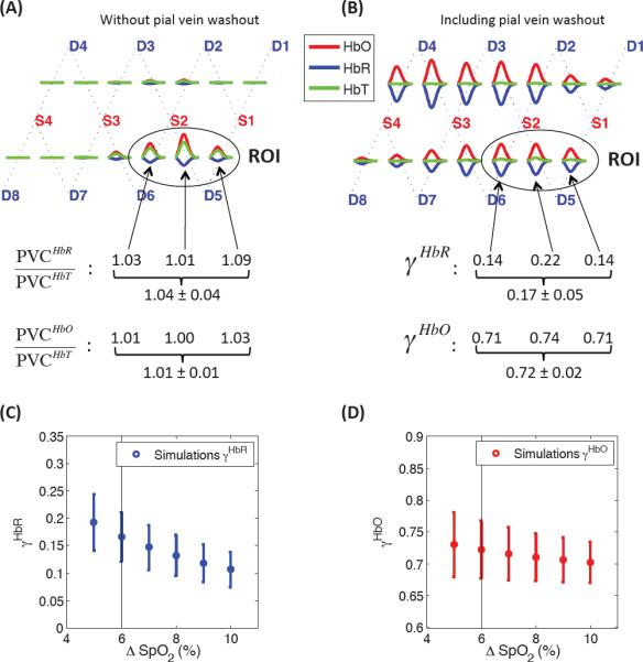
Results of the Monte Carlo simulations performed on the numerical volume shown in Fig. 1. (A) Simulation of a cortical activation with no pial vein washout (γHbR = 1 and γHbO = 1) to define the ROI and verify that PVCHbR = PVCHbT and PVCHbO = PVCHbT. (B) Simulation of a pial veins oxygenation increase of 6 % (60 to 66%) on top of a cortical activation. No volume changes were simulated in the pial veins (γHbT = 1). (C–D) Sensitivity analysis showing (C) the γHbR and (D) the γHbO values recovered by simulating an oxygenation increase of 5 to 10 %.
3.2. In vivo studies
Two different studies were performed. In each of them, we recorded concurrent NIRS-fMRI during a motor task which consisted of finger tapping blocks with a duration of either 2 s or 20 s.
In the first study, simultaneous NIRS-fMRI data were acquired during 2 s finger tapping blocks. These data have previously been described by Huppert et al. (2006a,b, 2009). Six subjects were scanned and completed six runs containing 30 individual events each. The NIRS data were bandpass filtered at 0.03–0.8 Hz before being block-averaged across all runs and all individual events. The source–detector pairs to be included in the region-of-interest average were chosen for each subject consistently with the fMRI data and from measurements showing statistically significant changes (p < 0.05). The grand average across the six subjects was then computed. The BOLD data were acquired using parameters TR/TE/θ=500 ms/30 ms/90°. The functional images were first motion corrected and spatially smoothed with a 6-mm Gaussian kernel. For each subject, a t-statistic map was generated and threshold was applied for p < 0.05. Significant voxels were then manually selected under the NIRS probe based on fiducial markers and the grand average was computed across all six subjects. The hemodynamic response functions were then calculated by an ordinary least-squares linear deconvolution with a third order polynomial drift. Each of the ΔHbO, ΔHbR, ΔHbT and ΔBOLD time courses were adjusted to cross y=0 at t=0 by subtracting their respective value at t=0.
In the second study, concurrent NIRS-ASL data were acquired during 20 s finger tapping blocks. These data have been previously published by Hoge et al. (2005). The NIRS data were bandpass filtered at 0.0167–0.5 Hz. The source–detector pairs to be included in the region-of-interest average were chosen for each subject consistently with the fMRI data and from measurements showing better than p < 0.05 significance. The grand average across the five subjects was then computed. The BOLD signal was extracted from the control images of the ASL acquisition (Hoge et al., 2005) with parameters TR/TE=2 s/20 ms. For each subject, we generated a t-statistic map to identify regions of significant response. Each t-map was thresholded at p < 0.05 to compute the hemodynamic response. This resulted in a focal ROI positioned on the precentral gyrus and located beneath the source-detector array of the optical probe. The hemodynamic responses were computed from the ROI using a linear deconvolution model with a third order polynomial drift. Each of the ΔHbO, ΔHbR, ΔHbT and ΔBOLD time courses were adjusted to cross y=0 at t=0 by subtracting their respective value at t=0.
For each study, we fitted Eq. (3) to the averaged ΔBOLD, ΔHbT and ΔHbR reponses with a least-square method to recover a1 and a2 before computing using Eq. (7). The parameter was then estimated using Eq. (10).
4. Results
4.1. Simulation results
Results of the Monte Carlo simulations are summarized in Fig. 2. Panel (A) shows the simulated concentration changes when no increase in oxygen saturation was simulated in the pial veins. Using Eqs. (11–13) with γHbR = γHbT = γHbO = 1, the PVCHbR/PVCHbT and PVCHbO/PVCHbT ratios computed were very close to 1 confirming that the Partial Volume Correction factor (PVC) was the same for HbR, HbO and HbT. The region of interest (ROI) was defined by the three source-detector pairs showing the strongest activation. Panel (B) shows the simulated concentration changes when we added a 6% increase (60 to 66 %) in oxygen saturation in the pial veins on top of the cortical activation (+9 μM ΔHbO and −3 μM ΔHbR). The average cortical weighting factor γ computed with Eqs. (14–15) and taken over the three source-detector pairs of the ROI was 0.17 (or 17 %) for HbR and 72 % for HbO. We also ran the simulation inducing different oxygenation increases in the pial veins ranging from 5 to 10 %. The γHbR values recovered in each case are shown in Fig. 2C and ranged from 11 to 19%, while the γHbO values were less sensitive and decreased from 73 % to 70 % as shown in Fig. 2D.
4.2. Modeling analysis of in vivo measurements
The average experimental time course for ΔHbO, ΔHbR, ΔHbT and ΔBOLD during functional activation are shown in Fig. 3. The and values recovered with Eqs. (7) and (10) for each data set are also shown. The value was 18% for the 2 s finger tapping study and 23% for the 20 s finger tapping study. The value was 77% for both studies. The uncertainty for was larger than because its calculation using Eq. (10) requires additional experimental measurements, which introduced additional errors.
Figure 3.

Finger tapping results. The average traces for ΔHbO, ΔHbR, ΔHbT and ΔBOLD are shown as well as the and values recovered with the NIRS-adapted Obata model. Error bars represent the standard error computed across the five subjects. (A) Study I: 2 s finger tapping. (B) Study II: 20 s finger tapping.
The value recovered in each case depends of the value assumed for six parameters: , E0, ∊, ν, r0 and SaO2. A sensitivity analysis was performed for each of these parameters and the results are shown in Fig. 4 for . Sensitivity for is not shown since was computed directly from using Eq. (10). In each case, the value of a single parameter was varied while all the other parameters were kept constant. For each parameter, the black vertical line indicates the value assigned to this parameter while varying the value of another parameter. For all parameters except ∊ (the Intrinsic/Extrinsic fMRI signal ratio), the recovered ranged between 15 and 30% when varying the Obata model parameters over a reasonable range. However, the recovery was more sensitive to the value assumed for ∊ and ranged from 10 to 100% when ∊ varied from 0.5 to 1.4.
Figure 4.

Sensitivity analysis for different parameters of the model. (A)–(F) Sensitivity of the recovered from our in vivo data for different values assumed for the Obata model parameters. Results are illustrated for both the 2 s (blue) and the 20 s (red) finger tapping studies. The vertical lines show the reference values indicated in Tables 1 and 2.
4.3. Combined results
The combined results from the simulations and the modeling of the in vivo measurements are summarized in Fig. 5. The average cortical weighting factor value was 19% ± 3% for HbR and 76% ± 3% for HbO.
Figure 5.

Summary of cortical weighting factors ( and ). Results are shown for the two in vivo studies, for the Monte Carlo simulations as well as the grand average.
5. Discussion
5.1. Cortical contribution to the NIRS signal
As shown in Fig. 5, our simulations agreed very well with our modeling results from the in vivo measurements, confirming the assumptions made in our computations. The good agreement between the γHbR values computed from simulations (where γHbT was forced to be 1) and the values computed from the experimental data indicates that γHbT modeled from the in vivo measurements was very close to 1. This result is strongly supported by exposed cortex animal imaging models (Hillman et al., 2007; Drew et al., 2011). Therefore, our in vivo results can be interpreted on the same footing as our simulations results.
Our combined results (averaged from simulations and in vivo modeling) indicate that for a task-evoked response over the motor cortex, the cortical contribution of the detected ΔHbR signal corresponds to 19% of the cortical contribution of the ΔHbT signal e.g. that the cortical contribution is 5 times smaller for ΔHbR compared to ΔHbT. For ΔHbO, this value was found to be 76%. Our results suggest that both the ΔHbO and ΔHbR signals contain a significantly higher pial vein contribution compared to ΔHbT. It is therefore likely that the ΔHbT signal will provide better spatial specificity (Sheth et al., 2004; Culver et al., 2005) and should be used instead of ΔHbO or ΔHbR to map cerebral activity with NIRS.
Since our results suggest that no pial volume change occurred, and thus our numbers indicate that 19% of the entire ΔHbR signal and 76% of the entire ΔHbO signal is coming from the cortical region. The remaining 81% and 24% of the signal for ΔHbR and ΔHbO respectively originate from the pial veins located at the surface of the motor cortex, where a change in oxygen saturation takes place following brain activation. This finding is not surprising since NIRS exhibits a sensitivity profile that exponentially decreases with depth (Boas et al., 2004) and the pial vasculature is located above the surface of the cortex.
Previous work by Huppert et al. (2009) using the same data set used in our first study (2 s tapping) found that 44% of the NIRS signal (accouting for both HbO and HbR) was coming from the cortical region. Taking the average of our and value gives 48% which agrees well with this value.
Our sensitivity analysis revealed that the values found from the in vivo data were not very sensitive to the parameters assumed in the Obata model, except for the ∊ parameter representing the Intrinsic/Extrinsic fMRI signal ratio. Assuming larger ∊ values would change our results by increasing as shown in Fig. 4C. However, recent work by Griffeth and Buxton (2011) supports the accuracy of our results by reporting similar ∊ values to those used in our study. Using a detailed analysis, Griffeth and Buxton showed that for TE=32 ms, the ∊ value is close to 0.5 in veins and goes up to 1 and 1.3 in the capillaries and the arteries respectively. In our work, the arterial compartment was assumed negligible since most of the BOLD signal is coming from the veins. The capillary compartment was combined with the veins in a single compartment model as in Obata et al. (2004). Using the equations in Obata et al, we computed an effective ∊ value of 0.58 and 0.7 for TE=30 ms and TE=20 ms respectively, which agrees well with Griffeth and Buxton's findings.
5.2. Impact on NIRS-fMRI CMRO2 estimation
Our results suggest that caution must be taken in quantifying cortical cerebral activity from NIRS measurements acquired over a region where large pial veins are located. If concurrent fMRI data are available, the NIRS-adapted Obata model (Eq. 3) allows us to compute the cortical contribution under some realistic assumptions.
The Cerebral Metabolic Rate of Oxygen (CMRO2) can be estimated from concurrent NIRS-fMRI recordings (Hoge et al., 2005; Huppert et al., 2009). The pial compartment was already taken into account in Huppert et al. (2009)'s computation. In Hoge et al (Hoge et al., 2005), CMRO2 was computed from the NIRS data without any corrections for pial vein washout. CMRO2 was given by the product of the change in oxygen extraction fraction (E) and the change in CBF: rCMRO2 = rE × rCBF, where r denotes a quantity normalized by its baseline value. The change in CBF was estimated from the ASL data while the change in oxygen extraction fraction was computed from the NIRS data: rE = rHbR/rHbT. Following activation, CBF increases (rCBF > 1) and the oxygen extraction fraction decreases (rE < 1) (Buxton et al., 1998). Correcting rHbR for the pial contamination lowers the decrease in HbR resulting in a higher rE and a higher rCMRO2. Depending on the baseline hemoglobin concentrations, this correction can be significant. With the values given in Hoge et al. (2005), the pial vein correction increases rCMRO2 by 15% (from 1.40 to 1.61) while this value increased from 1.26 to 1.49 assuming a lower baseline oxygen saturation measured by time-resolved spectroscopy (Gagnon et al., 2008).
5.3. Limitations and future studies
The values for the oxygenation increase induced in the pial veins in our Monte Carlo simulation were taken from the literature (Buxton, 2002; Yaseen et al., 2011). This was necessary since we did not monitor the response in the pial veins during our fMRI scans. Future studies could use magnetic resonance susceptometry-based oximetry (Jain et al., 2010) to monitor oxygen saturation in the pial veins following activation. These values would be more accurate than the ones computed from a simplified model and could be used in the Monte Carlo simulations to give more accurate results.
In our analysis, we have ignored any global systemic flow variations in the skin that could be phase-locked with the hemodynamic response in the brain. These flow changes in the skin potentially contaminate the NIRS signal because of its high sensitivity to superficial tissues. If true, these contributions would have simply been integrated with the pial vein washout (1 − γ) in our in vivo analysis without changing the conclusion of this paper. However, we have completely ignored any skin contributions in our MC simulations. Such skin artefact should also be considered in future work. Preliminary work by Kirilina et al. (2011) analysed the fMRI response in the skin located under a NIRS probe and was able to relate these responses to artefacts in the NIRS signal acquired on the forehead.
Our setup did not allow us to acquire a pial angiogram and functional data on the same subjects. Even though our simulation results matched our in vivo analysis, we could not assess inter-subject vascular-based variability. Future multimodal studies will be required to quantify how the geometry of the vasculature impacts the NIRS signal. Preliminary work by Perdue and Diamond (2011) has shown that the inter-subject variability of NIRS can be partially attributed to anatomical vasculature differences.
Our study was performed over the motor cortex where pial vasculature is known to be present at the surface. Other regions might exhibit stronger contamination due to larger vessels, such as the sagittal sinus in the visual cortex (Dehaes et al., 2011), or weaker contamination due to smaller vessels as in the forehead. Future studies will be required to map the contribution of the pial vasculature in the NIRS signal across different regions of the brain.
6. Conclusion
We have shown that the NIRS signal collected over the motor cortex during an evoked task contained a smaller cortical contribution for ΔHbR and ΔHbO compared to ΔHbT. The cortical contribution to ΔHbR was equal to 19% of the cortical contribution to ΔHbT. Similarly, the cortical contribution to ΔHbO was equal to 76% of the cortical contribtion to ΔHbT. Our results suggest that the pial contamination is less important for ΔHbT, and therefore, the ΔHbT signal should be used rather than ΔHbO or ΔHbR to map cerebral activity with NIRS. This pial vein contamination has a significant impact on the quantification of cerebral activity using NIRS and correction factors must be applied in order to compute CMRO2 from concurrent NIRS-fMRI measurements.
Research Highlights.
Pial vasculature contaminates the NIRS signal
Concurrent NIRS-fMRI recordings allows to estimate cortical signal contribution 20 % of HbR signal and 75 % of HbO signal has cortical origins (finger tapping) HbT should be used rather than HbO or HbR to map cerebral activity with NIRS
Acknowledgements
We want to thank Qianqian Fang for providing the Monte Carlo code used in this study as well as providing useful advice. The authors are also grateful to Sungho Tak, Yunjie Tong, Blaise deB. Frederick and Evgeniya Kirilina for fruitful discussions. This work was supported by NIH grants P41-RR14075 and R01-EB006385. L. Gagnon was supported by the Fonds Quebecois sur la Nature et les Technologies.
Footnotes
Publisher's Disclaimer: This is a PDF file of an unedited manuscript that has been accepted for publication. As a service to our customers we are providing this early version of the manuscript. The manuscript will undergo copyediting, typesetting, and review of the resulting proof before it is published in its final citable form. Please note that during the production process errors may be discovered which could affect the content, and all legal disclaimers that apply to the journal pertain.
References
- Boas D, Culver J, Stott J, Dunn A. Three dimensional monte carlo code for photon migration through complex heterogenous media including the adult human head. Opt. Express. 2002;10(3):159–170. doi: 10.1364/oe.10.000159. [DOI] [PubMed] [Google Scholar]
- Boas D, Dale AM, Franceschini MA. Diffuse optical imaging of brain activation: Approaches to optimizing image sensitivity, resolution and accuracy. NeuroImage. 2004;23:S275–S288. doi: 10.1016/j.neuroimage.2004.07.011. [DOI] [PubMed] [Google Scholar]
- Buxton R, Wong E, Frank L. Dynamics of blood flow and oxygenation changes during brain activation: the balloon model. Magn. Reson. Med. 1998;39(6):855–864. doi: 10.1002/mrm.1910390602. [DOI] [PubMed] [Google Scholar]
- Buxton RB. Introduction to Functional Magnetic Resonance Imaging: Principles and Techniques. Cambridge University Press; 2002. [Google Scholar]
- Buxton RB, Uludag K, Dubowitz DJ, Liu TT. Modeling the hemodynamic response to brain activation. NeuroImage. 2004;23:S220–S233. doi: 10.1016/j.neuroimage.2004.07.013. [DOI] [PubMed] [Google Scholar]
- Cope M, Deply DT. System for long-term measurement of cerebral blood flow and tissue oxygenation on newborn infants by infrared transillumination. Med. Biol. Eng. Comput. 1998;26:289–294. doi: 10.1007/BF02447083. [DOI] [PubMed] [Google Scholar]
- Culver JP, Siegel AM, Franceschini MA, Mandeville JB, Boas DA. Evidence that cerebral blood volume can provide brain activation maps with better spatial resolution than deoxygenated hemoglobin. NeuroImage. 2005;27(4):947–59. doi: 10.1016/j.neuroimage.2005.05.052. [DOI] [PubMed] [Google Scholar]
- Dehaes M, Gagnon L, Lesage F, Pelegrini-Issac M, Vignaud A, Valabregue R, Grebe R, Wallois F, Benali H. Quantitative investigation of the effect of the extra-cerebral vasculature in diffuse optical imaging: a simulation study. Biomedical Optics Express. 2011;2(3):680–695. doi: 10.1364/BOE.2.000680. [DOI] [PMC free article] [PubMed] [Google Scholar]
- Deply DT, Cope M, van der Zee P, Arridge S, Wray S, Wyatt J. Estimation of optical pathlength through tissue from direct time of flight measurement. Phys. Med. Biol. 1988;33:1433–1442. doi: 10.1088/0031-9155/33/12/008. [DOI] [PubMed] [Google Scholar]
- Drew PJ, Shih AY, Kleinfeld D. Fluctuating and sensory-induced vasodynamics in rodent cortex extend arteriole capacity. Proc Natl Acad Sci USA. 2011;108(20):8473–8478. doi: 10.1073/pnas.1100428108. [DOI] [PMC free article] [PubMed] [Google Scholar]
- Firbank M, Okada E, Delpy DT. A theoretical study of the signal contribution of regions of the adult head to near-infrared spectroscopy studies of visual evoked responses. NeuroImage. 1998;8(1):69–78. doi: 10.1006/nimg.1998.0348. [DOI] [PubMed] [Google Scholar]
- Friston K. Nonlinear responses in fMRI: The balloon model, volterra kernels, and other hemodynamics. NeuroImage. 2000;12(4):466–477. doi: 10.1006/nimg.2000.0630. [DOI] [PubMed] [Google Scholar]
- Gagnon L, Gauthier C, Selb J, Boas DA, Hoge RD, Lesage F. Double layer estimation of intra- and extra-cerebral hemoglobin concentration with a time-resolved system. J. Biomed. Opt. 2008;13(5):054019. doi: 10.1117/1.2982524. [DOI] [PMC free article] [PubMed] [Google Scholar]
- Gray H. Anatomy of the Humain Body. Lea & Febiger; Philadelphia: 2000. [Google Scholar]
- Griffeth VE, Buxton RB. A theoretical framework for estimating cerebral oxygen metabolism changes using the calibrated-BOLD method: Modeling the effects of blood volume distribution, hematocrit, oxygen extraction fraction, and tissue signal properties on the BOLD signal. NeuroImage. 2011;1(1):198–212. doi: 10.1016/j.neuroimage.2011.05.077. [DOI] [PMC free article] [PubMed] [Google Scholar]
- Hillman E, Devor A, Bouchard M, Dunn A, Krauss G, Skoch J, Bacskai B, Dale A, Boas D. Depth-resolved optical imaging and microscopy of vascular compartment dynamics during somatosensory stimulation. NeuroImage. 2007;35(1):89–104. doi: 10.1016/j.neuroimage.2006.11.032. [DOI] [PMC free article] [PubMed] [Google Scholar]
- Hillman EMC. Optical brain imaging in vivo: techniques and applications from animal to man. J. Biomed. Opt. 2007;12(5):051402. doi: 10.1117/1.2789693. [DOI] [PMC free article] [PubMed] [Google Scholar]
- Hoge RD, Franceschini MA, Covolan RJM, Huppert T, Mandeville JB, Boas DA. Simultaneous recording of task-induced changes in blood oxygenation, volume, and flow using diffuse optical imaging and arterial spin-labeling mri. NeuroImage. 2005;25:701–707. doi: 10.1016/j.neuroimage.2004.12.032. [DOI] [PubMed] [Google Scholar]
- Hoshi Y. Functional near-infrared spectroscopy: current status and future prospects. J. Biomed. Opt. 2007;12(6):062106. doi: 10.1117/1.2804911. [DOI] [PubMed] [Google Scholar]
- Huppert T, Hoge R, Dale AM, Franceschini M, Boas D. Quantitative spatial comparison of diffuse optical imaging with blood oxygen level-dependent and arterial spin labeling-based functional magnetic resonance imaging. J. Biomed. Opt. 2006a;11(6):064018. doi: 10.1117/1.2400910. [DOI] [PMC free article] [PubMed] [Google Scholar]
- Huppert T, Hoge R, Diamond S, Franceschini M, Boas D. A temporal comparison of BOLD, ASL, and NIRS hemodynamic responses to motor stimuli in adult humans. NeuroImage. 2006b;29:368–382. doi: 10.1016/j.neuroimage.2005.08.065. [DOI] [PMC free article] [PubMed] [Google Scholar]
- Huppert TJ, Allen MS, Diamond SG, Boas DA. Estimating cerebral oxygen metabolism from fmri with a dynamic multicompartment windkessel model. Hum. Brain Mapp. 2009;30(5):1548–1567. doi: 10.1002/hbm.20628. [DOI] [PMC free article] [PubMed] [Google Scholar]
- Irani F, Platek SM, Bunce S, Ruocco AC, Chute D. Functional near infrared spectroscopy (fNIRS): An emerging neuroimaging technology with important applications for the study of brain disorders. The Clinical Neuropsychologist. 2010;21(1):9–37. doi: 10.1080/13854040600910018. [DOI] [PubMed] [Google Scholar]
- Jain V, Langham MC, Wehrli FW. MRI estimation of global brain oxygen consumption rate. J. Cereb. Blood Flow Metab. 2010;30(9):1598–1607. doi: 10.1038/jcbfm.2010.49. [DOI] [PMC free article] [PubMed] [Google Scholar]
- Kirilina E, Jelzow A, Heine A, Niessing M, Jacobs A, Wabritz H, Macdonald R, Bruehl R, Ittermann B, Tachtsidis I. The physiological origin of task-evoked artifacts in functional near infrared spectroscopy. 17th Annual Meeting of the Organization for Human Brain Mapping; Quebec City. 2011. [Google Scholar]
- Moran P. A flow velocity zeugmatographic interlace for nmr imaging in humans. Mag. Res. Med. 1982;1:197–203. doi: 10.1016/0730-725x(82)90170-9. [DOI] [PubMed] [Google Scholar]
- Obata T, Liu T, Miller K, Luh W, Wong E, Frank L, Buxton R. Discrepancies between BOLD and flow dynamics in primary and supplementary motor areas: application of the balloon model to the interpretation of BOLD transients. NeuroImage. 2004;21(1):144–153. doi: 10.1016/j.neuroimage.2003.08.040. [DOI] [PubMed] [Google Scholar]
- Perdue KL, Diamond SG. Anatomical vasculature modeling for functional near-infrared spectroscopy. 17th Annual Meeting of the Organization for Human Brain Mapping; Quebec City. 2011. [Google Scholar]
- Sheth S, Nemoto M, Guiou M, Walker M, Pouratian N, Hageman N, Toga A. Columnar specificity of microvascular oxygenation and volume responses: implications for functional brain mapping. J. of Neuroscience. 2004;24(3):634. doi: 10.1523/JNEUROSCI.4526-03.2004. [DOI] [PMC free article] [PubMed] [Google Scholar]
- Strangman G, Franceschini MA, Boas DA. Factors affecting the accuracy of near-infrared spectroscopy concentration calculations for focal changes in oxygenation parameters. NeuroImage. 2003;18:865–879. doi: 10.1016/s1053-8119(03)00021-1. [DOI] [PubMed] [Google Scholar]
- Villringer A, Hock C, Schleinkofer L, Dirnagl U. Near infrared spectroscopy (NIRS): A new tool to study hemodynamic changes during activation of brain function in human adults. Neurosci. Lett. 1993;154:101–104. doi: 10.1016/0304-3940(93)90181-j. [DOI] [PubMed] [Google Scholar]
- Yaseen MA, Srinivasan VJ, Sakadžić S, Radhakrishnan H, Gorczynska I, Wu W, Fujimoto JG, Boas DA. Microvascular oxygen tension and flow measurements in rodent cerebral cortex during baseline conditions and functional activation. J Cereb Blood Flow Metab. 2011;31:1051–1063. doi: 10.1038/jcbfm.2010.227. [DOI] [PMC free article] [PubMed] [Google Scholar]