Real-space processing of helical filaments in SPARX

Abstract

We present a major revision of the iterative helical real-space refinement (IHRSR) procedure and its implementation in the SPARX single particle image processing environment. We built on over a decade of experience with IHRSR helical structure determination and we took advantage of the flexible SPARX infrastructure to arrive at an implementation that offers ease of use, flexibility in designing helical structure determination strategy, and high computational efficiency. We introduced the 3D projection matching code which now is able to work with non-cubic volumes, the geometry better suited for long helical filaments, we enhanced procedures for establishing helical symmetry parameters, and we parallelized the code using distributed memory paradigm. Additional feature includes a graphical user interface that facilitates entering and editing of parameters controlling the structure determination strategy of the program. In addition, we present a novel approach to detect and evaluate structural heterogeneity due to conformer mixtures that takes advantage of helical structure redundancy.

1. Introduction

Originally, 3D structures of biological helical filaments were determined using Fourier-Bessel (F-B) formalism. First, 2D power spectra of EM projection images of filaments are computed, which for objects with helical symmetry yield a characteristic pattern of layer lines that one can “index”, thus establishing the helical symmetry parameters (Diaz et al., 2010). Based on this indexing, a 3D density map is computed in cylindrical coordinates using F-B inversion (Klug et al., 1958). However, indexing of a diffraction pattern can be ambiguous leading to uncertainty about the symmetry (Egelman and Stasiak, 1988) or overlapping Bessel orders can prevent the application of the F-B approach. In addition, biological specimens tend to be flexible and disordered, making it sometimes necessary to computationally straighten filaments prior to the F-B approach, but the corresponding image interpolations have the potential for introducing artifacts (Egelman, 1986). Further complications arise when the helical symmetry of a filament varies for a given specimen, as for example in the case of F-actin (Egelman et al., 1982). To address these problems, Egelman developed an Iterative Real-Space Refinement (IHRSR) method for the reconstruction of helical filaments that is distinguished by the flexibility of the approach and also by the ability to refine an initial guess of helical symmetry parameters (Egelman, 2000).

IHRSR was inspired by the quite successful single particle approach to determine macromolecular structures with no or low symmetry using the so called “3D projection alignment” (Penczek et al., 1994). The idea was that by iterative comparisons between 2D electron microscopy (EM) single particle data and reprojections of a current approximation of the 3D structure one can arrive at an improved resolution model of the molecule and, in some cases, even determine the structure of the molecule ab initio, starting from a shapeless 3D form. IHRSR employs the same strategy though modifying it for the needs of helical reconstruction by the possibility to refine helical symmetry parameters during the iterative process of structure determination. Moreover, the method was shown to converge quite rapidly to a correct structure given a good initial guess of the helical symmetry parameters and using only a “featureless cylinder” as an initial 3D template. In the single particle projection matching technique, a similar performance was documented for highly symmetric structures and in some cases for low-symmetry or asymmetric structures (Baker et al., 2010). The advantages of IHRSR over traditional F-B method include, most importantly, its ability to cope with structurally heterogeneous specimens (Trachtenberg et al., 2005), and the ability to reconstruct filaments that diffract weakly so that layer-lines cannot be visualized (Fujii et al., 2009).

Proteins that form helical assemblies in nature play important functional roles and can be divided roughly into two in different helix types. On the one hand, they can assemble on the axis of the helix to form of a compact structure (Fig. 1A), as in case of F-actin (Moore et al., 1970), that can be decorated in addition by accessory proteins, for example by myosins (Milligan and Flicker, 1987). On the other hand, hollow tubes (Fig. 1B) occur, as in the case of tubulin (Arnal et al., 1996; Nogales et al., 2010) or tobacco mosaic virus (TMV) (Jeng et al., 1989). This latter assembly type is often purposefully created during 2D crystallization in order to determine the structure of component proteins. It tends to be hollow, comprising a layer of proteins forming a tube (Toyoshima and Unwin, 1990), even though exceptions occur (Hui et al., 2010; Makhov et al., 2009). In addition to helical symmetry, helical assemblies (particularly tube-type helices) can have point group symmetry, either cyclic or dihedral, with the main symmetry axis (n-fold) coinciding with the helical symmetry axis. As we will show here, with proper modifications IHRSR is capable to handle equally well both types of helical assemblies.

Figure 1. Geometry of helical specimens.

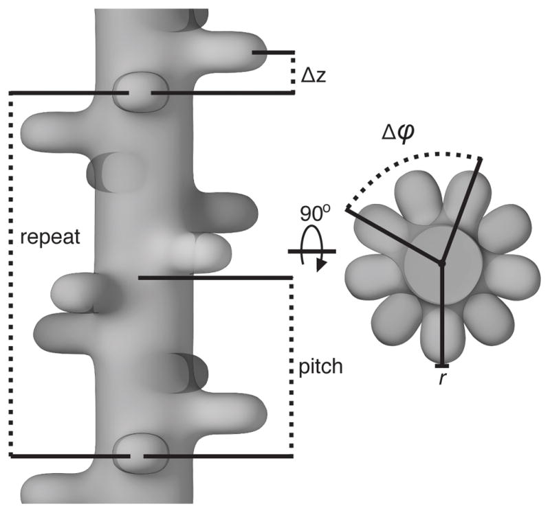
Helical symmetry is defined by the azimuthal rotation angle Δϕ, which is the angle s subunit must be rotated to overlap with its next copy (80° in the example shown), and an axial rise Δz, which is the translation along the axis between subunits. In addition, in IHRSR it is necessary to specify the outer radius of the cylinder that encompasses the filament and beneficial to give the inner radius in the case of tubular filament. Finally, one may consider repeat, which is the distance that a subunit needs to be translated axially to be in exact register with another subunit, and a pitch, which is the distance over which the helix makes a 360° turn. For the case illustrated the repeat is exactly 2 times the pitch (4.5 subunits per pitch; 9 subunits per repeat).

IHRSR was originally implemented by Egelman using scripting capabilities of the single particle software package SPIDER (Egelman, 2010). Later modifications allowed application of essentially the same scheme to multireference 3D alignment, and thus enabled analysis of heterogeneous helical specimens (Wang et al., 2006; Yang et al., 2003). Independent implementations of IHRSR were subsequently undertaken by others. Volkmann re-implemented IHRSR following the original outline and using EMAN and CoAn image processing packages (Lowey et al., 2007). Grigorieff and co-workers utilized the original SPIDER scripts with alterations aimed at taking advantage of some features offered by Frealign (Sachse et al., 2007). In particular, they modified 3D reconstruction step to avoid simplification of the original Egelman procedure. Strictly speaking, application of helical symmetry to the refinement model should be done by including all symmetry related versions of each 2D projection image during 3D reconstruction instead of directly applying helical symmetry to this structure, because the former assures the proper Fourier space weighting of contributing projection data (Penczek, 2010). However, the rise of the TMV symmetry is very small (1.408Å), so the number of symmetry related versions of a projection for the segment size used (774.0Å) would be very large, which in turn would result in excessive calculation times. Thus, the actual 3D reconstruction was done using averages of projection data that have the same projection directions.

Here, we describe a new implementation of IHRSR in SPARX (Hohn et al., 2007) that introduces a number of features aimed at improving the quality of the results and convergence properties of the algorithm. We built on the experience gained from over a decade of use of the original version available as a SPIDER script, but on the other hand we modernized the implementation by taking advantage of the improved scripting capabilities of SPARX and recent advances in cryo-EM data processing. We also put forward a novel analytical tool, the helical Principal Component Analysis (hPCA) for assessing specimen flexibility particularly suitable for sorting out conformational variability of helical assemblies.

2. Helical symmetry in biological objects

Definition of helical symmetry and conventions used in EM

Helical symmetry is given, in cylindrical coordinates, by two parameters: azimuthal rotation per subunit Δϕ and axial subunit translation Δz:

$$f(r,\varphi ,z)=f(r,\varphi +n\mathrm{\Delta }\varphi ,z+n\mathrm{\Delta }z),n=\pm 1,\pm 2,\rightleftharpoons$$ (1)

where $r=\sqrt{x^2+y^2}$ (Fig. 1). In addition, one may consider the helical repeat, which is the distance that a subunit needs to be translated axially to be in exact register with another subunit. The value of the repeat is not relevant for the real-space processing of helical specimen, as (1) it varies dramatically with a small change in helical symmetry parameters Δϕ and Δz and (2) its value can exceed by far what can be reasonably imaged in electron microscope and processed in a computer. For example, TMV has 49.02 subunits in three turns, with an axial rise of 1.408Å per subunit (Stubbs and Makowski, 1982). The helical repeat would therefore be 50*49.02=2,451 subunits, or a distance of 3,451Å. The helical symmetry axis is always assumed to coincide with the z axis of the coordinate system¹. In addition, helical objects can have one of two point group symmetries: cyclic (Cn) or dyadic (Dn). For Cn, the symmetry axis coincides with the helical symmetry axis (z); for Dn the main axis is also z while the additional 180° symmetry axis is selected to coincide with y′ axis of the 2D coordinate system of projection data.

In EM the filaments are prepared on a supporting grid and imaged in direction of the electron beam perpendicular to the grid plane (unless tilt is used). When filaments are windowed and segmented, they are typically oriented such that the filament axis coincides with the y′-axis of the 2D system of coordinates of projection data (z axis of 3D coordinate system projects to become y′ axis of 2D projections). If we ignore possible out-of-plane tilt of filaments, a set of filament segments windowed using equal steps along the filament axis will constitute a set of uniformly distributed single axis tilt projections oriented perpendicularly to the helical symmetry axis of the filament in 3D space, i.e., their projection directions are oriented perpendicular to the z-axis (Fig. 2). Such a set is called orthoaxial (Vainshtein and Penczek, 2008). Given sufficient number of randomly oriented filaments, the projection directions will form a half-circle in the x-y plane and it follows that such a set is sufficient to fully reconstruct a 3D mass distribution of the filament to the resolution limited only by the signal-to-noise ratio (SNR) and quality of the data. The projections from a single filament, on the other hand, can only yield a number of distinctly different projections that is determined by the number of subunits in the repeat. For an integer number of subunits per turn, or for a small number of turns in the helical repeat, a limited number of different projections will be obtained. This manifests itself in the Fourier-Bessel formalism as Bessel overlap (more than one Bessel function on the same layer line) at a limited resolution.

Figure 2. Geometrical relations between micrograph 2D data, the 3D helical filament and its 2D projections.

(A) Sample micrograph of a mixture of actin filaments with and without bound myosin. Scale bar 100 nm. (B) Windowed out filament segment whose dimensions are x′, y′; segments are normally squares. For each segment, one has to establish its in-plane translation and in-plane angle ψ with respect to common reference of a 3D map of the specimen. (C) Azimuthal orientation of the segment is given by angle ϕ which together with in-plane orientation parameters is established by a 3D projection alignment procedure. Here we show planar projection image (B), in which case projection directions are perpendicular to the helical symmetry axis z, in which case they are called orthoaxial (θ = 90°). Presence of out-of-plane tilt of filaments requires considering non-orthoxial projection direction (θ ≠ 90°).

An orthoaxial set of projections (θ = 90°) is also known as single-axis tilt series. Unlike in electron tomography where a wedge of projection directions is missing (Penczek and Frank, 2006), the set of projections from helical structures, in the limit of many random filaments, is complete, i.e., the available angular range of 0° ≤ ϕ < 180° is sufficient for an artifact-free inversion of a projection problem with the resolution limit imposed by the number of projections, quality of EM projection data (its SNR), and finally distribution of defocus values used for imaging. A 3D reconstruction performed using orthoaxial projections will have an extremely uneven distribution of spectral SNR (SSNR) (high along z axis, low on peripheries of x-y planes of reciprocal space), but at the same time artifacts due to the geometry of the reconstruction process are minimized (Penczek and Frank, 2006).

Unique subunit of a helical filament and geometrical relations of its projections

In the absence of point group symmetries, a unique subunit fully sufficient to generate an arbitrarily long filament is a disk with a height Δz and limited by maximum radius r_max. For Cn point group symmetry the unique subunit is a “pie”, i.e., the fragment of a disk limited by range of angle ϕ between 0° and 360°/n, height Δz, and maximum radius r_max. For Dn point group symmetry the unique subunit is a fragment of a disk limited by range of angle ϕ between 0° and 360°/n, height Δz/2 and maximum radius r_max

Helical structure determination with IHRSR usually begins with the assumption that out-of-plane tilt can be ignored. This not only accelerates the calculations, but makes IHRSR process more robust and allows for a quick estimation of approximate helical symmetry parameters. In order to assure proper convergence, one has to carefully consider angular properties of projection directions of an orthoaxial set. Projections with directions θ = 90° and 180° ≤ ϕ < 360° are mirrored (in plane) versions of the first set, i.e., Prj(θ = 90°, ϕ) = Prj_mirror (θ = 90°, ϕ + 180°) and since the projection alignment algorithm employed in SPARX checks for mirror orientations of data, only azimuthal range 0° ≤ ϕ < 180° is considered here. In the presence of point group symmetries, the unique range of azimuthal angle for orthoaxial projections narrows and is:

1. Cn

   • 1.1n even: ϕ ∈ [0,360/n)
   • 1.2n odd: ϕ ∈ [0,360/2n)

2. Dn

   • 2.1n even: ϕ ∈ [0,360/2n)
   • 2.2n odd: ϕ ∈ [0,360/\4n).

(for Cn-even symmetry, orthoaxial projections have additional 2-fold symmetry about y axis, but this cannot be easily taken advantage of).

Given that the SPARX implementation of IHRSR restricts angles of template projections to the unique ranges given above (including mirror transformation), in order to generate a valid 3D reconstruction in case of point group symmetry one needs symmetrization rules for generating the full range of projections (i.e., the symmetry related versions of projection directions). For projection directions with θ ≠ 90° it is sufficient to apply n times the point group symmetry operator to have the necessary information. For orthoaxial projections, the rules are more complex and in addition depend on n being either odd or even (see Supplemental Information).

3. Principle of Iterative Helical Real Space Refinement

To initiate IHRSR it is required to have a good approximation of helical symmetry parameters Δϕ and Δz, as obtained from indexing of the diffraction pattern of the filament or from measuring the molecular mass per unit length with STEM ((Wall and Hainfeld, 1986). Next, one has to specify the radius r_max of the cylinder encompassing the filament and for hollow tubes in addition the internal radius. Finally, one needs an initial 3D object. In order to avoid a bias, a preference is given to a cylinder with radius r_max filled with low-pass filtered Gaussian noise, which is sufficient for the method to converge as long as approximate initial symmetry is known (Egelman, 2007). This initialization method has additional advantage of enforcing proper in-plane orientation of windowed segments beginning from the first iteration.

IHRSR proceeds by alternating between 3D projection matching whose goal is to establish orientation parameters of EM projection data (Eulerian angles and in-plane translations) (Penczek et al., 1994) and a 3D reconstruction yielding an update of the helical structure (Fig. 3). The 3D reconstruction algorithm does not include helical symmetrization; this is done independently using current values of helical symmetry parameters. Optionally, symmetrization is preceded by a search for corrected helical symmetry parameters (Egelman, 2010). Typically, during the first few iterations a straightforward projection matching would be executed with additional enforcement of initially assumed helical symmetry parameters. During subsequent iterations, the helical parameters would be adjusted: given a new update of the reconstructed but not symmetrized structure, different combinations of helical parameters would be tried by varying slightly the previously determined ones. As a criterion of the symmetry fit we selected the L2-norm of the symmetrized structure (sum of squared voxel values) whose maximization can be shown to be equivalent to the minimization of the variance of the reconstructed structure (Penczek et al., 1992), with the former much easier to calculate. The symmetry parameters that maximize the L2 norm of the symmetrized structure would be accepted as the improved ones for the next iteration.

Figure 3. Flowchart of IHRSR.

The iterative process of real space helical structure determination is initiated by providing a template 3D structure, for example a cylinder filled with Gaussian noise, and a guess for helical symmetry parameters. The process alternates between 3D projection matching, during which EM projection data is compared with reprojections of template structure using a correlation technique, reprojections of the template structures, and a 3D reconstruction yielding an update of the helical structure. During first few iterations, the initial symmetry is enforced, while subsequently the symmetry parameters are updated. Optionally, both steps of symmetry search and symmetrization of the structure can be omitted.

Barring unlikely mistakes, the orthoaxial distribution of projection directions of a helical object should be uniform, therefore simplifying somewhat the methodology. The helical symmetry is applied directly to the 3D map, as emerged from the 3D reconstruction step. This simplification not only results in a very significant speedup of calculations, but also makes it possible to correct for a possible change of initially assumed helical symmetry parameters. This is done using a brute force approach, i.e., various combinations of Δϕ and Δz symmetry parameters are used to symmetrize the reconstructed map and the set corresponding to the symmetrized structure that has largest squared norm is chosen. Thus, with possible exception of the first few iterations, the procedure updates both orientation parameters of the projection data and helical symmetry parameters at each iteration.

The convergence of the iterative process is monitored by examining (1) angular assignments of projection data, which are expected to settle, (2) the azimuthal distribution of projection directions (i.e., values of ϕ angle), which is expected to be uniform within the range 0° ≤ ϕ < 180° (or a subrange, if point group symmetry is present), and (3) the helical symmetry parameters, which should adopt ultimate values and cease to change. While under normal circumstances IHRSR will “converge” in a finite number of iterations fulfilling the three requirements listed above, there is no guarantee that the 3D structure will correspond to true structure of the biological specimen imaged. First, if the initial guess of helical symmetry parameters is too distant from the correct ones the procedure described will fail to determine the proper values. How good this guess has to be depends on many factors, including the effective distance from alternate symmetries, the number of EM projection images used, the quality of the data, and so on. Second, the helical object studied may have intrinsic ambiguities in helical symmetry, i.e., within the resolution limit of the data the power spectrum of helical structure (i.e., the layer line pattern) may correspond to a number of quite different sets of helical symmetry parameters (Egelman, 2010). Finally, even if the procedure finds the correct helical symmetry (or the symmetry was known in advance and simply enforced during the iterative process) and “converged” in the sense of three criteria given above, there is no guarantee that the solution found is optimal in the sense of corresponding to the highest possible resolution that can be obtained for a given data set. The reason is that the optimization scheme adopted in IHRSR is based on a single particle 3D projection alignment scheme that corresponds to a simplistic downhill minimizer. Therefore, reaching the global optimum cannot be guaranteed (Yang et al., 2005). Thus, while IHRSR will find a 3D map of a helical object, it cannot be guaranteed that the structure will be correct or even the best possible one for a given EM data set. However, owing to high degree of averaging and regularization properties of helical symmetry imposed, the procedure is extremely robust and capable of delivering structures in cases when other approaches may fail.

4. IHRSR implementation in SPARX

3D reconstruction and reprojections computed within rectangular prism

For filamentous specimens, electron micrographs contain projection images that are typically very long, i.e., their lengths exceed the rise of the helix by a large margin. The procedure developed for IHRSR requires that the filament projection images are windowed into square units termed segments. Each segment is large enough to contain a length of the imaged filament that corresponds to at least a few copies of the subunit. In addition, in order to maximize the amount of data used for 3D reconstruction and alignment, the adjacent segments are allowed to extensively overlap with the y-axis translation between them slightly larger than the rise (not 90% of the window size, as often erroneously assumed). The windowing is done interactively using a dedicated graphical user interface program, such as the e2helixboxer.py utility of EMAN2 (http://blake.bcm.edu/emanwiki/EMAN2/Programs/e2helixboxer).

As IHRSR implementations rely on computational methodology inherited from single particle applications, both 3D reconstruction and reprojection algorithms require the data to be placed within a cubic volume, i.e., all three dimensions (x, y, and z) to be the same extent. Cubic geometry does not however match the geometry of biological filaments, which fit into a rectangular prism with a length (z dimension) significantly different from the dimensions of the x-y base. A primary consideration is the relation between the length of filament 2D segments used for windowing, the diameter of the cylinder encompassing the filament, the rise of the subunit, and expected flexibility (disorder) of the filament. While longer segments provide more signal, and thus reduce the alignment error and improve the resolution, the imperfect ordering of the helical specimen dictates a tradeoff as shorter segments are more likely to be more coherent (see Fig. 6.4 in (Egelman, 2010)). In addition, for specimens with large rise, the segment has to be sufficiently long to accommodate a sufficient number of rise units, so that artifacts of 3D reconstruction and symmetrization can be minimized. For example, for myosin-decorated actin filaments considered in subsequent sections, the rise is Δz = 27.6Å and the segment was selected as 405.0Å, thus the reconstructed map comprised 14.7 rise units. As the diameter of the specimen is only about 200.0Å, the structure is preferably contained within a rectangular prism that is at least twice as long as broad. At the same time, for helical tubes the relations are often reversed. In case of TMV helix, its rise is 1.408Å, but the diameter is 180Å. It follows that to have the same number of rise units as for the myosin-decorated actin filaments, the height of the rectangular prism should be nine times smaller than its width! Thus, if the projection/reconstruction code could handle non-cubic volumes, one would expect significant reduction in computer memory requirements and in time of calculations.

Figure 6. Calculation of the 3D standard deviation map using hPCA.

(A) 3D map of an actin filament decorated with myosin obtained after 30 iterations of IHRSR without application of symmetry during the refinement. (B) 3D map separated into disks with a height of Δz. Outermost disks were discarded. (C) Disks rotated by integer amounts of Δϕ to match the orientation of the central disk. Differences between the disks are obvious for a region corresponding to parts of the converter domain of myosin (marked by arrow). (D) 3D map of myosin overlaid with a shell corresponding to significance level of α = 5% (1.96 * SD). The map shown corresponds to the marked region in (A) but was obtained after application of helical symmetry. The arrow marks the same region of the converter domain as in (C).

In the last decade, reconstruction algorithms routinely used in most single particle packages gravitated towards direct Fourier inversion algorithms (Penczek, 2010). These algorithms are based on the Central Section Theorem, according to which a Fourier transform of a 2D projection of a 3D object is a 2D central section of the 3D Fourier transform of this object and is oriented normal to the projection vector (Bracewell, 1956). A direct consequence is a possibility to accomplish 3D reconstruction by “insertion” of Fourier transforms of 2D projections into a 3D Fourier volume using some form of interpolation. As long as the interpolation scheme used is simple, the method tends to be very fast and naturally accommodates CTF correction. Finally, typically large number of projection images and oversampling of Fourier space during interpolation mitigates reconstruction artifacts that otherwise might be caused by the unsophisticated reciprocal space interpolation schemes employed. In particular, the SPARX implementation is based on a nearest neighbor (NN) reciprocal space interpolation with 4x (optionally 2x) padding of input projections to reduce interpolation errors. The CTF correction is integrated with the reconstruction step via a Wiener filter type summation of Fourier components (with possible addition of a regularizing constant (Penczek, 2010)), which schematically is written as (Zhang et al., 2008):

$$D=\frac{{\displaystyle \sum _n}{\mathit{CTF}}_n{\mathit{SSNR}}_n{G}_n}{{\displaystyle \sum _n}{\mathit{CTF}}_n^2{\mathit{SSNR}}_n+1}$$ (2)

After all projection data is processed, additional per-voxel reciprocal space weighting is applied to account for possible gaps in coverage of the 3D Fourier volume (Zhang et al., 2008). Finally, 3D inverse FFT and windowing out the relevant part of real-space volume complete the 3D reconstruction process.

In the SPARX implementation of IHRSR we require that windowed segments are squares. While it would be possible to have rectangular segments, we decided disadvantages of such a solution would outweigh possible gains. A smaller window size decreases the accuracy of the CTF correction, both during 2D alignment (projection matching) and 3D reconstruction. The 2D alignment code generally requires square images, as otherwise the rotation of images becomes problematic. Finally, windowed segments should be sufficiently large to accommodate translations of filaments during 2D alignment, which would put a limit on how “tightly” filaments could be windowed. Thus, the solution adopted is to have a 3D reconstruction code that implicitly windows the relevant rectangular part of the square 2D projection image and places its backprojection into a rectangular prism 3D volume. Conversely, the 3D→2D projection code places the result of rectangular prism volume projection in a square projection window.

In the implementation in SPARX, which accommodates the use of arbitrary combinations of x-y-z sizes in the 3D reconstruction algorithm, we assumed that 2D projection images are squares, i.e., x′ = y′. We modified the reciprocal space interpolation scheme employed to implicitly window the relevant part of the projection image. We took advantage of the fact that decimation in one space corresponds to windowing of the central part of the signal in transformed space. Here, during mapping of 2D Fourier pixels into 3D Fourier volume we adjusted steps on the 2D grid by the ratio of modified dimensions ( $\frac{x^{\prime }}{x}>1$ for volumes with narrow x-y base, or $\frac{z^{\prime }}{z}>1$ for volumes with reduced height), which corresponds to using only the central rectangular real-space portion of the 2D projection image. As the 2D locations are generally off Cartesian grid, we used bi-linear Fourier space interpolation to find the associated values and the NN interpolation to assign them to voxels on a central section Cartesian grid in 3D (whose orientation is perpendicular to the projection direction).

Reprojections of a 3D structure are computed in SPARX using the highly accurate and efficient reverse gridding technique (a method that belongs to a family of non-uniform Fourier transforms) (Penczek et al., 2004). Briefly, a 3D volume is padded with zeroes in real space to twice its size, a 2D central section perpendicular to projection direction is extracted using convolution with Kaiser-Bessel (K-B) kernel (we use box 6×6×6 voxels), its 2D inverse FT is computed, effect of convolution is removed by a real-space division by the FT of the K-B kernel (a sinh function) and the relevant part is windowed out. In order to modify the algorithm such that it can project content of volumes with arbitrary combinations of x-y-z dimensions into 2D square projection images, i.e., x′ = y′, max(x,y,z) = x′ = y′, we took advantage of the fact that oversampling in one space correspond to padding with zeros of the central part of the signal in the reciprocal space. As in the gridding technique the convolution step naturally extracts the reciprocal space voxel values at arbitrary locations, thus making the implementation of the mixed dimensions reprojection algorithm straightforward.

The modified code for backprojection and reprojection operations can handle data using any combination of x-y-z dimensions. The main savings are in the computer memory required. For example, using a volume size of 220×220×400 voxels instead of 400×400×400 voxels reduces memory requirement during the reconstruction step from ~4GB to 1.2GB (assuming 2x padding and taking into account that the program needs two volumes to perform reconstruction, one for the numerator and the other for denominator of Eq.1). Some increase in the speed of 3D reconstruction step is also notable, for example 3D reconstruction using 10,000 images that are 400×400 pixels takes, using 8 CPUs, 533s if the target volume size is 400×400×400 voxels, but only 185s if the target volume size is 220×220×400 voxels. Thus, the speed up is ~2.9 times, which roughly corresponds to the ratio of the size of target volumes.

3D projection alignment settings that strictly follow the helical symmetry

The 3D projection alignment is based on 2D correlation comparisons between EM projection data and template reprojections of a 3D object. In SPARX, this is accomplished using a methodology based on resampling to polar coordinates (Joyeux and Penczek, 2002). Briefly, both images are resampled to polar coordinates with respect to the center of the image frame. 1D FFTs of points on each concentric ring are computed and the inverse FFT of the sum of their product yields a 1D rotational cross-correlation function (ccf), whose maximum location corresponds to the angle between the two images. The translation of a projection image is obtained by repeatedly applying this algorithm, but with varying origins of aligned image. The overall maximum of the 1D ccfs for all origins yields both the angle and the in-plane translation (see Fig. 1 in (Joyeux and Penczek, 2002)). It follows that the translation search has discrete step sizes and is limited in x′ and y′ (though both step size and range can be different for the two directions). While the preference is usually given to an integer number of pixel-sized steps, SPARX implementation of the algorithm accommodates arbitrary combinations of parameters.

As helical specimens are windowed such that their long axis is aligned with the y′ axis of the segment, the parameters of the translational search in x′ direction (perpendicular to the symmetry axis) are established naturally. The x′-range should correspond to the error in centering of the segments and the step size should match the expected resolution (usually 1.0 or 0.5 pixels is sufficient). x′-axis pre-centering is recommended for IHRSR as it reduces the range of x′-axis translation search and thus the time of calculation and number of iterations required for convergence. In SPARX, the y′-axis search range is set to correspond to the current value of the rise Δz, which ensures that the entire range of azimuthal angle ϕ is also covered, as elaborated above. Thus, the user specifies an integer number of steps and the program computes the step size based on current value of the rise Δz. In this way, the program naturally accommodates the fact that the helical symmetry parameters may change from one iteration to another. It also follows that restricting the y′-axis search range to that of the helical rise dictates that the optimum overlap between adjacent segments windowed from a filament should be slightly larger than the rise.

In order to avoid multiple interpolations of the input EM projection data, the images are not modified by IHRSR, i.e., they are neither shifted nor rotated. Instead, after each iteration the program will update the current orientation parameters, including Eulerian angles needed for 3D reconstruction, by combining those stored in the image header with the updates resulting from the current iteration. However, these running updates mean that the origin of the EM projection image can potentially “drift away” from the permitted y-range, which is the rise Δz. Therefore, we implemented a procedure which after each iteration maps the orientation parameters back into the permissible range, and which includes restrictions on out-of-plane tilt (angle θ).

An additional feature of the IHRSR implementation in SPARX is an optional “local” angular search, i.e., search for Eulerian angles of a projection image that is only done within a specified angular neighborhood of its previously determined angular direction. This feature is used in high-resolution refinements to prevent projection data from drifting away to false locations and to reduce the time of calculations.

Graphical user interface (GUI) for IHRSR in SPARX

The successful execution of IHRSR requires setting of a large number of parameters, of which only a subset is discussed here. The additional flexibility offered by the SPARX implementation requires additional parameters, some of which will only be used rarely. While an exhaustive documentation is provided (see http://sparx-em.org/sparxwiki/sxihrsr), selecting specific parameters that are required to activate the program can be daunting. We addressed this issue by developing a “graphical command editor” in form of a GUI that allows the user to set values of parameters and to enter names of files and directories (Fig. 4). While it is possible to activate IHRSR directly from the GUI, a recommended alternative is to use the GUI to generate a SPARX command line that is stored in a file, thus is archived, and can be subsequently used to execute IHRSR on a remote computer system. Finally, all parameters can be stored in a format readable by the GUI, so they can be read in subsequent sessions, modified, and thus help the user to execute multiple runs of IHRSR for the purpose of exploring the full potential of the data set.

Figure 4. IHRSR SPARX GUI command editor.

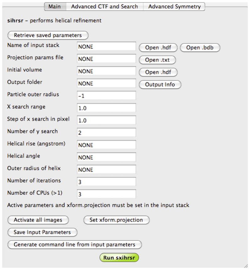
GUI facilitates entering of parameters that specify the helical structure determination process in SPARX. In addition to helical symmetry parameters, one can specify search ranges, radius of the 3D structure, and various advanced settings. The parameters can be saved for future use. The primary function of GUI is to generate the command line and to store it to a disk file. However, in the case when data are processed on a cluster that the user has a direct access to, it is also possible to activate IHRSR directly from the GUI.

To simplify the interaction with IHRSR we subdivided the GUI into three screens. The Main screen contains parameters that are necessary for the program to operate properly and includes names of data files and output folder, helical symmetry parameters, number of iterations, and number of CPUs available for the MPI processing. The Advanced CTF and Search screen contains parameters related to CTF correction and to advanced orientation search options, for example range for out-of-plane tilt. Finally, Advanced Symmetry screen includes additional parameters that govern search for helical symmetry in IHRSR.

6. Analysis of specimen heterogeneity

Helical PCA

We demonstrated previously that resampling techniques applied to single particle cryo-EM data sets yield information that can be used to identify multiple conformational states of the specimen present in the sample (Penczek et al., 2011; Zhang et al., 2008). Indeed, in the newly developed codimensional PCA (CD-PCA), 2D projection images are sampled independently within angular regions (strata) such that the overall distribution of all selected projections is approximately uniform. After computing large numbers of resampled volumes from repeatedly selected projection subsets, the resampled maps (1) are used to compute the 3D variance field and (2) are subjected to PCA to yield eigenvectors of the system. We term the latter the eigenvolumes. A small number of thus obtained dominating eigenvolumes are reprojected in directions of input EM projection data and the inner products between pairs of these images yield factorial coordinates of 2D data within a common framework of the analyzed 3D structure. Finally, the factorial coordinates undergo cluster analysis and based on the resulting class assignments for projection data, the 3D structures of conformers are computed (Penczek et al., 2011).

Application of codimensional PCA to helical filaments is straightforward. In fact, as the distribution of angular directions is always nearly uniform (θ close to 90°, ϕ approximately uniform in the range from 0° to 180°), the stratified resampling is very efficient. Furthermore, as the reconstructed and helical-symmetrized 3D map can be thought of as a stack of identical disks each ΔzÅ high (and rotated by nΔϕ, which for the purpose of what is considered here is irrelevant), it is sufficient to extract from each resampled 3D map one such disk and apply PCA analysis to a set of such disks. This yields a small number of dominating eigenvectors (further referred to as eigendisks). After restacking of appropriately rotated versions of a given eigendisk, we obtain an eigenhelix. A set of eigenhelices is used to compute factorial coordinates of projection data in a common 3D framework of the given helical filament. After clustering of factorial coordinates we can compute 3D structures of plausible helical conformers and split the dataset accordingly. We refer to this modified version of the CD-PCA method as helical CD-PCA (hCD-PCA).

The helical geometry of filaments considered here leads to a much simpler, accurate, and computationally more efficient procedure termed helical PCA (hPCA) (Fig. 5) that yields results superior to those obtained using hCD-PCA. Indeed, let us consider a 3D map computed using orientation parameters derived from IHRSR refinement, including helical symmetrization, but that itself was not symmetrized (Fig. 6A). Such a map would be nearly helical, as the symmetry was enforced during IHRSR iterations, but since the symmetry was not applied, each unique disk (non-overlapped region of each segment) would constitute a slightly different version of the “average” disk that would result from symmetrization. Therefore, it is straightforward to extract all disks from the reconstructed map (with possible exception of those located on either extreme end, as these are artifactual due to geometry of the system and the alignment procedure itself) (Fig. 6B), rotate them by −nΔϕ, and apply statistical analysis to the thus obtained set (Fig. 6C). In order to avoid interpolation artifacts on the edges of disks, we recommend adjusting the pixel size of the data (by interpolation of the 2D images) such that the height of a unique disk (the rise) approximately coincides with an integer number of voxels. It can be shown that for a change of the original pixel size within 1%, the error of approximation will be all but negligible. A Python program that computes pixel adjustment factor given original pixel size, rise, and segment length is included in the Supplemental Material. Finally, it is worth pointing out that hPCA can be considered a form of oversampling of the projection data. Indeed, each segment contains multiple instances of projections of unique lengths of the helix and in addition IHRSR requires the segments to overlap significantly. It follows that within the reconstructed disks contributions from helices that differ in conformation will mix in different proportions. If helical symmetry is not enforced, these disks will differ in a manner similar to the way structures obtained from resampled subsets of projections differ in resampling-based analysis of asymmetric structures (as it has been implemented for CD-PCA or hCD-PCA).

Figure 5. The sequence of steps constituting helical PCA.

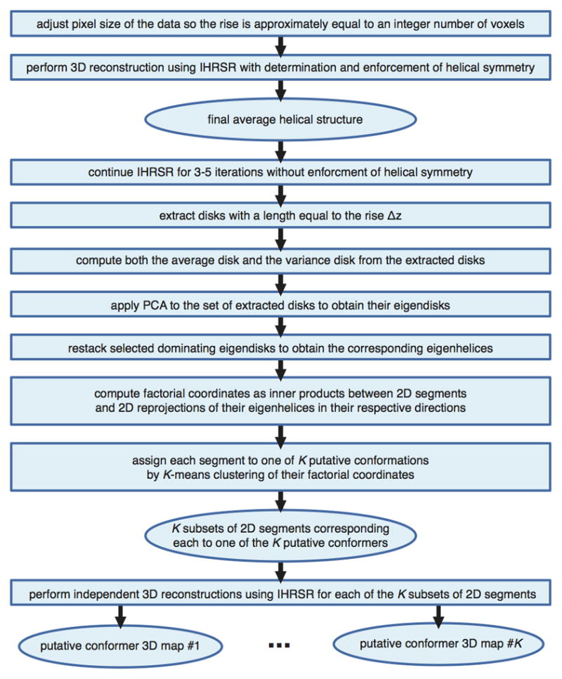
The analysis relies on a structure of a helical specimen using IHRSR with subsequent refinement without enforcement of helical symmetry. This makes it possible to extract a number of disks with length equal to rise, which then are subjected to PCA analysis. The resulting eigendisks are restacked yielding eigenhelices whose reprojections are used to compute factorial of input 2D EM projection images. The clustering of factorial coordinates with subsequent 3D reconstruction of resulting subgroups yields structures of putative conformers.

Nevertheless, hPCA has two major advantages over the resampling approach used in CD-PCA and hCD-PCA: (1) it is possible to compute both the accurate average disk and its standard deviation map, with the latter volume equating to the error of the reconstruction. (2) It is readily possible to apply PCA to the set of disks. Since the number of disks is necessarily small (approximately equal to nz · p/Δz − 2, where nz is the length of the reconstructed filament in pixels and p is pixel size in Å) so is the number of eigendisks that can be obtained. This is however of limited practical importance, as in our analysis we are primarily constrained by the resolution and generally interested only in large-scale variability of the structure. Therefore, we are only interested in a small number of dominating eigendisks. Given these eigendisks, we proceed as described earlier in case of h-CD-PCA: eigendisks are restacked, factorial coordinates of projection data calculated, subjected to clustering leading to 3D structures of plausible conformers. In addition, the accurate standard deviation map obtained using hPCA allows plotting a surface corresponding to a selected significance level of the filament map, i.e., the 3D region within which a surface of the structure could be located at α significance level. Standard deviation of EM map voxel values also makes it possible to carry out a proper docking of X-ray crystallographic segments that accounts of nonuniform error and/or flexibility of the imaged structure.

The hPCA approach described above is marred by one practical difficulty, namely that the noise component in extracted disks is correlated. This follows from the fact that the template 3D structure used in IHRSR is helically symmetrized. Taking into account that this template is a stack of identical (in principle, ignoring interpolation errors) unique segments of the filament, during 2D alignment each band within 2D EM projection of the filament is aligned to the reprojection of the same unique disk (it makes no difference that segments are rotated by multiplicity of Δϕ). It follows each band is presented with a template that is a projection of the same 3D disk. In effect, the noise in each disk, while independent between density bands in the projection data, becomes correlated by virtue of being aligned to the same template.

There are various possibilities for how to deal with the correlated noise problem. (1) The simplest approach is to take advantage of the fact that the degree of induced correlation is very high and in the PCA results the artifact always manifests itself as the most prominent first eigendisk, whose eigenvalue is much larger than those of remaining, meaningful eigendisks. Armed with this observation, we can simply ignore the first meaningless eigendisk. (2) Alternatively, it is possible to follow IHRSR converged result obtained with symmetrization by additional iterations without imposing helical symmetry until convergence is reached again. With a proper choice of projection alignment strategy, it is possible to all but eliminate the induced correlations between noise component in disks. (3) Whenever convergence to a correct solution can be accomplished without imposing helical symmetry, it is recommended to carry out IHRSR refinement without symmetry enforcement during reconstruction, which will result in artifact-free eigenanalysis (see the example below for a proof of principle that a reconstruction without applied helical symmetry can yield the correct 3D structure in a particular case).

Application of hPCA to the analysis of conformational variability of actomyosin

We applied both hCD-PCA and hPCA to a cryo-EM set of myosin-decorated actin projection images (Behrmann et al., in preparation). Briefly, the data set contains approximately 60,000 filament segments images collected on a 200kV microscope at a magnification of 170,000x under minimal dose conditions. Defocus settings ranged from 0.75 μm to 1.5 μm, while image contrast was enhanced by zero-loss filtering with a slit-width of 12 eV. In addition to the low SNR of the projection images, reconstruction was further complicated by the coexistence of actin filaments with at least three different subsets of myosin-decorated actin filaments that differ only slightly in the conformation of myosin. Initial conformational analysis was performed on this data set using hCD-PCA as described above. As the data converges to the correct solution without imposing helical symmetry (Fig. 7), we were able to apply hPCA directly to the disks extracted from the unsymmetrized 3D map of myosin-decorated actin filament to compare results to those previously established using hCD-PCA. Given that the segment length was 404.8Å, Δz = 27.6Å, Δϕ = −166.5°, and pixel size 1.84Å, we were able to extract 12 disks. We first computed a standard deviation map, which clearly demonstrates that a region of myosin corresponding to a flexible hinge region (Dominguez et al., 1998) is not as well resolved as other parts, especially the inner actin filament, of the structure. To further investigate this result and to determine the reason for this observation, we used the asymmetric rise-disks to compute eigendisks. The first, dominating one accounted for the initially observed variability of the flexible hinge region corroborating previous results obtained with hCD-PCA (albeit at a vastly improved resolution compared to the previous results).

Figure 7. Estimation of helical symmetry parameters from unsymmetrized reconstructions.

(A) 3D map of actin-myosin-tropomyosin complexes obtained using the standard IHRSR scheme of alternating projection matching/reconstruction and search for symmetry parameters and symmetrization. The converged helical symmetry parameters were Δz = 27.6Å and Δϕ = −166.5°. (B) 3D map of the same complex obtained using IHRSR without application of helical symmetry. (C) 3D map of complex shown in (B) after application of estimated helical symmetry parameters (see E). The symmetrized volume obtained from the reconstruction without application of helical symmetry closely resembles the structure obtained using the standard IHRSR scheme, though the volume appears to be less well defined. (D) Plot of correlation scores for the helical parameters Δz and Δϕ used to establish helical symmetry of the 3D map obtained without enforcing helical symmetry (shown in B). (E) Top ten ranking pairs of Δz and Δϕ. The highest ranking parameters were Δz = 27.6Å and Δϕ = −166.5°.

It is instructive to compare the results obtained with hPCA with those that were obtained using hCD-PCA (which is based on per-helix resampling instead of per-disk resampling). The main difference is that as elaborated elsewhere (Penczek et al., 2011), the per-voxel variance map computed using resampled volumes is of insufficient resolution to yield useful results. In contrast, the variance map derived from hPCA is obtained at resolution corresponding to that of the original map and as shown here convincingly identifies the main source of variability in myosin as a region belonging to the flexible hinge region (compare Fig. 8A with D). At the same time, the dominating eigendisks for the two respective approaches have similar effects on the average structure though at vastly different resolutions (compare Fig. 8B, C with E, F). Finally, hCD-PCA requires significant computational resources in order to compute sufficient number of resampled volumes and the time of calculations is in the order of hours, even using multi-CPU cluster. In comparison, hPCA only takes a minute or so on a single CPU - time entirely negligible in comparison with any of the steps involved in IHRSR. In addition, it is apparent that the obtained resolution of the variance analysis differs strongly between hCD-PCA and hPCA. While for hCD-PCA the 2D EM images usually need to be downsampled to reduce both CPU and hard-disk needs, hPCA can be performed directly from the unmodified dataset and thus yields a better resolved estimation of variance and more detailed eigenvolumes. Therefore, it can potentially differentiate between closely related conformers that would be masked otherwise in the lower resolution of hCD-PCA.

Figure 8. Comparison of hPCA with hCD-PCA analysis of conformational variability.

(A–C) hPCA results: (A) Average map rebuild from the asymmetric unit disks overlaid with a map representing α = 5% (1.96*SD). (B) Average map shown together with the dominating eigenhelix in black. (C) Structure obtained after subtracting the eigenhelix from the average map. Slight rearrangements in locations corresponding to the known flexible hinge region are marked by arrows. (D–F) - hCD-PCA results: (D) Average map rebuild from the resampled map overlaid with a volume representing the SD at a level comparable to the one shown in A. (E) Average structure shown together with the dominating eigenhelix. (F) Structure obtained after subtracting the eigenhelix from the average structure. Slight rearrangements are visible but difficult to interpret.

7. Conclusions

The implementation of the iterative helical real-space reconstruction (IHRSR) procedure in SPARX addresses some of the issues that could not be properly resolved in the original SPIDER implementation. It also adds new features improving robustness and flexibility of the method. The 3D reconstruction and projection can now be done within a rectangular prism volume, which greatly reduces computer memory requirement and also reduces time of calculations. We rationalized searches for orientation parameters, particularly for translation, which now strictly adheres to the rise of the helix and is adjusted automatically by the program in case helical symmetry parameters change their current values. Similarly, angular search range for orthoaxial projections is now properly selected according to point group symmetry of the helix, if present. This prevents projection data from inconsequentially changing angular assignments between equivalent symmetry related orientations, which in turn could lead to a false conclusion that the process is not converging properly.

The new implementation is parallelized using MPI on a python level, which makes it very efficient on multiprocessing distributed memory clusters. In addition, we parallelized the search for helical symmetry using MPI and made it exhaustive; in the original implementation, to make it computationally manageable, the search for rise was separated from that for the helical azimuthal angle. We also enhanced the code by adding the possibility to restrict the search for the in-plane rotation angle ψ of 2D projection data and also to restrict the search for projection directions (angles (θ, ϕ)) to the vicinity of previously established angular directions. Finally, out-of-plane tilt (θ ≠ 90°) orientation searches and proper Wiener filter-like CTF correction integrated with the reconstruction algorithm were added.

The robustness of the new code was demonstrated in the application to the helical structure determination of actin filaments complexed with myosin and tropomyosin. The structure could only be determined to subnanometer resolution after proper separation of the conformational mixture present in the biological sample (Behrmann et al., in preparation). We also showed that proper convergence can be accomplished without enforcing helical symmetry during the refinement process though achievable resolution is limited in this case.

We proposed a novel analytical tool for analysis of conformational variability of helical assemblies, the helical PCA (hPCA). The method is based on the observation that if the helical symmetrization is not applied, a helical 3D map can be thought of as a stack of semi-independent versions of the basic building block of the protein density, a disk (or a pie, in case of point group symmetry). The height of such disk is equal to the rise of the subunit and due to the way IHRSR is applied, the reconstructed map will contain multiple disks, ten or more, depending on the settings of the analysis (the segment size). These disks, after inverse rotation are subjected to PCA and resulting eigendisks provide informational about conformational variability of the specimen. In the case of actomyosin, we demonstrated that the results of hPCA agree with those of the computationally more demanding hCD-PCA analysis and are in fact superior to them due to the increased resolution and the well-resolved standard deviation map. This map could potentially be used to aid with flexible fitting approaches to model pseudo-atomic maps of the assemblies studied.

As hPCA can be executed rapidly, within a fraction of time required by resampling methods, and it also yields high-resolution results, it could conceivably be integrated within the IHRSR scheme. A possible application is to improve convergence properties of IHRSR by estimating non-uniformity of the variance in the reconstructed helix and accounting for it during iterations of IHRSR.

While the current implementation of IHRSR is a major improvement over the decade old original implementation, not all possible modifications have been added, yet. For example, the method would gain if one could trade, during 3D projection alignment, angular range for translational range. Currently, we always consider full angular range and the translational search is restricted to one rise. For helices whose rise is on the order of the pixel size used (as for TMV), the accuracy of the results becomes limited by the step size of translational search and which becomes a fraction of a pixel. In such cases it would be preferential to use a subrange of angular search and have multiplicity of rises used for translational search range.

Finally, it is easy to notice that the method does not utilize the fact that aligned windows originate from a 3D object whose geometry is known very accurately once the helical symmetry becomes established. In principle, given one segment and its Eulerian angles for a perfectly rigid helix one could easily compute Eulerian angles for segments extracted from the same projection image of the same filament. One could use the fact that the segments are not independent in a version of IHRSR that would employ “cooperative refinement”, i.e., orientation parameters of segments emerging from the same filament would be controlled for consistency based on helical symmetry parameters and location of the segment within the filament. Such a modification would increase robustness of IHRSR roughly proportionally to the number of orientation-related segments.

References

- Arnal I, Metoz F, DeBonis S, Wade RH. Three-dimensional structure of functional motor proteins on microtubules. Current Biology. 1996;6:1265–1270. doi: 10.1016/s0960-9822(02)70712-4. [DOI] [PubMed] [Google Scholar]
- Baker ML, Zhang J, Ludtke SJ, Chiu W. Cryo-EM of macromolecular assemblies at near-atomic resolution. Nat Protoc. 2010;5:1697–1708. doi: 10.1038/nprot.2010.126. [DOI] [PMC free article] [PubMed] [Google Scholar]
- Bracewell RN. Strip integration in radio astronomy. Austr J Phys. 1956;9:198–217. [Google Scholar]
- Diaz R, Rice WJ, Stokes DL. Fourier-Bessel reconstruction of helical assemblies. Methods Enzymol. 2010;482:131–165. doi: 10.1016/S0076-6879(10)82005-1. [DOI] [PMC free article] [PubMed] [Google Scholar]
- Dominguez R, Freyzon Y, Trybus KM, Cohen C. Crystal structure of a vertebrate smooth muscle myosin motor domain and its complex with the essential light chain: visualization of the pre-power stroke state. Cell. 1998;94:559–571. doi: 10.1016/s0092-8674(00)81598-6. [DOI] [PubMed] [Google Scholar]
- Egelman E. An algorithm for straightening images of curved filamentous structures. Ultramicroscopy. 1986;19:367–374. doi: 10.1016/0304-3991(86)90096-3. [DOI] [PubMed] [Google Scholar]
- Egelman EH. A robust algorithm for the reconstruction of helical filaments using single-particle methods. Ultramicroscopy. 2000;85:225–234. doi: 10.1016/s0304-3991(00)00062-0. [DOI] [PubMed] [Google Scholar]
- Egelman EH. The iterative helical real space reconstruction method: surmounting the problems posed by real polymers. Journal of Structural Biology. 2007;157:83–94. doi: 10.1016/j.jsb.2006.05.015. [DOI] [PubMed] [Google Scholar]
- Egelman EH. Reconstruction of helical filaments and tubes. Methods Enzymol. 2010;482:167–183. doi: 10.1016/S0076-6879(10)82006-3. [DOI] [PMC free article] [PubMed] [Google Scholar]
- Egelman EH, Stasiak A. Structure of helical RecA-DNA complexes. II. Local conformational changes visualized in bundles of RecA-ATP gamma S filaments. Journal of Molecular Biology. 1988;200:329–349. doi: 10.1016/0022-2836(88)90245-8. [DOI] [PubMed] [Google Scholar]
- Egelman EH, Francis N, DeRosier DJ. F-actin is a helix with a random variable twist. Nature. 1982;298:131–135. doi: 10.1038/298131a0. [DOI] [PubMed] [Google Scholar]
- Fujii T, Kato T, Namba K. Specific arrangement of alpha-helical coiled coils in the core domain of the bacterial flagellar hook for the universal joint function. Structure. 2009;17:1485–1493. doi: 10.1016/j.str.2009.08.017. [DOI] [PubMed] [Google Scholar]
- Hohn M, Tang G, Goodyear G, Baldwin PR, Huang Z, Penczek PA, Yang C, Glaeser RM, Adams PD, Ludtke SJ. SPARX, a new environment for cryo-EM image processing. Journal of Structural Biology. 2007;157:47–55. doi: 10.1016/j.jsb.2006.07.003. [DOI] [PubMed] [Google Scholar]
- Hui MP, Galkin VE, Yu X, Stasiak AZ, Stasiak A, Waldor MK, Egelman EH. ParA2, a Vibrio cholerae chromosome partitioning protein, forms left-handed helical filaments on DNA. Proc Natl Acad Sci U S A. 2010;107:4590–4595. doi: 10.1073/pnas.0913060107. [DOI] [PMC free article] [PubMed] [Google Scholar]
- Jeng TW, Crowther RA, Stubbs G, Chiu W. Visualization of alpha-helices in tobacco mosaic virus by cryo- electron microscopy. Journal of Molecular Biology. 1989;205:251–257. doi: 10.1016/0022-2836(89)90379-3. [DOI] [PubMed] [Google Scholar]
- Joyeux L, Penczek PA. Efficiency of 2D alignment methods. Ultramicroscopy. 2002;92:33–46. doi: 10.1016/s0304-3991(01)00154-1. [DOI] [PubMed] [Google Scholar]
- Klug A, Crick FH, Wyckoff HW. Diffraction by helical structures. Acta Crystallogr. 1958;11:199–213. [Google Scholar]
- Lowey S, Saraswat LD, Liu H, Volkmann N, Hanein D. Evidence for an interaction between the SH3 domain and the N-terminal extension of the essential light chain in class II myosins. Journal of Molecular Biology. 2007;371:902–913. doi: 10.1016/j.jmb.2007.05.080. [DOI] [PMC free article] [PubMed] [Google Scholar]
- Makhov AM, Sen A, Yu X, Simon MN, Griffith JD, Egelman EH. The bipolar filaments formed by herpes simplex virus type 1 SSB/recombination protein (ICP8) suggest a mechanism for DNA annealing. J Mol Biol. 2009;386:273–279. doi: 10.1016/j.jmb.2008.12.059. [DOI] [PMC free article] [PubMed] [Google Scholar]
- Milligan RA, Flicker PF. Structural relationships of actin, myosin, and tropomyosin revealed by cryo-electron microscopy. J Cell Biol. 1987;105:29–39. doi: 10.1083/jcb.105.1.29. [DOI] [PMC free article] [PubMed] [Google Scholar]
- Moore PB, Huxley HE, DeRosier DJ. Three-dimensional reconstruction of F-actin, thin filaments and decorated thin filaments. Journal of Molecular Biology. 1970;50:279–295. doi: 10.1016/0022-2836(70)90192-0. [DOI] [PubMed] [Google Scholar]
- Nogales E, Ramey VH, Wang HW. Cryo-EM studies of microtubule structural intermediates and kinetochore-microtubule interactions. Methods Cell Biol. 2010;95:129–156. doi: 10.1016/S0091-679X(10)95008-5. [DOI] [PMC free article] [PubMed] [Google Scholar]
- Penczek P, Radermacher M, Frank J. Three-dimensional reconstruction of single particles embedded in ice. Ultramicroscopy. 1992;40:33–53. [PubMed] [Google Scholar]
- Penczek PA. Fundamentals of three-dimensional reconstruction from projections. Methods Enzymol. 2010;482:1–33. doi: 10.1016/S0076-6879(10)82001-4. [DOI] [PMC free article] [PubMed] [Google Scholar]
- Penczek PA, Frank J. Resolution in Electron Tomography. In: Frank J, editor. Electron Tomography: Methods for Three-dimensional Visualization of Structures in the Cell. Springer; Berlin: 2006. pp. 307–330. [Google Scholar]
- Penczek PA, Grassucci RA, Frank J. The ribosome at improved resolution: new techniques for merging and orientation refinement in 3D cryo-electron microscopy of biological particles. Ultramicroscopy. 1994;53:251–270. doi: 10.1016/0304-3991(94)90038-8. [DOI] [PubMed] [Google Scholar]
- Penczek PA, Renka R, Schomberg H. Gridding-based direct Fourier inversion of the three-dimensional ray transform. J Opt Soc Am A. 2004;21:499–509. doi: 10.1364/josaa.21.000499. [DOI] [PubMed] [Google Scholar]
- Penczek PA, Kimmel M, Spahn CMT. Identifying conformational states of macromolecules by eigen-analysis of resampled cryo-EM images. Structure. 2011;19:1582–1590. doi: 10.1016/j.str.2011.10.003. [DOI] [PMC free article] [PubMed] [Google Scholar]
- Sachse C, Chen JZ, Coureux PD, Stroupe ME, Fandrich M, Grigorieff N. High-resolution electron microscopy of helical specimens: a fresh look at tobacco mosaic virus. J Mol Biol. 2007;371:812–835. doi: 10.1016/j.jmb.2007.05.088. [DOI] [PMC free article] [PubMed] [Google Scholar]
- Stubbs G, Makowski L. Coordinated use of isomorphous replacement and layer-line splitting in the phasing of fiber diffraction data. Acta Crystallogr A. 1982;38:417–425. [Google Scholar]
- Toyoshima C, Unwin N. Three-dimensional structure of the acetylcholine receptor by cryoelectron microscopy and helical image reconstruction. J Cell Biol. 1990;111:2623–2635. doi: 10.1083/jcb.111.6.2623. [DOI] [PMC free article] [PubMed] [Google Scholar]
- Trachtenberg S, Galkin VE, Egelman EH. Refining the structure of the Halobacterium salinarum flagellar filament using the iterative helical real space reconstruction method: insights into polymorphism. Journal of Molecular Biology. 2005;346:665–676. doi: 10.1016/j.jmb.2004.12.010. [DOI] [PubMed] [Google Scholar]
- Vainshtein BK, Penczek PA. Three-dimensional reconstruction. In: Shmueli U, editor. International Tables for Crystallography. Springer; New York: 2008. pp. 366–375. [Google Scholar]
- Wall JS, Hainfeld JF. Mass mapping with the scanning transmission electron microscope. Annual Review of Biophysics & Biophysical Chemistry. 1986;15:355–376. doi: 10.1146/annurev.bb.15.060186.002035. [DOI] [PubMed] [Google Scholar]
- Wang YA, Yu X, Yip C, Strynadka NC, Egelman EH. Structural polymorphism in bacterial EspA filaments revealed by cryo-EM and an improved approach to helical reconstruction. Structure. 2006;14:1189–1196. doi: 10.1016/j.str.2006.05.018. [DOI] [PubMed] [Google Scholar]
- Yang C, Ng EG, Penczek PA. Unified 3-D structure and projection orientation refinement using quasi-Newton algorithm. Journal of Structural Biology. 2005;149:53–64. doi: 10.1016/j.jsb.2004.08.010. [DOI] [PubMed] [Google Scholar]
- Yang SX, Yu X, Galkin VE, Egelman EH. Issues of resolution and polymorphism in single-particle reconstruction. Journal of Structural Biology. 2003;144:162–171. doi: 10.1016/j.jsb.2003.09.016. [DOI] [PubMed] [Google Scholar]
- Zhang W, Kimmel M, Spahn CM, Penczek PA. Heterogeneity of large macromolecular complexes revealed by 3D cryo-EM variance analysis. Structure. 2008;16:1770–1776. doi: 10.1016/j.str.2008.10.011. [DOI] [PMC free article] [PubMed] [Google Scholar]
Associated Data
This section collects any data citations, data availability statements, or supplementary materials included in this article.