Quantitative analysis of multisite protein ligand interactions by NMR: binding of intrinsically disordered p53 transactivation subdomains with the TAZ2 domain of CBP

Abstract

Determination of affinities and binding sites involved in protein-ligand interactions is essential for understanding molecular mechanisms in biological systems. Here we combine singular value decomposition, and global analysis of NMR chemical shift perturbations caused by protein-protein interactions to determine the number and location of binding sites on the protein surface and to measure the binding affinities. Using this method we show that the isolated AD1 and AD2 binding motifs, derived from the intrinsically disordered N-terminal transactivation domain of the tumor suppressor p53, both interact with the TAZ2 domain of the transcriptional coactivator CBP at two binding sites. Simulations of titration curves and lineshapes show that a primary dissociation constant as small as 1~10 nM can be accurately estimated by NMR titration methods, provided that the primary and secondary binding processes are coupled. Unexpectedly, the site of binding of AD2 on the hydrophobic surface of TAZ2 overlaps with the binding site for AD1, but AD2 binds TAZ2 more tightly. The results highlight the complexity of interactions between intrinsically disordered proteins and their targets. Furthermore, the association rate of AD2 to TAZ2 is estimated to be 1.7 × 10¹⁰ M⁻¹ s⁻¹, approaching the diffusion-controlled limit and indicating that intrinsic disorder plus complementary electrostatics can significantly accelerate protein binding interactions.

Introduction

Proteins interact with a variety of ligands, including other proteins, DNA, and small molecules, at a single or multiple sites on their surfaces. Determination of the affinities and binding sites involved in protein-ligand interactions is essential for understanding molecular mechanisms in biological systems. Heteronuclear NMR spectroscopy has been widely used to identify binding sites and to determine binding affinities by monitoring chemical shift perturbations that accompany complex formation.^1,2 However, the method has been applied mostly to one-site binding processes, and more compli-cated binding phenomena have rarely been studied quantitatively by NMR titrations. Since NMR is an extremely powerful technique for obtaining structural insights into protein-ligand interactions, development of a method to analyze quantitatively the chemical shift perturbations associated with multiple binding events will have a significant impact on molecular biology and biochemistry.

Two alternative approaches that are potentially applicable to the quantitative analysis of chemical shift perturbations are singular value decomposition (SVD) and global analysis. SVD is a multivariate analysis used to estimate the number of meaningful components, such as the number of binding sites, necessary for explaining the observed data set, and to remove the contribution of noise to experimental data.^3,4 However, it cannot provide information on affinities and binding sites. On the other hand, global analysis can provide reliable solutions for the affinities and locate binding sites by fitting multiple data sets simultaneously to a given physicochemical model.^4,5 Although global analysis fails if a fitting model is not reasonable, an appropriate physicochemical model can be inferred from the number of the binding sites provided by SVD. Therefore, the combination of SVD and global analysis is a powerful method for analyzing experimental biochemical and biophysical data.

The combined SVD/global analysis method has been applied to analyze structural transitions of proteins monitored by circular dichroism, fluorescence, absorption, and small-angle X-ray scattering.^4,6–8 However, relatively few studies have utilized SVD for heteronuclear NMR.^9–11 SVD has been applied to analyze chemical shift perturbations associated with the pH-dependent conformational transitions of a protein, but without an accompanying global analysis.¹¹ Here, we apply a combination of SVD and global analysis to study two-site protein-protein interactions measured by heteronuclear single quantum correlation (HSQC) titrations.

As an example, we consider binding of the isolated AD1 (residues 13–37) and AD2 subdomains (residues 38–61) of the tumor suppressor p53, derived from the N-terminal transactivation domain (TAD), to the transcriptional adapter zinc finger 2 (TAZ2) domain of CREB-binding protein (CBP).¹² Direct interactions between TAZ2 and the p53 TAD are essential for activation of transcription from p53-responsive genes.^13,14 The AD1 and AD2 regions are intrinsically disordered, but form stable helical structures upon binding to target proteins.^{15,16: Kussie, 1996 #59} Combined SVD and global analysis of NMR titration data reveals that the AD1 and AD2 subdomains each bind at two distinct sites on the surface of TAZ2, and that AD2 has much higher affinities than AD1 with dissociation constants for primary and secondary binding, K_d1 and K_d2, of 32 nM and 10.2 μM, respectively. To validate this small K_d1 value, we performed extensive simulations by generating titration curves and lineshapes with wide ranges of values for K_d1 and K_d2. We find that K_d1 in the 1 ~ 10 nM range can be determined accurately by NMR titrations, provided the secondary binding process is sufficiently tight and is coupled to the primary binding. We also find by lineshape analysis that the association rate of AD2 to TAZ2 is 1.7 × 10¹⁰ M⁻¹ s⁻¹, approaching the diffusion-controlled limit. This suggests that intrinsic disorder in the presence of favorable electrostatic interactions can significantly accelerate protein binding interactions.

Results

Singular value decomposition (SVD)

For independent multisite protein-protein interactions, the observed ¹H or ¹⁵N chemical shift, δ_obs, can be represented by a linear combination of basis chemical shifts,

$${\delta }_{\mathit{obs}}=p_F{\delta }_F+p_{B1}{\delta }_{B1}+p_{B2}{\delta }_{B2}+\cdots +p_{Bn-1}{\delta }_{Bn-1}$$ (1)

where δ_F, and δ_Bi (i = 1, 2, …, n□1) are the ¹H or ¹⁵N chemical shift for the free form and for the bound form in which only the i-th binding site is occupied, respectively, and p_F and p_Bi (i = 1, 2, …, n□1) are the fraction of the free form and the occupancy of the i-th binding site, respectively. SVD analysis of a series of HSQC titrations can determine the number of the binding sites (n□1) involved in the system, if the n species are spectrally distinguishable (see Supporting Information for details).³

We performed an HSQC titration in which the unlabeled p53 AD1 peptide was added incrementally to ¹⁵N-labeled TAZ2 (Figure 1a and Figure S1a (Supporting Information)). The cross peaks in the spectrum of the TAZ2 domain shift in fast exchange and exhibit curvature, indicating the presence of at least two binding modes. To estimate the number of binding sites, we performed SVD of the raw chemical shift data set (see Materials and Methods for details). In SVD analysis, the number of non-noise components is estimated by taking into account (1) significance of singular values, (2) smooth shape (i.e., high autocorrelation) of the v_i vectors, which are related to the occupancies of the binding sites, and (3) a small root mean square deviation (RMSD) between the reconstructed and raw data sets.^6,8 For the ¹⁵N-TAZ2 titration with AD1, the first three components have significantly large singular values (Figure 2a), and their corresponding v_i vectors have smooth shape and high autocorrelation (Figure 2a,b). The spectral data set reconstructed using only the three components is essentially the same as the raw data set with an RMSD of 0.007 ppm, and inclusion of additional components do not significantly improve the RMSD (Figure 2a). Thus, the SVD analysis indicates the presence of three non-noise components. According to eq 1, one of the non-noise components represents the spectrum of the free form of TAZ2. Thus, the presence of two additional non-noise components indicates that there are two AD1 binding sites on TAZ2.

Figure 1.

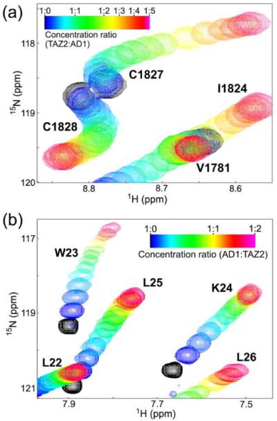
Portions of the ¹H–¹⁵N HSQC spectra of (a) TAZ2 showing chemical shift changes upon titration with p53 AD1(13–37) and (b) p53 AD1 showing chemical shift changes upon titration of TAZ2. The cross-peak color changes gradually from black (free) to magenta (bound) according to the concentration ratio.

Figure 2.

The SVD analysis of the ¹⁵N-TAZ2 titration with unlabeled p53 AD1. (a) Blue bars show the singular values sorted in decreasing order plotted in the logarithmic scale. Red circles show the RMSD (ppm) between the raw data set and the data set reconstructed using the 1 ~ i-th components (abscissa). Inclusion of all (1 ~ 17-th) components for the data reconstruction results in the RMSD of 0, which is not shown in the figure. Inset shows the autocorrelation of v_i vectors plotted against the component number. (b) The shape of v_i vectors for the first five components plotted against the number of titrations. First three components have smooth shape (thick lines with filled circles), resulting in high autocorrelation.

Local vs. global analysis

Accordingly, we analyzed the HSQC titration curves (Figure S2) assuming a two-site binding model (Scheme 1), where F is the free form of TAZ2, B1 and B2 are the singly bound forms in which only the primary (high affinity) site or the secondary (low affinity) site is occupied by p53, respectively, B12 is the doubly bound form, and L is the free form of the p53 subdomain (see Materials and Methods for details). K_d1, k_on1, and k_off1 are the equilibrium dissociation constant, the association rate, and the dissociation rate for primary binding, respectively, and K_d2, k_on2, and k_off2 are those for secondary binding. Correction for protein concentration was implemented in the fitting, because accurate determination of protein concentration is crucial for obtaining reliable fits. Fitting each titration curve independently (i.e., local fitting) did not give reliable K_d values; only the curves with large chemical shift changes gave reasonable fits but with large scatter (Figure S3a,b and Table 1). When we used the noise-filtered data set that was reconstructed using only the three non-noise components, many curves fitted better to the two-site binding model, especially when a concentration correction was implemented (Figure S3c,d and Table 1). However, the K_d values were still scattered, and had large standard deviations.

Scheme 1.

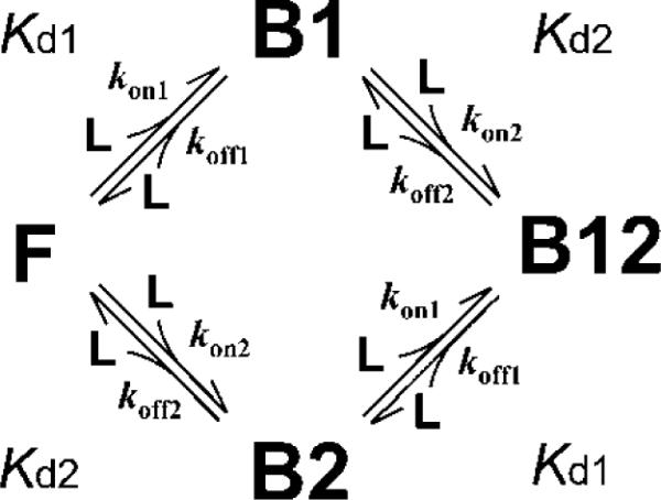
A two-site binding model.

Table 1.

Dissociation constants K_d1 and K_d2 for primary and secondary binding of unlabeled p53 AD1 with ¹⁵N-labeled TAZ2.

Method	Data seta	Correctionb	Number of curvesc	Kd1 (μM)	Kd2 (μM)
Local fit	raw	–	41	27 ± 27d	448 ± 788
Local fit	raw	1.0 ± 0.3	30	24 ± 26	345 ± 638
Local fit	SVD	–	57	33 ±14	225 ± 280
Local fit	SVD	1.1 ± 0.1	67	27 ± 14	126 ± 52
Global fite	raw	–	148	31 ± 2	180 ± 7
Global fit	raw	1.029 ± 0.009	148	27 ± 3	177 ± 6
Global fit	SVD	–	148	32 ± 2	169 ± 4
Global fit	SVD	1.071 ± 0.005	148	24 ± 1	164 ± 3

^aThe data set used for fitting: the raw data set (raw) or the reconstructed data set after noise filtering (SVD).

^bWith or without (−) correction for the TAZ2 concentration. The correction factor, cp, is described when the correction was implemented in the fitting.

^cFor local fits, only the good fits in which both K_d1 and K_d2 are within 10⁻⁶ ~ 10⁻² M and in which the fitting errors are smaller than the fitted values were used in calculating the average and standard deviation of the K_d values and the correction factor. The number of curves satisfying this criteria is shown. For global fits, all curves showing clear fast-exchange shifts were used for fitting.

^dStandard deviation.

^eFor global fit, errors were estimated by the Monte Carlo error estimation method.

On the other hand, fitting all titration curves globally (i.e., global fitting) gave reliable estimates of K_d1 and K_d2 with smaller errors (Table 1). Here, dissociation constants and a concentration correction factor are common for all curves, but the chemical shift differences between the free and the bound forms differ for each curve. All ¹H and ¹⁵N titration curves were fitted well to the common K_d values (Figure S2). Thus, global fitting is effective in accurately estimating dissociation constants. The use of the noise-filtered data set in the global fit with concentration correction further improved the model fitting and gave K_d1 and K_d2 of 24 and 164 μM, respectively, with smaller errors (Figures 3a and S4, and Table 1). Taken together, the global fit of titration curves after noise filtering is the most effective way of estimating accurate dissociation constants from HSQC titration experiments.

Figure 3.

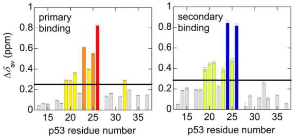
Global fitting of the noise-filtered titration curves for the ¹⁵N-TAZ2 titration with unlabeled p53 AD1. (a) Selection of the data from the global fit of chemical shift changes of HSQC cross peaks of ¹⁵N-TAZ2 as a function of the concentration ratio of AD1/TAZ2. Color codes are shown in the panel along with the residue number. (b) The histograms of the averaged chemical shift differences Δδ_av for the primary (upper) and secondary binding (lower). The black horizontal line shows the mean of all Δδ_av (0.081 and 0.104 ppm for primary and secondary binding, respectively). The residues are categorized into the following groups: (red or blue) mean + 2×SD ≤; (orange or cyan) mean + 1×SD ~ mean + 2×SD; (yellow or pale green) mean ~ mean + 1×SD; and (gray) < mean. (c) Mapping the location of the residues having large Δδ_av onto the NMR structure for the primary (upper) and secondary binding (lower). The color codes are the same as in (b). Three zinc binding sites and four α-helices are shown. Helix α1 corresponds to residues 1765–1785, α2 to 1794–1806, α3 to 1818–1833, and α4 to 1842–1852.

In addition to the dissociation constants, the global fit also gives the ¹H and ¹⁵N chemical shift differences between the free and the bound form for both primary and secondary binding (Figure S5). Effects of binding events on each residue are represented by an average chemical shift difference, $\Delta {\delta }_{\mathrm{av}}=\sqrt{{\left(\Delta {\delta }_{\mathrm{H}}\right)}^2+{(\Delta {\delta }_{\mathrm{N}}∕5)}^2}$ (Figure 3b).¹⁷ For the primary binding, a large chemical shift difference was observed especially for Val1802, Leu1823, and Leu1826 (Δδ_av greater than 2 × standard deviation (SD) from the mean). On the other hand, the secondary binding largely affected Ala1825, Cys1827, Tyr1829, and Lys1832. Mapping these residues onto the NMR structure of TAZ2 shows that the residues affected by the primary and secondary AD1 binding are located at two opposite faces of TAZ2 (Figure 3c).

Complementary titration

As an alternative way of measuring the same binding events, we measured the HSQC titrations of ¹⁵N-labeled AD1 with unlabeled TAZ2 (Figures 1b and S1b). The AD1 peaks also show fast- exchange shifts and a slight curvature, again indicating the presence of at least two binding modes. The SVD analysis indicates the presence of three non-noise components, one of which is the spectrum for the free form of AD1 (Figure S6a,b). Thus, the data set reconstructed using only the three non-noise components was globally fitted with the 2-site binding model to obtain K_d1 and K_d2 of 38 and 263 μM, respectively (Figure S6c and Table S1).

Although the K_d values are consistent with those obtained from the ¹⁵N-TAZ2 titration with AD1, they have larger uncertainties. This is because the secondary binding event is less prominent for the ¹⁵N-AD1 titration with TAZ2 compared with the ¹⁵N-TAZ2 titration with AD1 (Figure S7). Thus, it is preferable to titrate ligand (that binds at multiple sites) into ¹⁵N-labeled protein (that has multiple binding sites), in order to estimate accurate K_ds for multisite binding.

To estimate chemical shift changes for ¹⁵N-AD1, the titration curves were fitted using the K_ds obtained by ¹⁵N-TAZ2 titration with AD1 (Table 1). Upon binding of p53 AD1 to TAZ2, chemical shifts of residues 19 ~ 26 of p53 are affected (Figure 4), suggesting that this region interacts with TAZ2.

Figure 4.

The Δδ_av histograms of the primary (left) and secondary binding (right) obtained from the ¹⁵N-p53 AD1 titration with unlabeled TAZ2 using the K_ds obtained by the ¹⁵N-TAZ2 titration with AD1. The TAZ2 concentration correction factor was 1.08 ± 0.01. The black horizontal line shows the mean of all Δδ_av (0.251 and 0.286 ppm for primary and secondary binding, respectively). The residues are categorized into the groups as described in Figure 3b.

TAZ2:AD2 interactions

Next we performed the HSQC titration of ¹⁵N-labeled TAZ2 with the unlabeled AD2 peptide from p53 (Figure S8). The SVD analysis indicates the presence of three non-noise components, one of which is the spectrum for the free form of AD2 (Figure S9a,b; see Supporting Information for details). Thus, the data set reconstructed using only the three non-noise components was globally fitted to the 2-site binding model to get K_d1 and K_d2 of 32 nM and 10.2 μM, respectively (Table S2, Figures 5a and S10). The K_d1 value is close to the K_d for the binding of p53(13–61) to TAZ2 measured by fluorescence titrations (~10–20 nM), supporting the validity of this small value.¹⁸ A large chemical shift difference was observed especially at Val1819, Ala1825, and Leu1826 for the primary binding and at Thr1806, Cys1827, Lys1832, and Lys1838 for the secondary binding (Figure S9c). Although the HSQC cross peaks for Val1802 and Leu1823 broadened out at higher ratios and were not used for the global fit, their Δδ_av values at a 1:0.6 ratio were the seventh largest and the largest among all residues, respectively, indicating that both Val1802 and Leu1823 are greatly affected by the primary AD2 binding. The cross peak for Tyr1829 broadened out at higher than 1:2.5 ratios, but the chemical shift change between 1:1.0 and 1:2.5 ratios was the largest for Tyr1829 among all residues, indicating that Tyr1829 is strongly affected by the secondary binding. Mapping these residues onto the NMR structure of TAZ2 shows that the regions affected by the primary and secondary AD2 binding are very similar to those for the AD1 binding (Figure 5b).

Figure 5.

Global fitting of the noise-filtered titration curves for the ¹⁵N-TAZ2 titration with unlabeled p53 AD2. (a) Selection of the data from the global fit of chemical shift changes of HSQC cross peaks of ¹⁵N-TAZ2 as a function of the ratio of AD2/TAZ2. Color codes are shown in the panel along with the residue number. (b) Mapping the location of the residues having large Δδ_av onto the NMR structure for the primary (upper) and secondary binding (lower). The color codes are the same as in Figure 3b, except that Val1802 and Leu1823 are shown by magenta (upper) and Tyr1829 is shown by purple (lower).

Ranges of accurate K_d1 and K_d2 determined by NMR titrations

To accurately determine dissociation constants for one-site binding processes from titration experiments, the protein concentration should be close to K_d.² Given the relatively high protein concentration typically used for NMR detection (ca. 100 μM or greater), it is difficult to determine K_d in the nM range for single-site binding by NMR titrations, although the use of lower protein concentrations may expand the lower limit of K_d in favorable cases (see Supporting Information for details). In marked contrast, it is possible to accurately estimate a K_d1 of less than 100 nM by NMR titrations for two-site binding, even at high protein concentrations, because secondary binding reduces the occupancy of the primary site.¹² However, accurate estimates of both K_d1 and K_d2 require that the primary and secondary binding events are coupled; if the secondary binding event is very weak, then the situation once again approximates to a one-site binding event. Our previous simulations show that K_d1 of 10 nM ~ 1 μM can be reliably obtained by global fit if K_d2 is between 10¹ ~ 10³-fold of K_d1 and that, if the dissociation rate is rapid enough such that resonances shift in fast exchange, even a K_d1 of 1 nM can be measured if K_d2 is in the range 0.1 ~ 10 μM.¹²

To examine whether this conclusion holds when experimental conditions are changed such as the number of data points, a maximum titrant/protein ratio, protein concentration, and the number of peaks used in the analysis, we simulated titration curves by changing these conditions and examined whether the K_d1 and K_d2 values used for simulation can be reproduced by global fitting (Figure 6). Here, K_d1 and K_d2 were set as multiples of ten between 10⁻¹⁰ ~ 10⁻¹ M (K_d1 < K_d2), and chemical shift changes obtained for ¹⁵N-TAZ2 titration with AD1 (Figure S5) were used for simulations (see Materials and Methods for details). First, we changed the number of data points with fixing the maximum titrant/protein ratio to 1:5. For example, the number of data points was 25 when an interval of titrations was 1:0.2. The fitting simulations showed that the K_d1 of 10⁻⁹ ~ 10⁻⁴ M was accurately reproduced by global fitting, if K_d2 was 10¹ ~ 10³-fold of K_d1 (Figures 6a and S11). On the other hand, when an interval of titrations was 1:1 and the number of data points was 5, only the K_d1 of 10⁻⁷ ~ 10⁻⁴ M was reproduced by global fitting (Figure S11). Thus, the increase in the number of data points, i.e., the decrease in an interval of titrations, improves fitting and widens the ranges of sets of K_d1 and K_d2 that are accurately reproduced by global fitting. Therefore, it is preferable to measure titration curves at an interval of 1:0.2 (Figure 6a). Interestingly, the titration curves with an interval of 1:0.5 also gave good estimates of K_d1 and K_d2 (figure s11), probably because measurement at a 1:1 ratio is important for accurate estimates. In our experiments, we measured HSQC spectra at 1:0, 0.1, 0.2, 0.4, 0.6, 0.8, 1.0, 1.25, 1.5, 1.75, 2.0, 2.5, 3.0, 3.5, 4.0, 4.5, and 5.0 concentration ratios (17 data points), which are combinations of 1:0.2, 0.25, and 0.5 ratios. Thus, the present simulations show the validity of the use of these ratios for accurate estimates of K_d values. This set of concentration ratios was used in the following simulations.

Figure 6.

Dependence of accurate K_d1 and K_d2 ranges on (a) the number of data points (an interval of ratios), (b) a maximum titrant/protein ratio, (c) protein concentration, and (d) the number of peaks used in the analysis. Representative results are shown (see Figures S11–S14 for details). Conditions of fitting simulations are described in each panel. The red, orange, and yellow squares and cross symbols show that both the fitting errors and the differences between the fitted K_d and the input K_d used for generating the curves are less than 5%, 5 ~ 10%, 10 ~ 20%, and more than 20% of the input K_d values, respectively. Gray circles and diamonds show that only K_d1 or K_d2 were accurately obtained by global fit, because the binding events approached one-site binding at higher K_d2 or at lower K_d1, respectively. It should be noted that a K_d1 of less than 1 nM cannot be estimated by NMR titrations, because such a tight binding does not show fast-exchange shifts (see Figure 7).

Changing the maximum titrant/protein ratio in global fitting indicated that titration curves should be measured up to at least 1:2 ratio and, preferably, more than 1:3 ratio (Figures 6b and S12). Protein concentration dependence on titration experiments shows that lower K_ds are accurately estimated at lower protein concentrations and vice versa (Figures 6a,c and S13). Finally, changing the number of peaks used in global fitting indicated that the K_ds are more accurately estimated by using more resonance peaks (Figures 6d and S14); the use of a single peak (two curves from ¹H and ¹⁵N chemical shifts) does not give an accurate K_d1 in nM ranges, and the use of more than 20 peaks (40 curves) are preferable. Taken together, it is possible to accurately estimate a K_d1 in nM ranges, if the primary and secondary bindings are coupled and if the above criteria are satisfied. Our titration experiments fulfilled all these criteria, demonstrating the accuracy of the K_d values for the TAZ2:AD1/2 interactions.

Lower limit of accurate K_d1

An essential prerequisite for this analysis is that the chemical exchange process is in the fast-exchange regime. To estimate the K_d1 range showing fast exchange, we simulated a series of one-dimensional ¹H lineshapes for two-site binding at 1:0 ~ 1:5 concentration ratios, taking into account k_on and k_off rates explicitly. ¹H chemical shift changes for primary and secondary binding were assumed to be ~0.1 ppm, because the mean Δδ_H values for the primary and secondary binding of p53 AD1/2 with TAZ2 were 0.05 and 0.07 ppm, respectively. k_on and k_off were set as multiples of ten between 10⁴ ~ 10¹¹ M⁻¹s⁻¹ and between 10⁻² ~ 10⁸ s⁻¹, respectively. Combinations of k_on1, k_on2, k_off1, and k_off2 that satisfy K_d1 and K_d2 of 10⁻¹⁰ ~ 10⁻¹ M (K_d1 < K_d2) were used to calculate lineshapes (see Materials and Methods for details). For example, 336 combinations of rate constants satisfied a K_d1 of 1 μM, and 132 combinations among them showed fast exchange throughout titrations from 1:0 to 1:5 ratios; in other words, the fraction of fast exchange was 39% (= 132/336) at a K_d1 of 1 μM (Figures 7a and S15a). The simulations showed that the fraction of fast exchange is 0% at a K_d1 of 0.1 nM, increases with increasing K_d1, and finally reaches 100% at a K_d1 of more than 10⁻² M (Figure 7a). The results indicate that a K_d1 of 0.1 nM cannot be determined by NMR titrations, and the lower limit of K_d1 determined by the present method is 1 nM. Note that the lower limit of K_d1 also depends on chemical shift changes for the primary and secondary binding. When the ¹H chemical shift differences were assumed to be ~0.4 ppm in the lineshape simulations, close to the maximum Δδ_H for ¹⁵N-TAZ2 titrations with AD1 (Figure S5a), the lower limit of K_d1 became 10 nM (Figure S15b). Therefore, the lower limit of K_d1 that can be accurately determined by NMR titration ranges from 1 nM to 10 nM, depending on the particular system.

Figure 7.

(a) K_d1 dependence of the fraction of fast exchange for Scheme 1. Chemical shift changes were assumed to be ~0.1 ppm. Combinations of k_on1, k_on2, k_off1, and k_off2 that satisfy K_d1 and K_d2 of 10⁻¹⁰ ~ 10⁻¹ M (K_d1 < K_d2) were used to calculate lineshapes. Black open squares show the counts of the combinations of rate constants that produce the indicated K_d1 value. Red filled circles show the counts of the combinations of rate constants that show fast-exchange shifts throughout the titrations from 1:0 ~ 1:5 ratios. Green bars are the ratio of these values, corresponding to the fraction of fast exchange at the indicated K_d1 value. (b) The same as (a), except that the interconversion between B1 and B2 is taken into account (Scheme 2). (c) Increase in the fraction of fast exchange by the presence of the B1–B2 interconversion. The gray bar shows the ratio of the fraction of fast exchange in the presence of the B1–B2 interconversion (Scheme 2) to that in the absence of the interconversion (Scheme 1).

In Scheme 1, we neglected an interconversion between the B1 and B2 forms. However, it might be possible that the p53 AD1 or AD2 subdomain bound to one site of TAZ2 moves to another site without dissociation by Scheme 2, where k₁₂ and k₂₁ are the rate constants for the interconversion from B1 to B2 and from B2 to B1, respectively. The presence of the interconversion may affect the chemical shift time scale. As expected, lineshape simulations based on Scheme 2 showed that the presence of interconversion increases the fraction of fast exchange (Figure 7b); more than 40% increase in the fraction of fast exchange was observed at a K_d1 of 10⁻⁸ ~ 10⁻⁶ M (Figure 7c). Thus, fast exchange for a nM dissociation constant is not unrealistic, and our NMR titration analysis is also applicable to the cases of tight binding phenomena accompanied with rapid association/dissociation equilibrium.

Scheme 2.

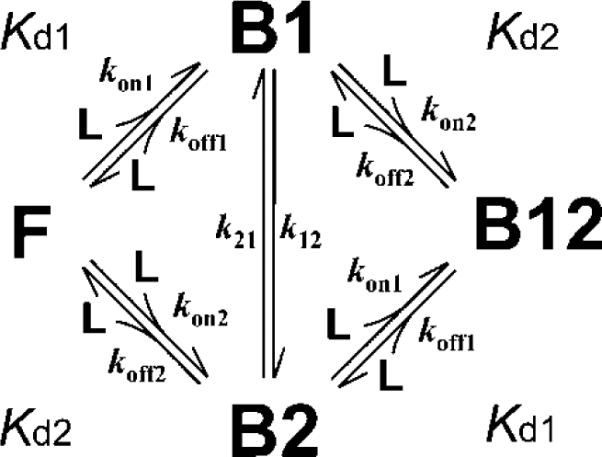
A two-site binding model with an interconversion between B1 and B2.

k_on and k_off rates for TAZ2:AD2 interactions

To estimate k_on and k_off that fulfill a small K_d1 of 32 nM for the TAZ2 interactions with AD2, we performed fitting of lineshapes of a series of titrations (see Materials and Methods for details). Here, one-dimensional slices of cross peaks in the ¹H dimension were used (Figures 8 and S16), and K_d1 and K_d2 were fixed to 32 nM and 10.2 μM, re-spectively. Global fitting of ¹H lineshapes for many peaks gave a k_on1 of (1.7 ± 0.2) × 10¹⁰ M⁻¹ s⁻¹, which is extremely fast but not beyond the diffusion-controlled limit (see below). k_off1 was estimated to be 540 ± 80 s⁻¹, which is reasonably fast to show fast-exchange shifts. On the other hand, k_on2 and k_off2 for the secondary TAZ2:AD2 binding were (7.1 ± 0.8) × 10⁸ M⁻¹ s⁻¹ and 7200 ± 900 s⁻¹, re-spectively. Thus, slower k_on and faster k_off compared with the primary binding resulted in larger K_d2.

Figure 8.

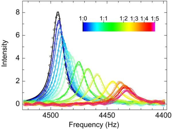
A series of ¹H lineshapes for Val1841 observed in the ¹H–¹⁵N HSQC titration of ¹⁵N-TAZ2 with unlabeled p53 AD2 in which TAZ2:AD2 concentration ratios ranged from 1:0 to 1:5. The lineshape color changes from black (free) to magenta (bound) according to the concentration ratio. Continuous lines are obtained from global fitting of lineshapes.

It should be noted that the fast k_on1 obtained by line-shape analysis is not an artifact due to assumptions introduced in the fitting, because a k_on1 of 10¹⁰ M⁻¹ s⁻¹ is readily predicted as follows. Fast-exchange shifts for TAZ2:p53 AD2 interaction imply that k_off1 ≥ 500 s⁻¹.¹ Here, K_d1 is 32 nM, suggesting that k_on1 = k_off1/K_d1 ≈ 500 / (32 × 10⁻⁹) ≈ 1.6 × 10¹⁰ M⁻¹ s⁻¹. Our lineshape analysis is fully consistent with this estimate.

Discussion

p53 AD1 and AD2 binding sites on TAZ2

Primary binding of the p53 AD1 peptide largely affects the chemical shifts of the residues located on a hydrophobic surface at the interface between the α1, α2, and α3 helices. This region corresponds to the binding site previously identified by chemical shift mapping using the p53(14–28) peptide.¹⁹ On the other hand, secondary binding of AD1 affects residues located on the opposite surface of TAZ2, composed mainly of residues in the α1, α3, and α4 helices. Because these two regions overlap with the binding sites of the STAT1-TAD²⁰ and E1A,²¹ it is reasonable to consider that the large chemical shift changes are due to direct interactions with AD1. The chemical shifts of some residues that are distant from the binding surfaces, such as Thr1806 and Lys1838, are also slightly affected by the secondary binding process, probably due to propagation of perturbations from the binding surfaces or local conformational changes rather than direct binding (see Supporting Information for more discussion). Recently Feng et al. have determined the NMR structure of the complex between TAZ2 from p300 and the p53(2–39) peptide.²² The structure is consistent with our chemical shift mapping results in that Val1802, Leu1823, and Leu1826 of TAZ2 have direct hydrophobic contacts with p53 and that residues 17 ~ 24 of the p53 AD1 subdomain form an α-helix upon binding.

Comparison between the primary and secondary binding sites indicates that the primary site is more hydrophobic than the secondary site. This suggests that hydrophobic interactions are important in stabilizing the TAZ2-p53 AD1 interactions.

Unexpectedly, the primary and secondary AD2 binding sites on TAZ2 overlap with those for AD1 binding. However, there is a slight difference between AD1 and AD2 binding. The primary binding site of AD2 overlaps with that of AD1 at Val1802, Leu1823, and Leu1826, but Val1819 and Ala1825 are also affected by AD2, indicating binding to a broader TAZ2 surface. The reason why AD2 binds more tightly than AD1 may be that highly negatively charged AD2 (−8.0) compared with AD1 (−2.0) is more favorable for the electrostatic interactions with the highly positively charged TAZ2 (+14.3).

Thus, AD1 and AD2 can bind to the same primary and secondary binding sites. However, in the full-length p53 TAD, AD1 and AD2 are connected by a linker, and it is unlikely that both of them can bind simultaneously to the primary site of a single TAZ2 molecule, considering the size of the binding site. Since the affinity of AD2 for the primary site is significantly higher than that of AD1 (K_d1 32 nM versus 24 μM), it is most likely that AD2 occupies the primary binding site and the AD1 the secondary site in the binary complex between TAZ2 and the full-length p53 TAD. In support of this, the titration of the AD2 peptide into the ¹⁵N-AD1:TAZ2 (1:1) complex competes out the ¹⁵N-AD1, but the titration of the AD1 peptide into the ¹⁵N-AD2:TAZ2 (1:1) complex only inefficiently competes out the ¹⁵N-AD2, indicating that both AD1 and AD2 bind the same high-affinity site on TAZ2 and that AD2 binds more tightly than AD1.

Extremely fast association rate for TAZ2:p53 binding

Previous studies have reported that a protein-protein association rate can be larger than 10⁹ M⁻¹ s⁻¹ (Table 2)^23–27; the hydroxylated HIF-1α/TAZ1 association rate was shown to be ~10⁹ M⁻¹ s⁻¹.²⁸ However, a k_on larger than 10¹⁰ M⁻¹ s⁻¹ has not yet been reported. To our knowledge, a k_on of 1.7 × 10¹⁰ M⁻¹ s⁻¹ for TAZ2 binding with p53 AD2 is the fastest association rate for protein-protein interactions.

Table 2.

Fast association rates for protein-protein, protein-ligand, and protein-nucleic acid interactions.

protein	target	Kon (M−1 s−1)	reference
Protein-protein
TAZ2	P53 AD2	1.7 × 1010	this study
barnase	barstar	> 5 × 109	26
E9 DNase	Im9	6 × 109	24
colicin E9	Im9	4 × 109	24
cytochrome peroxidase	cytochrome c	> 3 × 109	25
TAZ1	HIF-OH	1.3 × 109	28
Acetylcholin-esterase	fasciculin	1 × 109	27
Thrombin	hirudin	~1 × 109	23
Protein-ligand
Acetylcholin-esterase	TFK+	2~9 × 1010	27
Fumarase	famarate	3 × 1010	30
superoxide dismutase	superoxide	2 × 1010	31
Protein-nucleic acid
lac repressor	operator DNA	2 × 1010	44
Restrict	ribosomal RNA	1.7 × 1010	46
RNase A	RNA substrate	3 × 109	45

Although a diffusion-limited association rate was theoretically estimated to be 10⁹ ~ 10¹⁰ M⁻¹ s⁻¹ for two uniformly reactive spheres with an equal size,²⁹ the association rate for binding of the p53 AD2 subdomain to TAZ2 is not exceptionally large, if the size, geometry, and charges of the two interacting molecules are taken into account. First, an association rate can be faster if one molecule is small and diffuses rapidly while the other is large and provides a large target.²⁹ Indeed, fast association processes with a k_on of > 10¹⁰ M⁻¹ s⁻¹ have been reported for the interactions between a protein and a small ligand (Table 2).^27,30,31 Second, for a molecule with rodlike geometry (prolate ellipsoid), which can be adopted by nucleic acids, the effective capture radius approaches the length of the major semi-axis of the ellipsoid, leading to a higher association rate than a spherical molecule.²⁹ Although intrinsically disordered proteins (IDPs) often have more compact structures than chemically denatured proteins, they are more expanded than molten globules.^32–34 In accord with this, Wolynes and coworkers have predicted on theoretical grounds that the association rates of IDPs will be enhanced substantially by the “fly-casting” mechanism.^35,36 However, a recent study has suggested that a greater capture radius of an IDP also leads to slower translational diffusion, which opposes fast association.³⁷ Finally, particularly favorable, complementary electrostatic interactions can accelerate binding reactions dramatically, giving a k_on range of 10⁹ to 10¹¹ M⁻¹ s⁻¹.^26,38143 Consistent with this, association processes with a k_on of ~10¹⁰ M⁻¹ s⁻¹ have been reported for protein-nucleic acid interactions (Table 2).^44–46

The p53 AD2 motif fulfills these requirements: it is small, intrinsically unstructured in its free form, and has negative charges that favor electrostatic interaction with the highly positively charged TAZ2. Thus, a k_on of 1.7 × 10¹⁰ M⁻¹ s⁻¹ is within the range expected for binding processes of IDPs with favorable electrostatic interactions (see Supporting Information for more discussion). Among these requirements for fast association, complementary electrostatics probably plays a major role in determining the very rapid binding kinetics of the AD2 motif. Accordingly, k_on for the secondary AD2 binding process is slower, because the second p53 AD2 molecule experiences a smaller electrostatic driving force for binding after the reduction of the net positive charge on TAZ2 due to binding of the first AD2 molecule.

In general, IDPs tend to be deficient in hydrophobic residues necessary for folding and rich in charged residues, resulting in a large net charge at neutral pH.³⁴ Therefore, it is plausible that a large net charge causes both intrinsic disorder and rapid binding, suggesting that fast association is an intrinsic nature of IDPs.

This fast association rate is comparable to the helix folding rate. A relaxation time constant for helix folding is typically 0.2 ~ 2 μs.⁴⁷ In our experimental conditions, the TAZ2 and p53 AD2 concentrations are in the order of 10⁻⁴ M. Here, the binding rate constant is 10⁶ s⁻¹ (= 10¹⁰ M⁻¹ s⁻¹ × 10⁻⁴ M), which corresponds to 1 μs. This value is comparable to the helix folding rate. The protein concentrations in vivo are much lower than in our NMR studies, indicating that the binding time constant is longer than 1 μs, within which helix formation can occur. Therefore, even if the mechanism of TAZ2 recognition by p53 AD2 is conformational selection,⁴⁸ helix formation of AD2 can precede the TAZ2 binding reaction.

Conclusions

We have presented here a quantitative method to analyze two-site protein interactions monitored by NMR chemical shift perturbation. Our method extends the lower limit of K_d determined by NMR to the 1 ~ 10 nM range, under favorable exchange conditions. The method is applicable not only for protein-protein interactions, but also for protein-ligand interactions and for conformational changes in a single protein molecule. Application of the method to the binding of IDPs revealed the presence of two p53 AD1 binding sites on TAZ2. Moreover, these sites overlapped with the site of binding of AD2 on the hydrophobic surface of TAZ2, but AD2 binds to TAZ2 more tightly than AD1. These results highlight the complexity of the interactions between IDPs and their targets. Thus, careful investigation of binding interactions is necessary for understanding the molecular mechanisms involving IDPs and `hub' proteins such as transcriptional coactivators. The binding of AD2 to TAZ2 is extremely fast, approaching the diffusion-controlled limit and suggesting that intrinsic disorder plus complementary electrostatics can significantly accelerate protein binding interactions.

Materials and Methods

Protein expression and purification

Unlabeled and ¹⁵N-labeled TAZ2 (residues 1764–1855) domain of mouse CBP and unlabeled and ¹⁵N-labeled p53 AD1 (13–37) and AD2 (38–61) subdomains were expressed and purified as described previously.¹²

NMR spectroscopy

NMR spectra were recorded using Bruker 500, 600, and 800 MHz spectrometers and analyzed using NMRPipe⁴⁹ and NMRView.⁵⁰ Published backbone assignments for TAZ2 and p53 were used.¹²¹H-¹⁵N HSQC titrations were performed to characterize binding of the TAZ2 domain to the p53 AD1 and AD2 subdomains. Conditions were 20mM Tris-HCl (pH 6.8), 50mM NaCl, 1mM DTT, and 10% D₂O at 35°C. For ¹⁵N-TAZ2 titration with p53 AD2, the initial concentration of ¹⁵N-TAZ2 was 200 μM, and aliquots of concentrated p53 AD2 were titrated into the NMR tube. For ¹⁵N-TAZ2 titration with p53 AD1 and for ¹⁵N-p53 AD1 titration with TAZ2, the concentrations of ¹⁵N-TAZ2 and ¹⁵N-p53 AD1 were 200 μM throughout the titrations.

SVD analysis

In the SVD analysis, the chemical shift data of each HSQC spectrum were represented as a one-dimensional column vector that contains δH and δN values, d = {δ_H1, …, δ_Hi, …, δ_Hm, δ_N1,…, δ_Ni, …,δ_Nm}, where m is the number of peaks (or residues) used in the analysis, and i (= 1 ~ m) is the peak number. Then, the HSQC spectra obtained by a series of n titrations were represented as a 2m × n data matrix D, in which the j-th column (D)_j is given by the chemical shift vector d for the j-th titration. The SVD algorithm expresses the data matrix in the following form:

$$\mathit{D}={\mathit{UWV}}^{\mathrm{T}}$$ (2)

where U = (u₁, …, u_n) is an 2m × n matrix of orthogonal columns, which form a complete set of n basis chemical shift vectors u_i; W is a diagonal n × n matrix of singular values sorted in decreasing order; and V = (v₁, …, v_n) is an n × n matrix whose elements measure the proportion of each u_i basis vector attributable to each of the singular values.⁶ Eq 2 indicates that the chemical shift vector at any concentration ratio can be expressed as a linear superposition of the orthogonal u_i bases. In the ideal case without noise, the rank of the matrix D corresponds to the number of mathematically independent states. However, for real data with noise, the number of non-noise components, n_c, must be estimated by taking into account (1) the singular values, (2) the shape and the autocorrelation of the v_i vectors, and (3) the RMSD of the SVD reconstruction.^6,8 The i-th singular value corresponds to the weight of the u_i basis vector in reconstituting the data matrix, and thus the large singular value indicates the significance of the corresponding base. Because each v_i vector is described as a linear combination of p_F and p_Bi, the shape of the v_i vector corresponding to a non-noise component should have a smooth shape, and consequently, a high autocorrelation. Autocorrelation and shape of each u_i basis vector were not used for this purpose, because a one-dimensional chemical shift vector, d, usually does not have a smooth shape and its autocorrelation is close to 0 (Figure S17).

For independent multisite protein-protein interactions, the number of non-noise components thus obtained corresponds to the number of the binding sites + 1 (for the free form) according to eq 1. To confirm that the spectrum for the free form is one of the non-noise components, we used a chemical shift difference referenced to the free form, Δδ = δ_obs □ δ_F, in constructing the one-dimensional chemical shift vector d and then the data matrix D. The SVD results showed that the number of non-noise components is reduced by 1, demonstrating that the spectrum for the free form is indeed one of the non-noise components.

After the number of non-noise components n_c is determined, it is possible to reconstruct the data set using only the non-noise components and discarding the noise components. The component reduction (noise filtering) is done by constructing the reduced U, W, and V matrices using only the non-noise components, resulting in 2m × n_c, n_c × n_c, and n × n_c matrices, respectively. Then, the back calculation of the data matrix D using eq 2 provides the noise-filtered data matrix, the use of which will increase the reliability of the subsequent model fitting.

Binding models

In the present study, interactions of the p53 AD1 and AD2 subdomains with the TAZ2 domain of CBP showed two-site binding, according to the SVD analysis. In the subsequent global analysis, we assumed an independent two-site binding model. In this model, the TAZ2 domain of CBP exists in the free form (F), the singly bound forms (B1 and B2) in which only the primary (high affinity) site or the secondary (low affinity) site is occupied, respectively, and the doubly bound form (B12). The p53 subdomain in the free form is denoted as L. For a two-site binding model with no interconversion between B1 and B2 (Scheme 1), the frac-tions of the F, B1, B2, and B12 forms, f_F, f_B1, f_B2, and f_B12, respectively, are described as

$$\begin{array}{cc}\hfill & f_{\mathrm{F}}=\frac{K_{d1}{K}_{d2}}{K_{d1}{K}_{d2}+\left(K_{d1}{K}_{d2}\right)\left[\mathrm{L}\right]+{\left[\mathrm{L}\right]}^2}\hfill \\ \hfill & f_{\mathrm{B}1}=\frac{K_{d2}\left[\mathrm{L}\right]}{K_{d1}{K}_{d2}+\left(K_{d1}{K}_{d2}\right)\left[\mathrm{L}\right]+{\left[\mathrm{L}\right]}^2}\hfill \\ \hfill & f_{\mathrm{B}2}=\frac{K_{d1}\left[\mathrm{L}\right]}{K_{d1}{K}_{d2}+\left(K_{d1}{K}_{d2}\right)\left[\mathrm{L}\right]+{\left[\mathrm{L}\right]}^2}\hfill \\ \hfill & f_{\mathrm{B}12}=\frac{{\left[\mathrm{L}\right]}^2}{K_{d1}{K}_{d2}+\left(K_{d1}{K}_{d2}\right)\left[\mathrm{L}\right]+{\left[\mathrm{L}\right]}^2}\hfill \end{array}$$ (3)

where K_d1 and K_d2 are the dissociation constants for the primary and secondary binding, respectively, and [L] is the concentration of the free form of AD1 or AD2, which is a solution of the following cubic equation:

$$\begin{array}{cc}\hfill & {\left[\mathrm{L}\right]}^3+a{\left[\mathrm{L}\right]}^2+b\left[\mathrm{L}\right]+c=0\hfill \\ \hfill & a=2{\left[\mathrm{P}\right]}_{\mathrm{tot}}-{\left[\mathrm{L}\right]}_{\mathrm{tot}}+K_{\mathrm{d}1}+K_{\mathrm{d}2}\hfill \\ \hfill & b=({\left[\mathrm{P}\right]}_{\mathrm{tot}}-{\left[\mathrm{L}\right]}_{\mathrm{tot}})(K_{\mathrm{d}1}+K_{\mathrm{d}2})+K_{\mathrm{d}1}+K_{\mathrm{d}2}\hfill \\ \hfill & c=-K_{\mathrm{d}1}+K_{\mathrm{d}2}{\left[\mathrm{L}\right]}_{\mathrm{tot}}\hfill \end{array}$$ (4)

where [P]_tot and [L]_tot are the total concentrations of TAZ2 and AD1 (AD2), respectively. The closed-form solution of eq 4 has been reported:⁵¹

$$\left[\mathrm{L}\right]=-\frac{a}{3}+\frac{2}{3}\sqrt{(a^2-3b)}\cos \frac{\theta }{3}$$ (5)

where

$$\theta =\arccos \frac{-2a^3+9ab-27c}{2\sqrt{{(a^2-3b)}^3}}$$

When TAZ2 is ¹⁵N-labeled, the observed ¹H and ¹⁵N chemical shift difference referenced to the free form, Δδ_obs, is described as

$$\begin{array}{cc}\hfill \Delta {\delta }_{\mathrm{obs}}& =\frac{\left[\mathrm{B}1\right]+\left[\mathrm{B}12\right]}{{\left[\mathrm{P}\right]}_{\mathrm{tot}}}\Delta {\delta }_{\mathrm{FB}1}+\frac{\left[\mathrm{B}2\right]+\left[B12\right]}{{\left[\mathrm{P}\right]}_{\mathrm{tot}}}\Delta {\delta }_{\mathrm{FB}2}\hfill \\ \hfill & =(f_{\mathrm{B}1}+f_{\mathrm{B}12})\Delta {\delta }_{\mathrm{FB}1}+(f_{\mathrm{B}2}+f_{\mathrm{B}12})\Delta {\delta }_{\mathrm{FB}2}\hfill \\ \hfill & =\frac{\left[\mathrm{L}\right]}{K_{\mathrm{d}1}+\left[\mathrm{L}\right]}\Delta {\delta }_{\mathrm{FB}1}+\frac{\left[\mathrm{L}\right]}{K_{\mathrm{d}2}+\left[\mathrm{L}\right]}\Delta {\delta }_{\mathrm{FB}2}\hfill \end{array}$$ (6)

where [B1], [B2], and [B12] are the concentrations of the B1, B2, and B12 forms, respectively, Δδ_FB1 and Δδ_FB2 are the ¹H or ¹⁵N chemical shift difference between the free form and the B1 or B2 form, respectively. On the other hand, when p53 AD1 is ¹⁵N-labeled, Δδ_obs is described as

$$\begin{array}{cc}\hfill \Delta {\delta }_{\mathrm{obs}}& =\frac{\left[\mathrm{B}1\right]+\left[\mathrm{B}12\right]}{{\left[\mathrm{L}\right]}_{\mathrm{tot}}}\Delta {\delta }_{\mathrm{FB}1}+\frac{\left[\mathrm{B}2\right]+\left[B12\right]}{{\left[\mathrm{L}\right]}_{\mathrm{tot}}}\Delta {\delta }_{\mathrm{FB}2}\hfill \\ \hfill & =\frac{{\left[\mathrm{P}\right]}_{\mathrm{tot}}}{{\left[\mathrm{L}\right]}_{\mathrm{tot}}}\{(f_{\mathrm{B}1}+f_{\mathrm{B}12})\Delta {\delta }_{\mathrm{FB}1}+(f_{\mathrm{B}2}+f_{\mathrm{B}12})\Delta {\delta }_{\mathrm{FB}2}\}\hfill \\ \hfill & =\frac{{\left[\mathrm{P}\right]}_{\mathrm{tot}}}{{\left[\mathrm{L}\right]}_{\mathrm{tot}}}\left\{\frac{\left[\mathrm{L}\right]}{K_{\mathrm{d}1}+\left[\mathrm{L}\right]}\Delta {\delta }_{\mathrm{FB}1}+\frac{\left[\mathrm{L}\right]}{K_{\mathrm{d}2}+\left[\mathrm{L}\right]}\Delta {\delta }_{\mathrm{FB}2}\right\}\hfill \end{array}$$ (7)

For a two-site binding model in which the singly bound states B1 and B2 interconvert (Scheme 2), eqs 3~7 and the following equation holds:

$$\frac{k_{\text{off}1}{k}_{\text{on}2}{k}_{21}}{k_{\text{on}1}{k}_{\text{off}2}{k}_{12}}=\frac{K_{\mathrm{d}1}{k}_{21}}{K_{\mathrm{d}2}{k}_{12}}=1$$ (8)

Note that k₁₂ and k₂₁ cannot be determined by fitting the titration curves because the fitting function is the same for both Scheme 1 and Scheme 2. However, the ratio of k₁₂ to k₂₁ can be obtained from K_d1 and K_d2 using eq 8.

Global analysis

The titration curves monitored using both ¹H and ¹⁵N chemical shifts referenced to those of the free form, Δδ_H and Δδ_N, respectively, were locally or globally fitted with the two-site binding model (Scheme 1). In performing global fits, the dissociation constants are common for all curves, but the chemical shift differences between the free and the bound forms, Δδ_FB1 and Δδ_FB2, differ for each curve. The fitting was done with an in-house fitting program nmrKd written in Fortran using algorithms taken from Numerical Recipes.⁵² Accurate determination of the protein concentrations is crucial for obtaining reliable fits. Because TAZ2 concentration could not be determined accurately by UV absorbance due to the presence of DTT, concentration corrections were implemented in the fitting program. Thus, [P]_tot was replaced by c_p[P]_tot in the above equations, where c_p is a correction factor for the TAZ2 concentration and is set as a variable during the fitting procedure. The con-centration correction led to improved fits. The global fit of 2m titration curves for m peaks includes 4m + 2 adjustable parameters (or 4m + 3 when concentration correction was performed).

Non-linear least squares fits with the Levenberg-Marquardt (LM) algorithm were used to minimize a global X²:

$$X^2=\sum _{i=1}^{2m}\sum _{j=1}^n{\left[\frac{y_{\text{obs}}(i,j)-y_{\text{fit}}(i,j)}{\sigma (i,j)}\right]}^2$$ (9)

where 2m is a total number of titration curves; n is a total number of titration points; y_obs(i,j) and y_fit(i,j) are observed and fitted chemical shift differences at i-th curve and j-th titration point, respectively; and σ(i,j) is a standard deviation of each data point, which works as a weight of the data point. Appropriate estimate of σ is necessary for global analysis, because only the curves with large Δδ_obs would be optimized if all data points had the same σ. When σ was not known, the σ for each titration curve was estimated by repeating the LM fit as follows: (1) an initial LM fit was performed assuming that all σ values are 1; (2) the RMSD was calculated for each titration curve; (3) the RMSD of the curve was used to determine σ for the data points involved in the curve and the data were then refitted using the LM method; (4) steps (2) and (3) were repeated until the σ values for all curves converged. This procedure gave a reasonable estimate of σ for all curves.

The Monte Carlo error estimation method was used to estimate the fitted parameters and the corresponding errors.⁵² Here, an initial global fit was performed using the actual data set. The RMSD between the actual and fitted curves was calculated for each curve. Then, ~100 hypothetical data sets were synthesized by using the initially fitted parameters and adding to each data point a random error calculated as (a random number with a normal distribution) × (RMSD of the corresponding curve). Each of the synthetic data sets was globally fit to obtain its fitted parameter set. The mean and standard deviation of these ~100 fitted parameter sets were used as the final fitted value and the corresponding error.

Peaks that are unassigned, noisy, or invisible because of intermediate exchange were not used in the combined SVD and global analysis. For ¹⁵N-TAZ2 titration with AD1, a total of 74 out of 92 residues of TAZ2 were used (148 curves and 17 titration points; a total of 2516 data points). For ¹⁵N-TAZ2 titration with AD2, a total of 68 residues of TAZ2 were used (136 curves and 16 titration points; 2176 data points). For ¹⁵N-AD1 titration with TAZ2, a total of 21 peaks of AD1 were used (42 curves and 13 titration points; 546 data points).

Fitting simulations

Fitting simulations were performed with various dissociation constants K_d1 and K_d2, by changing the number of data points (an interval of ratios), the maximum titrant/protein ratio, protein concentration, and the number of peaks used for analysis. The titration curves were generated using the Δδ_FB1 and Δδ_FB2 values obtained by titrating AD1 into ¹⁵N-labeled TAZ2 (Figure S5), assuming that the K_d1 and K_d2 values are a power of 10 between 10⁻¹⁰ and 10⁻¹ M (see the grid points in Figure 6; K_d1 < K_d2). A small amount of noise was added to each data point to simulate actual experimental data, as described above in the Monte Carlo error estimation method. Then, a global fit was performed for each K_d set, and the fitted K_d values were compared with those used in generating the titration curves. Fits were considered to be good if both the fitting errors and the differences between the fitted K_d and the input K_d used for generating the curves were within 10% of the input K_d values.

Lineshape simulations

The quantum mechanical density matrix formalism was used for the lineshape analysis.^53,54 Excited magnetization at each resonance frequency M(ν) is calculated by

$$M\left(v\right)=-\text{Re}\left({\mathbf{I}}^{-}{\mathbf{M}}_0^{-1}\sigma \right)$$ (10)

where I^□ is a row vector in which all elements are equal to 1. σ is a column vector represented by

$$\sigma =C\{f_{\mathrm{F}},f_{\mathrm{B}1},f_{\mathrm{B}2},f_{\mathrm{B}12}\}$$ (11)

where C is a constant, and f_F, f_B1, f_B2, and f_B12 are frac1 tions of F, B1, B2, and B12 forms, respectively, which are calculated from eq 3. For Scheme 2 with the interconversion between B1 and B2, the complex matrix M₀ is

$${\mathbf{M}}_0=\left(\begin{array}{cccc}\hfill a_1\hfill & \hfill k_{\text{off}1}\hfill & \hfill k_{\text{off}2}\hfill & \hfill 0\hfill \\ \hfill k_{\text{on}1}L\hfill & \hfill a_2\hfill & \hfill k_{21}\hfill & \hfill k_{\text{off}2}\hfill \\ \hfill k_{\text{on}2}L\hfill & \hfill k_{12}\hfill & \hfill a_3\hfill & \hfill k_{\text{off}1}\hfill \\ \hfill 0\hfill & \hfill k_{\text{on}2}L\hfill & \hfill k_{\text{on}1}L\hfill & \hfill a_4\hfill \end{array}\right)$$ (12)

$$\begin{array}{cc}\hfill & a_1=-k_{\text{on}1}L-k_{\text{on}2}L-R_{2\mathrm{F}}+2\pi i(v_{\mathrm{F}}-v)\hfill \\ \hfill & a_2=k_{\text{off}1}-k_{\text{on}2}L-k_{12}-R_{2\mathrm{B}1}+2\pi i(v_{\mathrm{B}1}-v)\hfill \\ \hfill & a_3=k_{\text{on}1}L-k_{\text{off}2}-k_{21}-R_{2\mathrm{B}2}+2\pi i(v_{\mathrm{B}2}-v)\hfill \\ \hfill & a_4=k_{\text{off}1}-k_{\text{off}2}-R_{2\mathrm{B}12}+2\pi i(v_{\mathrm{B}12}-v)\hfill \end{array}$$ (13)

where ν_i and R_2i (i = F, B1, B2, and B12) are the chemical shift and the transverse relaxation rate in the absence of chemical exchange, respectively. For Scheme 1 without the interconversion between B1 and B2, k₁₂ = k₂₁= 0. The R_2i values were assumed to be 20 s⁻¹ for all forms. ¹H chemical shift changes for primary and secondary binding were assumed to be ~0.1 ppm. Consequently, the ν_i values were assumed to be □50, □10, 10, and 50 Hz for the F, B1, B2, and B12 forms, respectively. Calculations were also performed assuming ¹H chemical shift changes of ~0.4 ppm (□200, □10, 10, and 200 Hz for the F, B1, B2, and B12 forms, respectively). Complex eigenvalues and eigenvectors of the matrix M₀ were calculated using LAPACK. k_on1, k_on2, k_off1, and k_off2 were set as multiples of ten between 10⁴ ~ 10¹¹ M⁻¹s⁻¹ and between 10⁻² ~ 10⁸ s⁻¹, respectively. k₁₂ and k₂₁ were assumed to be multiples of ten between 10⁻² ~ 10⁸ s⁻¹. Combinations of k_on1, k_on2, k_off1, k_off2, k₁₂, and k₂₁ that satisfy K_d1 and K_d2 of 10⁻¹⁰ ~ 10⁻¹ M (K_d1 < K_d2) were used to calculate lineshapes. Protein concentrations were the same as those used for the TAZ2 titration with AD1. A lineshape was considered to be that of fast exchange, if there is a single peak and its intensity is higher than one tenth of the peak intensity for the free form at a 1:0 ratio.

Lineshape fitting

To estimate k_on and k_off, the ¹H lineshapes of a series of p53 AD2 titrations into ¹⁵N-TAZ2 measured using the 500 MHz spectrometer were globally fitted with the two-site binding model (Scheme 1). All spectra were processed without apodization but with 8192 point zero-filling to increase the number of data points in the ¹H dimension. One-dimensional slices in the ¹H dimension were obtained at the top of cross peaks from the NMRView-format files, regions including other peaks were removed from the slices, and a set of ¹H lineshapes for a series of AD2 titrations into TAZ2 were obtained for each peak.

The fitting was done with an in-house fitting program glove_lineshape written in Fortran using algorithms taken from Numerical Recipes.⁵² As similar to nmrKd, the program uses the LM fitting algorithm, and can globally fit lineshapes of many peaks. Lineshapes were calculated using the quantum mechanical density matrix formalism as described above.^53,54 In performing global fits, k_on1, k_on2, k_off1, and k_off2 were common for all curves, but independent parameters were k_on1 and k_on2 only, because K_d1 and K_d2 were fixed to the values obtained from the titration curve analysis. Correction for TAZ2 concentration was implemented as similar to nmrKd, and a correction factor c_p was fixed to the value obtained from the analysis of titration curves. The frequencies in Hertz and the R₂ in s⁻¹ for the F, B1, B2, and B12 forms differ for each peak. The initial estimates of frequencies were obtained from titration curve analysis. Because the population of B2 is very low, lineshape fitting could not accurately estimate the frequency and R₂ for B2. Thus, the frequency of B2 was fixed to the value estimated from the titration curve analysis, and the R₂ of B2 was assumed to be the same as that of B1. In addition, an adjustable parameter for peak intensity was introduced for each lineshape, to account for changes in peak intensities accompanied with titrations. The initial estimates of R₂ values and peak intensities were obtained by fitting the lineshape of the free form. The global fit for m peaks and n titrations includes m (n + 7) + 3 adjustable parameters. Fitting errors were obtained from a covariance matrix.

Overlapping peaks were not used in the fitting. Moreover, lineshapes were not fit well when they had low intensities, distorted shapes, and small peak shifts. Consequently, only the following 12 peaks gave a reasonably good global fit: Val1781, His1782, Cys1791, Gln1797, Arg1801, Val1803, Thr1806, Lys1807, Cys1820, Val1841, Lys1848, and His1849. A total of 192 lineshapes and 18,009 data points were used for fitting (279 parameters). The fitted R₂ values for the F, B1 (B2), and B12 forms were, on average, 36, 41, and 49 s⁻¹, respectively.

ABBREVIATIONS

CBP

cyclic-AMP response element binding protein (CREB) binding protein

HSQC

heteronuclear single quantum correlation

IDP

intrinsically disordered protein

LM

Levenberg-Marquardt

RMSD

root mean square deviation

SD

standard deviation

SVD

singular value decomposition

TAD

transactivation domain

TAZ2

transcriptional adapter zinc finger 2

REFERENCES

- (1).Cavanagh J, Fairbrother WJ, Palmer AG, III, Rance M, Skelton NJ. Protein NMR Spectroscopy: Principles and Practice. Elsevier Academic Press; Burlington, MA: 2007. [Google Scholar]
- (2).Fielding L. Prog. NMR Spectros. 2007;51:219. [Google Scholar]
- (3).Henry ER, Hofrichter J. Methods Enzymol. 1992;210:129. [Google Scholar]
- (4).Jaumot J, Vives M, Gargallo R. Anal. Biochem. 2004;327:1. doi: 10.1016/j.ab.2003.12.028. [DOI] [PubMed] [Google Scholar]
- (5).Beechem JM. Methods Enzymol. 1992;210:37. doi: 10.1016/0076-6879(92)10004-w. [DOI] [PubMed] [Google Scholar]
- (6).Chen L, Hodgson KO, Doniach S. J. Mol. Biol. 1996;261:658. doi: 10.1006/jmbi.1996.0491. [DOI] [PubMed] [Google Scholar]
- (7).Ionescu RM, Smith VF, O'Neill JC, Jr., Matthews CR. Biochemistry. 2000;39:9540. doi: 10.1021/bi000511y. [DOI] [PubMed] [Google Scholar]
- (8).Arai M, Iwakura M. J. Mol. Biol. 2005;347:337. doi: 10.1016/j.jmb.2005.01.033. [DOI] [PubMed] [Google Scholar]
- (9).Jaumot J, Marchan V, Gargallo R, Grandas A, Tauler R. Anal. Chem. 2004;76:7094. doi: 10.1021/ac049509t. [DOI] [PubMed] [Google Scholar]
- (10).Matsuura H, Shimotakahara S, Sakuma C, Tashiro M, Shindo H, Mochizuki K, Yamagishi A, Kojima M, Takahashi K. Biol. Chem. 2004;385:1157. doi: 10.1515/BC.2004.149. [DOI] [PubMed] [Google Scholar]
- (11).Sakurai K, Goto Y. Proc. Natl. Acad. Sci. USA. 2007;104:15346. doi: 10.1073/pnas.0702112104. [DOI] [PMC free article] [PubMed] [Google Scholar]
- (12).Ferreon JC, Lee CW, Arai M, Martinez-Yamout MA, Dyson HJ, Wright PE. Proc. Natl. Acad. Sci. USA. 2009;106:6591. doi: 10.1073/pnas.0811023106. [DOI] [PMC free article] [PubMed] [Google Scholar]
- (13).Gu W, Shi XL, Roeder RG. Nature. 1997;387:819. doi: 10.1038/42972. [DOI] [PubMed] [Google Scholar]
- (14).Lill NL, Grossman SR, Ginsberg D, DeCaprio J, Livingston DM. Nature. 1997;387:823. doi: 10.1038/42981. [DOI] [PubMed] [Google Scholar]
- (15).Bochkareva E, Kaustov L, Ayed A, Yi GS, Lu Y, Pineda-Lucena A, Liao JC, Okorokov AL, Milner J, Arrowsmith CH, Bochkarev A. Proc. Natl. Acad. Sci. USA. 2005;102:15412. doi: 10.1073/pnas.0504614102. [DOI] [PMC free article] [PubMed] [Google Scholar]
- (16).Di Lello P, Jenkins LM, Jones TN, Nguyen BD, Hara T, Yamaguchi H, Dikeakos JD, Appella E, Legault P, Omichinski JG. Mol. Cell. 2006;22:731. doi: 10.1016/j.molcel.2006.05.007. [DOI] [PubMed] [Google Scholar]
- (17).Grzesiek S, Bax A, Clore GM, Gronenborn AM, Hu JS, Kaufman J, Palmer I, Stahl SJ, Wingfield PT. Nat. Struct. Biol. 1996;3:340. doi: 10.1038/nsb0496-340. [DOI] [PubMed] [Google Scholar]
- (18).Lee CW, Ferreon JC, Ferreon AC, Arai M, Wright PE. Proc. Natl. Acad. Sci. USA. 2010;107:19290. doi: 10.1073/pnas.1013078107. [DOI] [PMC free article] [PubMed] [Google Scholar]
- (19).De Guzman RN, Liu HY, Martinez-Yamout M, Dyson HJ, Wright PE. J. Mol. Biol. 2000;303:243. doi: 10.1006/jmbi.2000.4141. [DOI] [PubMed] [Google Scholar]
- (20).Wojciak JM, Martinez-Yamout MA, Dyson HJ, Wright PE. EMBO J. 2009;28:948. doi: 10.1038/emboj.2009.30. [DOI] [PMC free article] [PubMed] [Google Scholar]
- (21).Ferreon JC, Martinez-Yamout MA, Dyson HJ, Wright PE. Proc. Natl. Acad. Sci. USA. 2009;106:13260. doi: 10.1073/pnas.0906770106. [DOI] [PMC free article] [PubMed] [Google Scholar]
- (22).Feng H, Jenkins LM, Durell SR, Hayashi R, Mazur SJ, Cherry S, Tropea JE, Miller M, Wlodawer A, Appella E, Bai Y. Structure. 2009;17:202. doi: 10.1016/j.str.2008.12.009. [DOI] [PMC free article] [PubMed] [Google Scholar]
- (23).Stone SR, Dennis S, Hofsteenge J. Biochemistry. 1989;28:6857. doi: 10.1021/bi00443a012. [DOI] [PubMed] [Google Scholar]
- (24).Wallis R, Moore GR, James R, Kleanthous C. Biochemistry. 1995;34:13743. doi: 10.1021/bi00042a004. [DOI] [PubMed] [Google Scholar]
- (25).Mei H, Wang K, McKee S, Wang X, Waldner JL, Pielak GJ, Durham B, Millett F. Biochemistry. 1996;35:15800. doi: 10.1021/bi961487k. [DOI] [PubMed] [Google Scholar]
- (26).Schreiber G, Fersht AR. Nat. Struct. Biol. 1996;3:427. doi: 10.1038/nsb0596-427. [DOI] [PubMed] [Google Scholar]
- (27).Radic Z, Kirchhoff PD, Quinn DM, McCammon JA, Taylor P. J. Biol. Chem. 1997;272:23265. doi: 10.1074/jbc.272.37.23265. [DOI] [PubMed] [Google Scholar]
- (28).Sugase K, Lansing JC, Dyson HJ, Wright PE. J. Am. Chem. Soc. 2007;129:13406. doi: 10.1021/ja0762238. [DOI] [PMC free article] [PubMed] [Google Scholar]
- (29).Berg OG, von Hippel PH. Annu. Rev. Biophys. Biophys. Chem. 1985;14:131. doi: 10.1146/annurev.bb.14.060185.001023. [DOI] [PubMed] [Google Scholar]
- (30).Alberty RA, Hammes GG. J. Phys. Chem. 1958;62:154. [Google Scholar]
- (31).Sharp K, Fine R, Honig B. Science. 1987;236:1460. doi: 10.1126/science.3589666. [DOI] [PubMed] [Google Scholar]
- (32).Marsh JA, Forman-Kay JD. Biophys. J. 2010;98:2383. doi: 10.1016/j.bpj.2010.02.006. [DOI] [PMC free article] [PubMed] [Google Scholar]
- (33).Muller-Spath S, Soranno A, Hirschfeld V, Hofmann H, Ruegger S, Reymond L, Nettels D, Schuler B. Proc. Natl. Acad. Sci. USA. 2010;107:14609. doi: 10.1073/pnas.1001743107. [DOI] [PMC free article] [PubMed] [Google Scholar]
- (34).Uversky VN. Protein Sci. 2002;11:739. doi: 10.1110/ps.4210102. [DOI] [PMC free article] [PubMed] [Google Scholar]
- (35).Levy Y, Wolynes PG, Onuchic JN. Proc. Natl. Acad. Sci. USA. 2004;101:511. doi: 10.1073/pnas.2534828100. [DOI] [PMC free article] [PubMed] [Google Scholar]
- (36).Shoemaker BA, Portman JJ, Wolynes PG. Proc. Natl. Acad. Sci. USA. 2000;97:8868. doi: 10.1073/pnas.160259697. [DOI] [PMC free article] [PubMed] [Google Scholar]
- (37).Huang Y, Liu Z. J. Mol. Biol. 2009;393:1143. doi: 10.1016/j.jmb.2009.09.010. [DOI] [PubMed] [Google Scholar]
- (38).Eigen M, Hammes GG. Adv. Enzymol. 1963;25:1. doi: 10.1002/9780470122709.ch1. [DOI] [PubMed] [Google Scholar]
- (39).Fersht AR. Structure and mechanism in protein science: A guide to enzyme catalysis and protein folding. W. H. Freeman and Co.; New York, NY: 1999. [Google Scholar]
- (40).Sheinerman FB, Norel R, Honig B. Curr. Opin. Struct. Biol. 2000;10:153. doi: 10.1016/s0959-440x(00)00065-8. [DOI] [PubMed] [Google Scholar]
- (41).Schreiber G. Curr. Opin. Struct. Biol. 2002;12:41. doi: 10.1016/s0959-440x(02)00287-7. [DOI] [PubMed] [Google Scholar]
- (42).Levy Y, Onuchic JN, Wolynes PG. J. Am. Chem. Soc. 2007;129:738. doi: 10.1021/ja065531n. [DOI] [PubMed] [Google Scholar]
- (43).Schreiber G, Haran G, Zhou HX. Chem. Rev. 2009;109:839. doi: 10.1021/cr800373w. [DOI] [PMC free article] [PubMed] [Google Scholar]
- (44).Winter RB, Berg OG, von Hippel PH. Biochemistry. 1981;20:6961. doi: 10.1021/bi00527a030. [DOI] [PubMed] [Google Scholar]
- (45).Park C, Raines RTJ. Am. Chem. Soc. 2001;123:11472. doi: 10.1021/ja0164834. [DOI] [PubMed] [Google Scholar]
- (46).Korennykh AV, Piccirilli JA, Correll CC. Nat. Struct. Mol. Biol. 2006;13:436. doi: 10.1038/nsmb1082. [DOI] [PMC free article] [PubMed] [Google Scholar]
- (47).Mukherjee S, Chowdhury P, Bunagan MR, Gai FJ. Phys. Chem. B. 2008;112:9146. doi: 10.1021/jp801721p. [DOI] [PubMed] [Google Scholar]
- (48).Boehr DD, Nussinov R, Wright PE. Nat. Chem. Biol. 2009;5:789. doi: 10.1038/nchembio.232. [DOI] [PMC free article] [PubMed] [Google Scholar]
- (49).Delaglio F, Grzesiek S, Vuister GW, Zhu G, Pfeifer J, Bax AJ. Biomol. NMR. 1995;6:277. doi: 10.1007/BF00197809. [DOI] [PubMed] [Google Scholar]
- (50).Johnson BA, Blevins RA. J. Biomol. NMR. 1994;4:603. doi: 10.1007/BF00404272. [DOI] [PubMed] [Google Scholar]
- (51).Wang ZX, Jiang RF. FEBS Lett. 1996;392:245. doi: 10.1016/0014-5793(96)00818-6. [DOI] [PubMed] [Google Scholar]
- (52).Press WH, Flannery BP, Teukolsky SA, Vetterling WT. Numerical recipes in Fortran : The art of scientific computing. 2nd ed. Cambridge University Press; Cambridge, UK: 1992. [Google Scholar]
- (53).Binsch GJ. Am. Chem. Soc. 1969;91:1304. [Google Scholar]
- (54).Kern D, Kern G, Scherer G, Fischer G, Drakenberg T. Biochemistry. 1995;34:13594. doi: 10.1021/bi00041a039. [DOI] [PubMed] [Google Scholar]
Associated Data
This section collects any data citations, data availability statements, or supplementary materials included in this article.