The Number of Alleles at a Microsatellite Defines the Allele Frequency Spectrum and Facilitates Fast Accurate Estimation of θ

Abstract

Theoretical work focused on microsatellite variation has produced a number of important results, including the expected distribution of repeat sizes and the expected squared difference in repeat size between two randomly selected samples. However, closed-form expressions for the sampling distribution and frequency spectrum of microsatellite variation have not been identified. Here, we use coalescent simulations of the stepwise mutation model to develop gamma and exponential approximations of the microsatellite allele frequency spectrum, a distribution central to the description of microsatellite variation across the genome. For both approximations, the parameter of biological relevance is the number of alleles at a locus, which we express as a function of θ, the population-scaled mutation rate, based on simulated data. Discovered relationships between θ, the number of alleles, and the frequency spectrum support the development of three new estimators of microsatellite θ. The three estimators exhibit roughly similar mean squared errors (MSEs) and all are biased. However, across a broad range of sample sizes and θ values, the MSEs of these estimators are frequently lower than all other estimators tested. The new estimators are also reasonably robust to mutation that includes step sizes greater than one. Finally, our approximation to the microsatellite allele frequency spectrum provides a null distribution of microsatellite variation. In this context, a preliminary analysis of the effects of demographic change on the frequency spectrum is performed. We suggest that simulations of the microsatellite frequency spectrum under evolutionary scenarios of interest may guide investigators to the use of relevant and sometimes novel summary statistics.

Introduction

Microsatellite data are commonly employed in modern methods of population genetic inference. Their use in this context is recommended by several advantageous properties, including high mutation rates that facilitate inference on very recent events and relative ease of data acquisition in nonmodel organisms. In addition, some microsatellites may be targets of natural selection (e.g., Rockman and Wray 2002, Fondon and Garner 2004, Hammock and Young 2005, Vinces et al. 2009, Kozlowski et al. 2010). Both the microsatellite-based inference and the detection of functional microsatellites should benefit from an improved understanding of expected patterns of neutral microsatellite variation. For example, the equilibrium frequency spectrum of single nucleotide polymorphisms (SNPs) provides the null distribution for several influential tests for natural selection (Tajima 1989, Fu and Li 1993, Fay and Wu 2000). This suggests that the microsatellite frequency spectrum might prove similarly useful in a variety of inferential contexts. However, theoretical work has not produced a microsatellite analog to the SNP frequency spectrum.

The Microsatellite Allele Frequency Spectrum

To explore equilibrium expectations of microsatellite data, a mathematical model of microsatellite evolution is first required. Such a model enables forward and backward simulation of data as well as derivation of theoretical formulas. First proposed by Ohta and Kimura (1973) for allozyme variation, the stepwise mutation model (SMM) has since been co-opted as a common model of microsatellite evolution. The SMM posits that each mutation at a microsatellite locus is equally likely to increase or decrease repeat number by one step. Complications such as multistep mutation and biases in the direction of mutation are not incorporated in the SMM, though empirical evidence supports their occurrence (DiRienzo et al. 1994, rubinsztein95, Ellegren 2000, Xu et al. 2000).

Despite its relative simplicity, the SMM leads to patterns of variation that are more difficult to interpret than those of sequence data. Most importantly, recurrent mutation at a microsatellite locus generates homoplastic alleles that are identical by state but not identical by descent. This contrasts with sequence evolution under the infinite alleles (Kimura and Crow 1964) and infinite sites (Kimura 1969) models, where each SNP reflects the underlying genealogy with complete fidelity. Unlike microsatellites, closed-form solutions for the sampling distribution and allele frequency spectrum of SNPs quickly followed the introduction of the models that described their evolution (Ewens 1972, Watterson 1975).

Nevertheless, a number of important analytical results have been obtained for microsatellites. Moran (1975) showed that under the SMM the ordered distribution of allele frequencies at a locus, $\left\{p_i\right\}=\dots ,p_2,p_3,p_4,\dots$, does not have a limiting distribution. Mean allele type changes with time and $\left\{p_i\right\}$ moves up and down the i axis. However, if mean allele type is set to size zero and other types are adjusted accordingly, $\left\{p_i\right\}$ has a symmetric exponential form at equilibrium (Beder 1988, valdes93) and some of its moments have limiting distributions (Moran 1975). The moment $C_j=E[{\sum }_i{p}_i{p}_{i+j}]$, in particular, has been investigated in detail and specifies the probability that two randomly chosen alleles are separated by j steps (Ohta and Kimura 1973, Brown et al. 1975, Moran 1975). Numerous studies have explored the relationship between divergence time and genetic distance at a microsatellite locus, leading to the important result that this relationship is linear for certain genetic distances (Goldstein et al. 1995a,1995b; Zhivotovsky and Feldman 1995, Sun et al. 2009). Pritchard and Feldman (1996) investigated the divergence measure s, which is the difference in repeat number between two individuals, providing formulas for the expected value of s² and its variance under a variety of conditions including structured and bottlenecked populations.

Despite these and other theoretical advances, a closed-from solution for the microsatellite frequency spectrum remains unknown. In contrast to the relatively well-studied frequency distribution of allele types at a single locus (the previously described $\left\{p_i\right\}$), the microsatellite allele frequency spectrum (the frequency distribution of allele frequencies across the genome) has received little analytical attention. Kimura and Ohta (1975, 1978) provided a frequency spectrum for alleles evolving under the SMM, which they noted as possessing high frequencies of low-frequency alleles compared with the infinite sites model. However, their formula was derived under the assumption of small θ. This assumption is violated by the highly mutable microsatellites that are commonly analyzed. Recently, using both theory and empirical microsatellite data, Rosenberg and Jakobsson (2008) demonstrated the tight correspondence between the expected homozygosity and the frequency of the most frequent allele. This important relationship is a fundamental characteristic of the microsatellite frequency spectrum. Yet, a broadly applicable function for the allele frequency spectrum itself remains unavailable.

Estimating θ

Existing methods for estimating the scaled mutation parameter ($\theta =4N_{\text{e}}\mu$, where N_e is effective population size and μ is the per-locus mutation rate) exhibit variable performance. For example, two moment estimators of θ are easily calculated from summary statistics. The first is

(1)

where V_AS is variance in allele size (Moran 1975, Wehrhahn 1975). exhibits exorbitant variance (Xu and Fu 2004) but is unbiased and frequently employed in empirical studies. The second moment estimator is

(2)

where H is the unbiased estimate of homozygosity (Ohta and Kimura 1973, Kimmel et al. 1998). Though biased, exhibits considerably reduced error relative to (RoyChoudhury and Stephens 2007). In addition to moment estimators, several likelihood and Bayesian approaches to the estimation of microsatellite θ have been implemented (Nielsen 1997, Wilson and Balding 1998, stephens00, Beerli and Felsenstein 2001, RoyChoudhury and Stephens 2007). These methods use more of the data and require increased computation time.

Here, we report our approximate approach to deriving the microsatellite allele frequency spectrum and three new estimators of θ. We first develop a gamma approximation to the microsatellite allele frequency spectrum based on coalescent simulations. In the course of its development, we note the fundamental interrelationship of the frequency spectrum, θ, and n_a, the number of alleles sampled at a locus: 1) the microsatellite frequency spectrum can be parameterized by θ alone, 2) the expected allele frequency of any frequency spectrum is $1/n_{\text{a}}$, and 3) n_a may be expressed as a function of θ. We then map observed n_a to an estimate of θ using a simulation-derived formula for n_a. Two additional estimators—one based on observed allele frequencies x and one based on their mean, —are developed using an exponential approximation to the frequency spectrum. All three estimators are biased. Despite this bias, across a broad range of θ values, these new estimators frequently outcompete existing methods in terms of mean squared error (MSE). In addition to θ estimation, our gamma approximation of the microsatellite frequency spectrum may facilitate inference on other quantities of interest including demographic parameters.

Methods and Results

We begin by developing approximations to the microsatellite frequency spectrum, demonstrating the central parametric role of n_a to the spectrum. We then move on to the development of θ estimators and a brief exploration of demographic change and the microsatellite frequency spectrum.

The Microsatellite Allele Frequency Spectrum andExpected Number of Alleles as Functions of θ

Frequency spectra were generated by simulating 1,000 independent samples of 1,000 chromosomes (500 diploid individuals) each according to the standard coalescent model (Hudson 1990). We initially examined θ values of 0.8, 10, 50, and 100. For each θ value, we added mutation to each of the 1,000 sample genealogies. The number of mutations along a single branch was Poisson distributed, with parameter $\lambda =\theta t$, where t is the branch length in units of $4N_{\text{e}}$ generations. Following a symmetrical SMM, a mutation was equally likely to increase or decrease allele size by one step. For each θ value, allele frequencies from each of the 1,000 simulated samples were calculated and added to bins of width 0.001 to produce a frequency spectrum.

Each simulated distribution appeared to have an exponential or gamma form (fig. 1; simulated data are open circles). Based on the observation that ${E\left(X\right)}^2$ and Var(X) of each simulated distribution were roughly equal, we first attempted to fit an exponential distribution to the simulated spectra. In this case, exponential parameter $\lambda =n_{\text{a}}$, the number of alleles, because $E\left(X\right)=1/\lambda$ for an exponential distribution and mean allele frequency is equal to $1/n_{\text{a}}$. Using the definition of the density function for an exponential distribution, the exponential approximation to the microsatellite frequency spectrum is then

(3)

The exponential approximation fit simulated frequency spectra in many respects but did not match simulated spectra at allele frequencies less than 0.01 (e.g., fig. 1B, dotted line).

FIG 1.

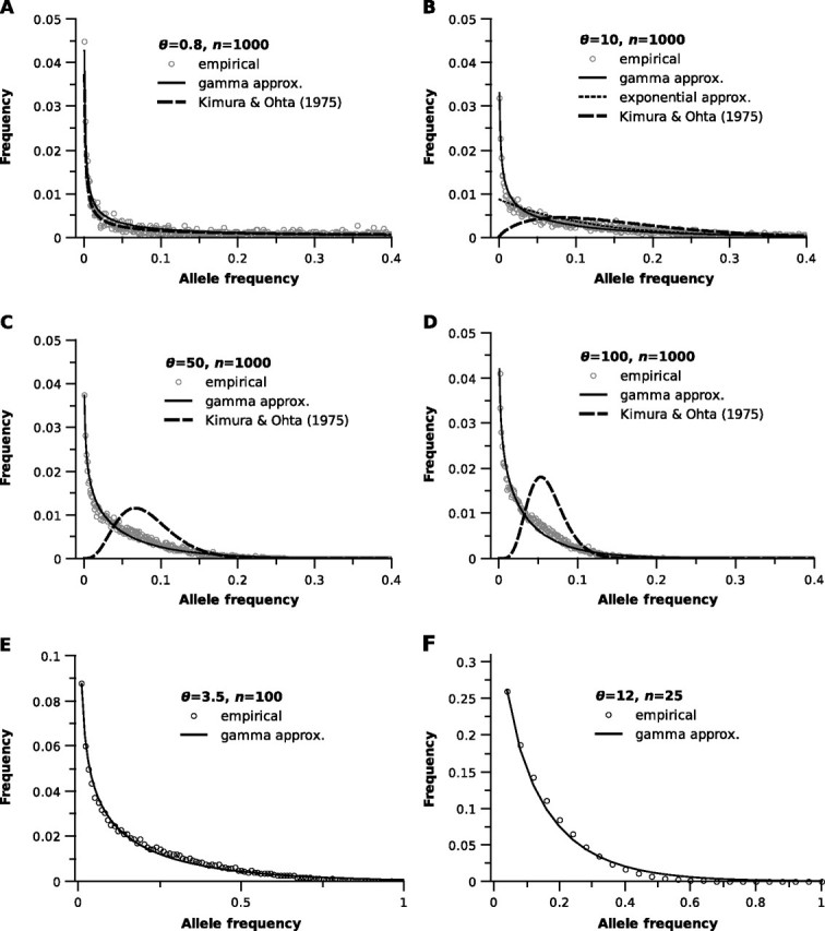
The microsatellite allele frequency spectrum. Simulated frequency spectra (open dots) compared with the gamma approximation of the frequency spectrum (solid lines) and the frequency distribution specified by Kimura and Ohta (1975; dashed lines). θ and sample size, n, are listed in the legend of each panel. (B) only shows the exponential approximation (dotted line) for comparison. Note the changes in scale of the x and y axes in (E) and (F).

In search of a better fit to simulated spectra, we next tried the gamma distribution with density function

where $\Gamma \left(\alpha \right)$ is the gamma function, α and β are the shape and scale parameters, and $E\left(X\right)=\alpha /\beta$. Assuming a gamma distribution and using the definition of mean allele frequency, , the expected number of alleles (n_a) for a locus is equal to β/α:

(4a)

(4b)

and the microsatellite allele frequency spectrum with parameters α and n_a is approximated by

(5)

Furthermore, for a given value of θ, n_a may be approximated using the ratio of homozygosity to mean allele frequency:

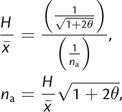(6)

where the expression for homozygosity (H) is taken from Kimura and Ohta (1975; eq. 3). Clearly, substituting for H reduces (6) to (4a). However, our goal was to express n_a as a function of θ. To this end, we plotted average versus $\text{ln}\left(\theta \right)$ using data sets simulated under a large number of θ values for $n=25$, $50,100,150,200,250,500,and1,000$ and performed curvilinear regression (fig. 2A; $10^6$ simulated data sets per point). For each value of n, the resulting curve described the ratio of interest as a function of θ and

(7)

where the coefficients $c_0,c_1$, and $c_2$ are specific to n and listed in supplementary table 1, Supplementary Material online. Figure 2B is based on the same simulated data as figure 2A; it plots E(n_a) versus θ for a variety of n. Independent simulations of n_a for a variety of θ and n confirmed that the curves based on (7) and depicted in figure 2B are predictive of E(n_a). Figure 2 also illustrates the intuitive result that fewer unique alleles are uncovered with each doubling of sample size. In particular, the $n=500$ and $n=1,000$ lines are nearly coincident. It follows that $n_{\text{a}(n=1,000)}\approx {\nu }_{\text{a}}$ for all values of θ simulated here, where ${\nu }_{\text{a}}$ is the number of alleles in the population rather than the sampled number of alleles.

FIG 2.

The microsatellite sampling distribution. (A) Average value of versus θ for seven different sample sizes. Each point represents the average of $10^6$ simulations. Dashed lines are second-order curvilinear regressions. (B) The expected number of alleles $E(n_a)$ versus θ for five different sample sizes. Curves were derived from the same simulated data as in (A), using the formula .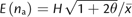

Finally, to express the microsatellite frequency spectrum as a function of θ only, it was necessary to find the relationship between θ and the shape parameter, α. Using (7) and the results of independent simulations, for each value of θ, we found the value of α that minimized the difference between the frequency of x=0.001 simulated alleles and the frequency predicted by the approximation. We then plotted the best values of α versus ln(θ) for a variety of n and fit a line with formula

(8)

Intercept a₀ is specific to n and listed in supplementary table 1, Supplementary Material online. A final formulation of the microsatellite frequency spectrum is obtained by applying n-specific versions of equations (7) and (8) to equation (5).

Next, we examined the correspondence between the gamma approximation to the frequency spectrum and empirical spectra. When multiplied by $\delta x=0.001$ (simulated spectra were generated using bins of this width when n=1,000), the gamma approximation of the microsatellite frequency spectrum provided excellent fit to frequency spectra simulated with n=1,000 (fig. 1A–D, solid lines). We also observed good agreement between the gamma approximation and empirical spectra for other sample sizes (fig. 1E, n=100 and fig. 1F, n=25). For comparison, the distribution specified by equation (15) of Kimura and Ohta (1975) fit the simulated data poorly for large values of θ (fig. 1, dashed lines). It is important to emphasize that the spectra shown in figure 1 are expected forms averaged over many thousands of homogeneous loci. As evident in figure 1A–D, a predominant feature of the microsatellite frequency spectrum is that the frequencies of low-frequency alleles increase greatly with θ, whereas alleles with frequencies >0.20 become extremely rare. One exception to this general trend is that very low θ values produce an abundance of the most rare alleles (allele frequencies ≤0.01; fig. 1A). Although the distributions presented in figure 1 do not integrate to exactly 1 on the interval $(0,1]$, they are very nearly 1 and are therefore good approximations of probability distributions. Finally, given frequency spectrum f(x), the probability that a randomly drawn allele will have a frequency on the interval [x, $x+\delta x$) is equal to $xf\left(x\right)\delta x$ (Ewens 1972). Plotting this quantity against allele frequency, using the gamma approximation for f(x), clearly demonstrates the effect of increasing θ on microsatellite variation (fig. 3).

FIG 3.

For three values of θ, plots of the expression $xf\left(x\right)\delta x$, which represents the probability that a randomly drawn allele will have a frequency in the interval [x, $x+\delta x$). Here, f(x) is our gamma approximation of the microsatellite allele frequency spectrum. The jaggedness of the plots at higher allele frequencies results when x is increasing but f(x) is the same for multiple, sequential values of x.

Estimation of θ Using the Number of AllelesSampled, n_a

Equation (7) may be used to compute the expected n_a for any value of θ. An observed n_a at a locus may then be matched to the most likely value of θ—an estimate that we refer to as . Although it seems self-evident to use the version of equation (7) specific to the actual sample size (fig. 2B; supplementary table 1, Supplementary Material online), we observed that this practice resulted in large inflated error (supplementary table 2, Supplementary Material online). An illustration of why this might be the case is presented in Supplementary figure 1, Supplementary Material online. Unfortunately, the identity of the best regression curve to use for estimation depends on the true value of θ (supplementary table 2, Supplementary Material online), which is obviously unknown in practice. We decided that the most practical course was to use the version of equation (7) specific to n = 1,000, which yields estimates relatively low in error regardless of n or θ. It is worth noting that the only estimates of θ possible are those that yield near-integer values when plugged into (7) because observed n_a is itself an integer. We also note that simulated values of n_a may be used to place confidence intervals on .

Estimation of θ Using the Vector of Sampled AlleleFrequencies, x

Given a value of θ, the probability of observing an allele frequency in the interval $(a,b]$ is found by taking the definite integral of $f_X\left(x\right)$, which is the exponential (3) or gamma (5) approximation to the frequency spectrum:

If 1) allele frequencies were independent, 2) sampled allele frequencies were the actual allele frequencies, and 3) the observed allele types were the only types present in the population, we could define the likelihood of observed allele counts as multinomial

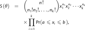(9)

where k is the number of alleles sampled, x_i is the frequency of the ith allele, and n_i is the count of the ith allele. Clearly, none of the three assumptions hold for real samples, and S(θ) is therefore not the likelihood of observed allele counts. However, we suspected this statistic might still be useful in the estimation of θ because it directly incorporates knowledge of the frequency spectrum. The interval of integration defined by a and b was centered on the observed frequency with width 1/n. This interval reflects the fact that observed allele frequencies are necessarily multiples of 1/n.

The frequency spectrum–based estimate () was identified by employing (9) in a grid search of potential θ values. was simply the θ value that maximized S(θ). In this maximization procedure, the multinomial coefficient in (9) is a constant for each value of θ tested and may be ignored. Thus, S(θ) in this context is more simply expressed as:

(10)

We used both approximations to the frequency spectrum to estimate θ in this way. Despite its relatively poor fit to simulated spectra, we found that the exponential approximation (3) produced more accurate estimates and therefore only report values of specific to the exponential approximation, which we refer to more specifically as . An illustration of why use of the exponential approximation may yield slightly better performance is presented in Supplementary figure 2, Supplementary Material online.

Estimation of θ Using the Mean of Sampled AlleleFrequencies,

Replacing the quadratic portion of equation (7) with a constant value of 2, and using the identity in (4a), we solved (7) for θ to obtain an estimator in terms of mean allele frequency:

(11)

where is the mean of sampled allele frequencies and is the estimate obtained by simply supplying the observed value of . For a particular value of n, the constant value used is only exact for a specific value of θ. Despite the inaccuracy introduced by the use of this constant, fares well across a broad range of θ.

Estimation by n_a, x, and Compared with OtherEstimators

We compared the performance of , , and with a variety of existing estimators. 40,000 simulated data sets were generated for each combination of θ ($1,5,10,25,50,75$, and 100) and n ($25,50,100,150,200$, and 250). In addition to , we estimated θ for each data set using , , and a form of the homozygosity estimator reported to correct its bias (; Xu and Fu 2004, eqs. 7 and 8). We also estimated θ on the first 150 simulated data sets for a smaller set of θ values using a product of approximate conditionals (PAC) approach (RoyChoudhury and Stephens 2007) and the full-likelihood Markov chain Monte Carlo approach implemented in MIGRATE (Beerli and Felsenstein 2001). PAC () and MIGRATE () estimates were obtained using default settings with the following exceptions: 1) was the average estimate across ten permutations, rather than one, and 2) in response to the observation that MIGRATE was performing poorly on data sets with high θ and/or n, burn-in was increased to 10,000 and the number of short and long chains was increased to 100 and 25, respectively, for all MIGRATE runs. Comparisons between , , and were based on 150 simulated data sets due to the greater run time required to obtain MIGRATE and PAC estimates. Finally, results indicated that and exhibited biases that were roughly equivalent in magnitude but opposite in sign. Therefore, we also made comparisons to an estimator that was simply the average of and : .

For each estimation method and each tested combination of θ and n, we used the i estimates to calculate Var(), bias

and MSE

To eliminate the possibility that our formulation of the microsatellite frequency spectrum was specific to our simulation algorithm, we performed many of the same comparisons using test data sets generated with the program ms and the accessory program microsat (Hudson 2002). This alternative approach produced nearly identical results. Additionally, forward-in-time simulations ($2N_{\text{e}}=10,000$) starting with an invariant microsatellite locus produced equilibrium values of ν_a for each tested value of θ near identical to those expected under (7), n=1,000 (data not shown).

, , and consistently underestimated the true value of θ by roughly equivalent amounts (table 1). In the case of small n and large θ, this bias was very large: as much as −78% of true θ for at θ=100 and n=25. With the exception of , at higher θ values, the lowest observed MSE of each estimator occurred when n≤150 (table 1). Again, results in supplementary table 2, Supplementary Material online indicate that an optimal version of (7) exists but depends on the true value of θ and n. Because users of our methods would not know the true value of θ, we reiterate our choice to only present results that use the n=1,000 version of (7). This is a safe choice, particularly for n≤250, but does not always produce the best possible performance (supplementary table 2, Supplementary Material online).

Table 1.

MSE and (Bias) of Six θ Estimators for a Variety of θ Values and Sample Sizes (n). Results Presented in Each Row Are Based on 40,000 Simulated Data Sets.

θ	n
1	25	0.58 (−0.48)	0.52 (−0.45)	0.58 (−0.48)	1.40 (−0.05)	3.46 (0.63)	1.12 (−0.02)
	50	0.60 (−0.20)	0.58 (−0.18)	0.57 (−0.31)	1.91 (0.09)	2.79 (0.60)	1.09 (0.03)
	100	0.66 (−0.08)	0.66 (−0.06)	0.62 (−0.18)	1.57 (0.01)	2.52 (0.58)	1.06 (0.05)
	150	0.73 (0.03)	0.75 (0.04)	0.65 (−0.14)	1.78 (0.06)	2.57 (0.61)	1.10 (0.08)
	200	0.77 (0.09)	0.80 (0.10)	0.66 (−0.14)	1.64 (0.03)	2.41 (0.56)	1.05 (0.05)
	250	0.78 (0.09)	0.81 (0.10)	0.68 (−0.11)	1.56 (0.00)	2.40 (0.57)	1.05 (0.05)
	500	0.75 (0.10)	0.84 (0.11)	0.69 (−0.07)	1.67 (−0.01)	2.36 (0.55)	1.05 (0.04)
	1,000	0.84 (0.20)	0.95 (0.21)	0.74 (−0.01)	1.68 (0.00)	2.32 (0.55)	1.05 (0.05)
5	25	7.63 (−2.19)	7.66 (−2.10)	8.35 (−2.23)	39.26 (0.12)	38.69 (2.26)	15.34 (−0.17)
	50	6.34 (−1.38)	6.79 (−1.24)	7.11 (−1.31)	32.09 (−0.11)	27.76 (1.89)	13.64 (−0.03)
	100	6.35 (−0.72)	7.45 (−0.51)	7.62 (−0.60)	36.31 (0.03)	23.73 (1.77)	12.90 (0.06)
	150	6.66 (−0.36)	8.22 (−0.12)	7.89 (−0.35)	36.25 (0.04)	21.70 (1.68)	12.72 (0.04)
	200	6.70 (−0.30)	8.28 (−0.05)	8.38 (−0.22)	32.98 (−0.11)	21.62 (1.68)	12.26 (0.07)
	250	7.30 (−0.11)	9.29 (0.17)	8.65 (−0.15)	32.58 (−0.12)	21.04 (1.60)	12.12 (0.02)
	500	7.60 (0.06)	11.78 (0.71)	9.95 (0.27)	36.3 (0.08)	21.01 (1.68)	12.11 (0.11)
	1,000	8.34 (0.30)	13.33 (0.99)	10.79 (0.48)	35.37 (−0.01)	20.18 (1.57)	11.81 (0.04)
10	25	32.59 (−5.07)	31.68 (−4.80)	32.12 (−4.86)	165.44 (0.25)	142.75 (4.44)	55.97 (−0.20)
	50	23.42 (−3.47)	24.23 (−2.98)	24.46 (−3.03)	136.10 (−0.12)	85.93 (3.22)	44.80 (−0.15)
	100	21.18 (−2.13)	25.70 (−1.41)	24.95 (−1.42)	160.60 (0.27)	72.54 (3.01)	41.26 (0.07)
	150	20.84 (−1.46)	27.45 (−0.61)	26.22 (−0.98)	136.33 (0.04)	66.18 (2.74)	39.16 (−0.04)
	200	21.62 (−1.15)	29.80 (−0.24)	27.85 (−0.67)	128.24 (−0.13)	64.86 (2.69)	38.80 (−0.02)
	250	22.58 (−0.82)	32.43 (0.15)	28.68 (−0.27)	131.27 (0.01)	63.58 (2.77)	37.94 (0.07)
	500	22.92 (−0.66)	37.99 (1.04)	33.26 (0.38)	130.66 (−0.05)	59.94 (2.61)	36.6 (0.00)
	1,000	24.72 (−0.14)	43.79 (1.70)	36.86 (0.90)	137.53 (0.03)	60.40 (2.60)	37.17 (0.02)
25	25	260.33 (−15.58)	238.67 (−14.59)	234.44 (−14.43)	903.13 (−0.51)	963.32 (11.19)	370.38 (−0.16)
	50	163.59 (−11.14)	146.18 (−9.09)	145.48 (−9.19)	867.12 (0.06)	489.12 (7.71)	256.98 (−0.03)
	100	124.27 (−7.50)	134.25 (−4.42)	128.80 (−4.88)	938.10 (0.48)	371.22 (6.47)	216.67 (0.03)
	150	114.45 (−6.08)	138.76 (−2.57)	138.17 (−3.07)	728.61 (−0.78)	342.89 (6.22)	205.18 (0.12)
	200	113.71 (−5.14)	151.87 (−1.34)	144.97 (−2.31)	759.54 (−0.70)	319.68 (5.74)	196.06 (−0.13)
	250	113.93 (−4.53)	161.29 (−0.55)	152.06 (−1.34)	716.11 (−0.94)	310.82 (5.70)	191.16 (−0.08)
	500	118.14 (−3.67)	200.4 (1.92)	188.00 (0.88)	803.3 (−0.16)	291.44 (5.44)	182.27 (−0.15)
	1,000	122.70 (−2.57)	231.52 (3.42)	210.54 (2.12)	837.15 (−0.04)	288.20 (5.38)	181.82 (−0.13)
50	25	1,276 (−35.26)	1,143 (−33.02)	1,144 (−33.02)	3,393 (−1.18)	4,859 (24.94)	1,712 (1.56)
	50	814.2 (−22.04)	650.2 (−22.04)	646.6 (−21.99)	3,412 (−0.53)	1,955 (15.20)	1,040 (0.35)
	100	544.0 (−18.87)	464.1 (0.14)	480.7 (−12.08)	3,282 (0.14)	1,380 (12.28)	819.9 (0.14)
	150	473.8 (−15.32)	468.6 (−6.75)	491.9 (−7.93)	2,875 (−1.08)	1,195 (10.97)	732.2 (−0.34)
	200	460.3 (−13.17)	521.4 (−3.91)	525.6 (−5.34)	3,286 (−0.45)	1,185 (11.13)	733.7 (0.07)
	250	438.9 (−11.66)	537.9 (−1.90)	557.9 (−3.56)	2,810 (−1.90)	1,126 (10.61)	704.2 (−0.20)
	500	442.4 (−10.17)	719.2 (2.92)	740.5 (2.15)	2,991.4 (−1.15)	1,039.2 (9.85)	663.2 (−0.53)
	1,000	452.2 (−7.62)	880.2 (6.62)	867.0 (5.23)	3,114.5 (−0.32)	1,009.8 (9.57)	651.0 (−0.62)
75	25	3,253 (−56.65)	2,926 (−53.59)	2,901 (−53.16)	6,258 (−2.33)	12,403 (40.05)	4,243 (4.26)
	50	2,063 (−43.77)	1,582 (−36.35)	1,603 (−36.47)	6,702 (−1.95)	4,415 (23.08)	2,349 (1.11)
	100	1,372 (−32.18)	1,032 (−20.95)	1,070 (−20.88)	6,685 (−1.86)	2,963 (17.65)	1,776 (−0.04)
	150	1,144 (−26.32)	963.6 (−13.19)	1,043 (−13.37)	6,097 (−2.69)	2,685 (16.67)	1,652 (0.06)
	200	1,058 (−22.70)	1,014 (−8.41)	1,106 (−9.36)	5,896 (−2.48)	2,512 (16.05)	1,966 (−0.03)
	250	1,010 (−20.38)	1,061 (−5.35)	1,178 (−6.08)	6,154 (−2.06)	2,445 (15.72)	1,537 (−0.06)
	500	1,001 (−17.6)	1,560 (3.69)	1,730 (4.08)	6,914 (−1.61)	2,251 (14.01)	1,456 (−1.03)
	1,000	987 (−13.56)	1,917 (9.76)	2,044 (9.32)	6,873 (−1.17)	2,158 (13.80)	1,402 (−0.99)
100	25	6,229 (−78.58)	5,627 (−74.38)	5,673 (−74.72)	10,463 (−4.52)	29,701 (54.50)	7,916 (5.63)
	50	4,052 (−62.00)	3,108 (−52.32)	3,155 (−52.07)	11,132 (−2.91)	7,295 (30.00)	4,207 (1.13)
	100	2,614 (−46.03)	1,834 (−31.18)	1,918 (−30.66)	10,536 (−4.08)	5,091 (22.38)	3,088 (−0.66)
	150	2,116 (−37.60)	1,616 (−20.10)	1,820 (−20.36)	9,971 (−3.81)	4,484 (20.31)	2,805 (−1.18)
	200	1,936 (−32.84)	1,664 (−13.86)	1,900 (−13.90)	10,582 (−4.37)	4,391 (20.54)	2,765 (−0.43)
	250	1,829 (−28.81)	1,782 (−8.59)	2,024 (−9.51)	11,080 (−2.27)	4,237 (19.86)	2,688 (−0.68)
	500	1,782 (−25.50)	2,684 (4.55)	3,213 (7.06)	10,372 (−3.74)	3,298 (18.70)	2,543 (−1.05)
	1,000	1,755 (−19.48)	3,475 (13.76)	3,998 (15.26)	11,257 (−1.50)	3,829 (18.55)	2,490 (−0.88)

Note.—Values in italic indicate the lowest MSE achieved by any estimate for a particular value of θ.

Assuming the n=1,000 version of (7) is used, all three of our estimators are statistically inconsistent: their variances increase with sample size. We explored the possibility that subsampling might yield statistically consistent estimates. Specifically, for n≤250, we generated 100 random subsamples of n=100 each, estimated θ on each of the subsamples, and retained the average of these estimates as the final estimate. This method can lead to significant improvements in MSE for our estimators (supplementary table 3, Supplementary Material online). However, whether or not MSE is improved by the subsampling method is again dependent on the (unknown) true value of θ. For large values of θ, subsampling can in fact lead to large increases in MSE of (supplementary table 3, Supplementary Material online).

Despite statistical inconsistency and large bias when n was small, all three of our proposed estimators exhibited much lower MSE than , , or (table 1). and produced nearly identical results across all combinations of θ and n. exhibited somewhat different behavior, frequently achieving the lowest MSE of any estimator listed in table 1 (italic) and demonstrating a less rapid decay of variance with increasing sample size. Of the remaining three estimators presented in table 1, exhibited the lowest MSE. As reported previously (Xu and Fu 2004), this estimator corrects the bias of , though it does begin to exhibit minor bias when θ≥50 and n≤50. and exhibit extraordinary error when θ is large and appears truly biased as its decline in bias seems to plateau at n≤150 (table 1).

For θ=5 and regardless of n, also exhibited lower MSE than or (table 2). For $\theta =10,50,100$ and n≤100, showed lower MSE than , whereas for n≤100, exhibited comparable MSE to that of and (table 2). As mentioned above, and exhibited roughly symmetrical biases. The performance of both estimators was frequently improved considerably by averaging them. For many combinations of θ and n, showed less (sometimes substantially so) MSE that any individual estimation method (table 2). It is worth noting that although and also share symmetrical biases (table 1), the average of their estimates did not result in decreased MSE.

Table 2.

MSE and (Bias) of Four θ Estimators for a Variety of θ Values and Sample Sizes (n). Results Presented in Each Row Are Based on 150 Simulated Data Sets.

θ	n
5	25	8.39 (−1.96)	26.05 (1.43)	23.3 (1.10)	12.03 (−0.27)
	50	5.85 (−0.88)	15.31 (1.57)	9.17 (−0.10)	7.97 (0.35)
	100	7.31 (−0.19)	8.93 (0.98)	13.68 (0.87)	7.09 (0.40)
	150	7.42 (−0.13)	7.94 (0.69)	14.21 (1.69)	6.77 (0.28)
	200	7.94 (−0.09)	8.45 (0.62)	13.85 (0.89)	6.42 (0.27)
	250	8.40 (0.20)	9.38 (0.82)	16.96 (1.47)	7.84 (0.51)
10	25	34.03 (−5.03)	66.32 (1.4)	52.46 (0.82)	31.97 (−1.82)
	50	24.46 (−2.95)	45.41 (1.64)	32.25 (−0.04)	25.72 (−0.66)
	100	25.64 (−1.03)	37.16 (2.09)	37.82 (1.05)	23.16 (0.10)
	150	31.87 (−0.78)	27.70 (0.76)	23.94 (0.49)	24.41 (−0.01)
	200	29.33 (0.55)	18.50 (0.15)	19.83 (0.20)	20.70 (−0.20)
	250	25.45 (0.49)	20.36 (0.57)	30.3 (1.07)	19.46 (0.04)
50	25	1,114.74 (−32.49)	1,712.82 (13.51)	488.7 (−14.09)	607.43 (−9.49)
	50	649.48 (−21.03)	968.20 (8.06)	430.64 (−11.21)	487.37 (−6.48)
	100	408.12 (−11.97)	476.20 (4.38)	400.5 (−10.27)	316.02 (−3.79)
	150	560.78 (−4.52)	577.09 (6.90)	357.0 (−9.50)	462.54 (1.91)
	200	533.72 (−3.83)	330.28 (0.66)	377.03 (−8.98)	361.12 (−1.58)
	250	589.59 (0.94)	348.02 (4.26)	318.83 (−8.25)	369.25 (2.60)
100	25	5,831.24 (−75.84)	2,634.15 (3.88)	2,590.0 (−47.01)	2,144.69 (−35.98)
	50	2,976.69 (−51.15)	3,703.58 (21.75)	1,936.0 (−37.11)	1,546.09 (−14.70)
	100	1,805.86 (−31.91)	2,185.54 (11.69)	2,206.9 (−41.38)	1,215.98 (−10.10)
	150	1,548.14 (−18.04)	1,991.27 (10.52)	1,407.0 (−29.66)	1,293.62 (−3.76)
	200	1,564.57 (−17.18)	1,528.86 (1.52)	1,641.5 (−32.87)	1,218.80 (−8.15)
	250	1,442.96 (−11.61)	1,240.68 (3.74)	1,404.3 (−29.08)	970.37 (−3.94)

Multistep Mutation and θ Estimation

The evolution of many microsatellite loci likely includes multistep mutations, a violation of a key SMM assumption (DiRienzo et al. 1994). It was therefore important to determine how multistep mutation affected , , and in comparison to other estimators. Under the generalized stepwise model (GSM), microsatellite mutations are still Poisson distributed, but mutations of >1 step are allowed. One-hundred and fifty data sets of θ=10 and n=25 or 250 were simulated following a GSM. Step size was drawn from a geometric distribution with parameter $P=0.63$, which specifies the probability of a single-step mutation. Although data suggest P is greater than 0.63 for most loci (DiRienzo et al. 1994, Dib et al. 1996), we chose a small value of P in order to ensure frequent multistep mutations and clear departure from SMM evolution. As expected, data sets modeled under the GSM produced estimates with greater MSE and larger positive bias than did comparable SMM data sets (table 3). and were least affected for n=50 and n=250, respectively. The change in mutational model had the greatest effect on (table 3). Although MSE for was 1.5 and 9.5 times greater under the GSM than under the SMM for n=50 and 250, respectively, MSE increased by >30 times regardless of sample size.

Table 3.

Effects of Multistep Mutations on θ Estimation. MSE based on 10,000 Independent Estimates (θ=10 and n=50, 250), Except for and Based on 150 Independent Estimates. Data Sets Were Modeled Assuming the GSM with Probability of a Single-Step Mutation, P = 0.63. Values from SMM Simulations Are Taken from Tables 1 and 2 and Listed for Comparison

	n = 50		n = 250
Method	GSM	SMM	GSM	SMM
	34.8	23.4	213.5	22.6
	61.2	24.2	388.9	32.4
	60.2	24.4	284.62	28.7
	4,740.0	136.1	4,265.1	131.3
	390.4	85.9	302.5	63.6
	163.9	44.8	156.4	37.9
	416.0	45.4	148.5	20.7
	180.8	32.3	104.7	30.3

Demographic Change and θ Estimation

We were interested in quantifying the effect of nonequilibrium conditions on all θ estimators. We employed a model of demographic change in which a population undergoes an instantaneous bottleneck followed by an exponential growth until the present. Four parameters characterize this model (fig. 4): t_b, the time of the bottleneck; r, the rate of exponential growth; N₀, the current census population size; and N_a, the prebottleneck census population size. During the period of exponential growth, the size of the population $g\times 4N_0$ generations ago is specified by the equation $N\left(g\right)=N_0{\text{e}}^{-rg}$. This general demographic scenario is commonly modeled because it likely captures the population dynamics exhibited by numerous species including humans (Slatkin and Hudson 1991).

FIG 4.

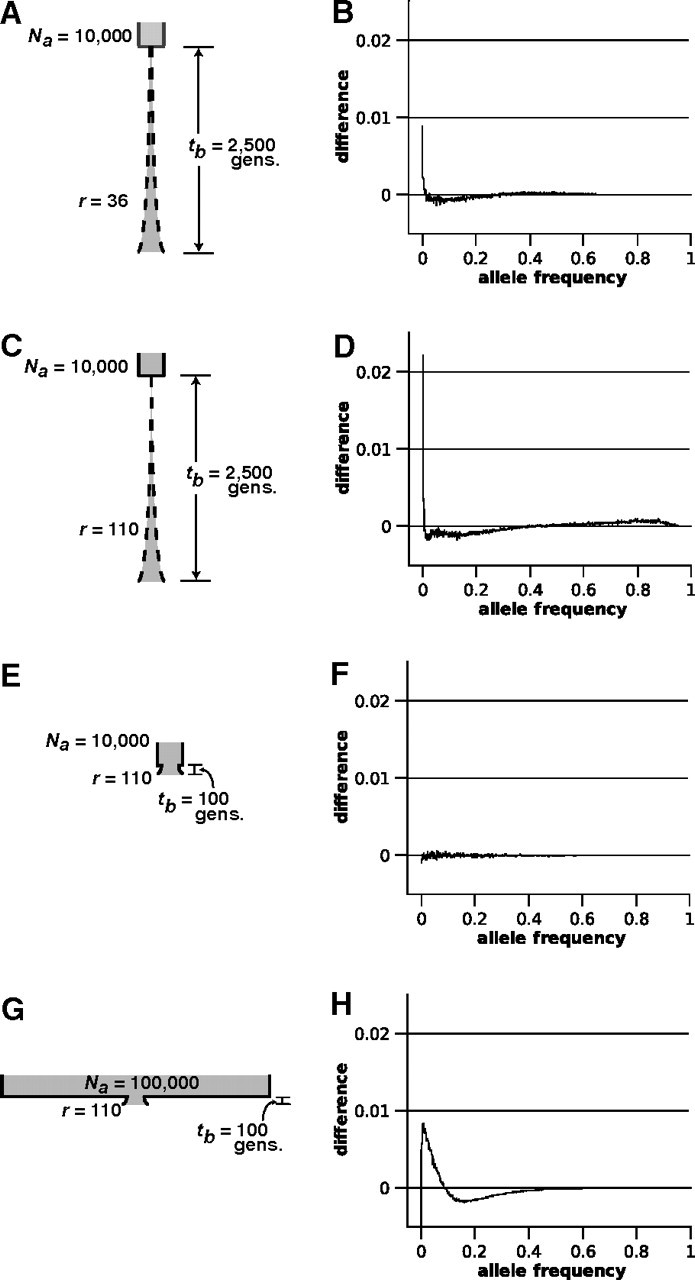
Effect of demographic change on the microsatellite frequency spectrum. The demographic scenario modeled (left column) and resulting change to the microsatellite frequency spectrum (right column) for scenarios I (A and B), II (C and D), III (E and F), and IV (G and H). Difference plotted on the y axis is the nonequilibrium spectrum minus the spectrum under constant population size. All spectra were each based on 10,000 simulations of $n=1,000$ data sets. N_a, ancestral census population size; r, rate of exponential growth; and t_b, number of generations ago when the bottleneck occurred.

We investigated four distinct instances of the bottleneck-expansion model (fig. 4A–D). In all four scenarios, $N_0=10,000$, $\mu =0.00025$, and present-day θ=10. In scenario I (sustained exponential growth, moderate bottleneck), $t_{\text{b}}=2,500\text{generations}$, $N_{\text{a}}=10,000$, and r=36 (fig. 4A). In scenario II (sustained exponential growth, severe bottleneck), $t_{\text{b}}=2,500\text{generations}$, $N_{\text{a}}=10,000$, and r=110 (fig. 4C). In scenario III (recent, mild bottleneck), $t_{\text{b}}=100\text{generations}$, $N_{\text{a}}=10,000$, and r=110 (fig. 4E). Finally, in scenario IV (recent bottleneck of intermediate strength), $t_{\text{b}}=100\text{generations}$, $N_{\text{a}}=100,000$, and r=110 (fig. 4G).

For each scenario, we calculated the inbreeding effective population size, $N_{\text{e}}^i$, using the formula , where t is the number of past generations examined. This accounting of the current effective population size incorporates past changes in census population size. For all scenarios, we set t=40,000, which was four times the current census population size. The true contemporary value of ${\theta }_{\text{T}}=4N_{\text{e}}^i\mu$ was then calculated for each scenario: 8.52, 1.03, 9.99, and 97.44 for scenarios I, II, III, and IV, respectively. Thus, the different demographic scenarios produced widely different effects on the true value of contemporary θ. If we consider that $4N_0\mu =10$ for all scenarios, we see that the contemporary θ was little affected by the small period of time during which $N<10,000$ under scenario III. Conversely, the large amount of time spent at $N=100,000$ under scenario IV increased contemporary θ dramatically despite much smaller values of N in recent generations.

To test the effect of demographic change on θ estimation, 150 data sets were produced (n=250) for each demographic scenario. We used ms (Hudson 2002) to simulate genealogies and a custom-written program to apply mutation. PAC and MIGRATE run conditions were the same as above. In all cases, MSE and bias were calculated by comparing estimated θ to the values of θ_T calculated above. In general, MSE and bias associated with estimates of θ_T were similar to those observed when a true θ of similar magnitude was estimated under a model of constant population size (table 4). In fact, in many cases, it appeared that MSE actually improved under scenarios of demographic change (e.g., compare table 4 scenario I results with those for $\theta =1.0$, n=250 in table 1), although this may simply result from sampling error; the results in table 4 are based on 150 replicates, whereas those in table 1 are based on 40,000 replicates.

Table 4.

Demographic Change and θ Estimation. MSE and Bias (in parentheses) Are Shown. The Scenarios Refer to the Histories of Bottleneck Followed by Expansion Shown in Figure 4. All Statistics, Except for Those Associated with Constant Population Size, Are Based on Estimates from 150 Independent Data Sets. Constant Population Size Statistics (θ=10) Are Drawn from Tables 1 and 2. θ_T is the True Value of $\theta =4N_{\text{e}}^i\mu$, Where $N_{\text{e}}^i$ Was Calculated Based on the Fluctuating Census Population Size of the Past 40,000 Generations

Model	θT
Scenario I	8.52	19.4 (−3.2)	19.8 (−2.5)	20.5 (−2.9)	198.6 (−0.2)	26.4 (−2.3)	28.3 (−3.8)	14.8 (−2.4)	10.6 (−1.6)
Scenario II	1.03	0.69 (0.4)	0.84 (0.4)	0.51 (0.2)	0.34 (−0.4)	0.96 (0.1)	0.62 (−0.3)	1.38 (0.7)	5.99 (2.1)
Scenario III	9.99	20.0 (−1.4)	29.2 (0.11)	27.3 (−0.4)	87.3 (−0.6)	67.2 (2.6)	41.3 (−0.1)	27.7 (1.5)	36.7 (0.7)
Scenario IV	97.4	1,879 (−36.0)	1,453 (−12.9)	1,589 (−9.8)	8,545 (1.8)	3,007 (10.3)	2,059 (−8.4)	1,111.8 (4.8)	1,500 (−31.1)
Constant size	10.0	22.6 (−0.8)	32.4 (+0.2)	28.7 (−0.3)	131 (0.0)	63.6 (+2.8)	37.9 (+0.1)	20.4 (0.6)	30.3 (1.1)

Demographic Change and the Frequency Spectrum

We also conducted a preliminary examination of the effect of demographic change on the frequency spectrum. Using the same scenarios specified in the Demographic Change and θ Estimation section, 10,000 independent loci (n=1,000) were simulated for each of the four scenarios. As with the constant population size model, the resulting data were pooled to form empirical frequency spectra. We examined deflections of the frequency spectrum due to demographic change by comparing nonequilibrium spectra to the spectrum expected when population size is constant and θ=10. We chose this as the null spectrum because for all scenarios of demographic change modeled here, $4N_0\mu =10$. Panels in the right-hand column of figure 4 plot the average differences between the nonequilibrium and constant population size (θ=10) spectra for each of the four scenarios. Under scenarios I and II, sustained exponential growth had the effect of increasing the frequency of very rare alleles (allele frequency <0.01) and decreasing the frequency of intermediate frequency alleles ($0.01<\text{allele\hspace{0.5em}frequency}<0.30$). Both these trends were more pronounced in the case of the more severe bottleneck (scenario II; fig. 4D). Additionally, the increased rate of exponential growth in scenario II was associated with a noticeable increase in the frequency of high-frequency alleles (allele frequency >0.60; fig. 4D). The amplitude of this high-frequency peak increased with r and became very pronounced between allele frequencies of 0.90 and 0.99 when r=1,000 (data not shown). No difference was detected between the spectrum under the constant population size model and the spectrum under scenario III (fig. 4F), despite the recent 25% reduction in population size. The more severe bottleneck of scenario IV, however, produced a decline in singleton alleles (allele frequency =0.001), a dramatic increase in the frequency of rare-to-intermediate alleles (0.001< allele frequency <0.1), and a decline in intermediate-to-common alleles (0.1< allele frequency <0.5; fig. 4H).

We calculated three summary statistics for each of the simulated data sets: 1) n_a; 2) range, the lowest frequency subtracted from the highest frequency; and 3) rarest fraction, the fraction of alleles with frequencies <0.05 that are also <0.01 (e.g., for observed frequencies 0.90, 0.03, 0.02, 0.02, 0.015, 0.005, 0.005, and 0.005, rarest fraction is 3/7). Based on the observed changes to the frequency spectrum depicted in figure 4, we suspected the latter two statistics held potential to diagnose demographic history. The average values of the three statistics are listed in table 5.

As figure 1 and Supplementary figure 2, Supplementary Material online make clear, changes to θ alone cause deflections of the frequency spectrum. However, in some circumstances, it may be possible to detect unusual deflections of the frequency spectrum associated with demographic change, such as the increase in abundance of high-frequency alleles under scenario II (fig. 4D). We recommend isolating deflections due to demographic change using the following simple procedure: 1) simulate data sets using a value of θ that produces an average n_a similar to that observed in the empirical data set, 2) calculate the average range and rarest fraction from the simulated data, and 3) check for discrepancies between the simulation summaries and those calculated from the observed data set. As an example, consider scenarios II and IV for which we provide average values of summary statistics from data sets simulated with constant population size and values of θ that produced n_a comparable to those under nonequilibrium conditions (table 5). For scenario IV (strong and recent bottleneck), the average values of all three summary statistics were similar to those of data simulated with θ=89.5 and constant population size (table 5). On the other hand, despite similarity in n_a, the average frequency range of scenario II data sets was quite different from that of data sets simulated with θ=1.5 and constant population size (table 5).

Table 5.

Demographic Change and the Frequency Spectrum. Range Is the Highest Frequency Minus the Lowest Frequency. Rarest Fraction is the Fraction of Alleles with Frequencies ≤0.05 that Are also ≤0.01. All Statistics Listed Are Averaged Across 10,000 Independent Simulations.

Model	na	Range	Rarest Fraction
Scenario I	7.40	0.43	0.45
Scenario II	4.38	0.71	0.50
Constant size (θ= 1.5)	4.25	0.59	0.46
Scenario III	9.06	0.32	0.40
Scenario IV	23.72	0.14	0.31
Constant size (θ= 89.5)	24.12	0.13	0.35

Discussion

The Microsatellite Allele Frequency Spectrum

Though the distribution of allele types at microsatellite loci evolving under the SMM has been investigated in great analytical detail (Moran 1975, wehrhahn75, Brown et al. 1975, Weir et al. 1976, Chakraborty and Nei 1982, Beder 1988), the distribution of allele frequencies has received less attention. The only available formula for the microsatellite frequency spectrum was derived under assumptions that limit its application to microsatellite loci with very low mutation rates (Kimura and Ohta 1975, Kimura and Ohta 1978). We used coalescent simulation to develop gamma and exponential approximations to the microsatellite allele frequency spectrum under the SMM. Whether exponential or gamma, the parameter of biological relevance was n_a, which can be expressed in terms of θ.

A visual comparison of results from different θ values in figures 1A–D and 3 as well as Supplementary figure 2, Supplementary Material online demonstrates the predictable effect of θ on microsatellite variation: as θ increases, low-frequency alleles become very frequent and intermediate- to high-frequency alleles become very rare. Though intuitive, this result is in direct contrast to the unfolded SNP spectrum in which the ratio of rare to common alleles remains unchanged as θ increases (Fu 1995). This fundamental difference between microsatellite and SNP spectra stems from the different definitions of SNP and microsatellite polymorphism. Individual SNPs are defined as biallelic under the infinite alleles and infinite sites models. As such, SNP θ affects the number of SNPs and not the number of alleles at individual SNP loci. The frequencies of derived alleles, in this case, are mainly a function of age (Kimura and Ohta 1973) and the time of introduction of neutral SNPs is random. These facts ensure that the relative proportions of SNP allele frequencies found in the population remain unchanged by θ (Fu 1995). On the other hand, an individual microsatellite is likely to possess a large number of alleles. As microsatellite θ increases, density on the frequency spectrum begins to pile up at low frequencies due to increasing number of alleles and their decreasing frequencies.

Comparison of Microsatellite θ Estimators

No estimator compared in our study is superior under all conditions. For example, though clearly provides the best performance when θ=50, it frequently requires long (though not prohibitive) computation time and is consistently outperformed by when θ=5 (table 2). Although under all conditions our three estimators clearly exhibit less error than the others presented in table 1, offers variable competitiveness with and (table 2). Also, although the estimates , , and demonstrate largely similar diagnostic statistics, they frequently exhibit their lowest MSE at different sample sizes when the default n=1,000 regression is used (table 1). It is again worth noting that both the use of other regressions in equation (7) (supplementary table 2, Supplementary Material online) and subsampling (supplementary table 3, Supplementary Material online) have great potential to improve the accuracy of our estimators. However, this will be difficult to do in practice because the efficacy of both these alternate methods is dependent on θ. Nevertheless, if very high values of θ (>50) can be ruled out, it appears that subsampling is safe and highly effective in the cases of and (supplementary table 3, Supplementary Material online).

We often found that when all estimates based on a single data set were compared, the outlier estimate was the most accurate. This fact discourages the practice of taking the average of all estimates or discarding outlier estimates. An exception to this rule is , which is the average of and estimates. More often than not, demonstrated lower MSE than all other estimators (table 2). On average, we suggest this compound estimator is the best option for θ estimation when no a priori information is available regarding the locus in question and n≥100. We note, however, that appears to do well merely by the coincidence of opposite biases and we do not imply any underlying biological meaning for the good performance of this estimator.

Ewens (1972) showed that the sampled number of alleles was a sufficient statistic for SNP θ and that allele frequencies provided no further information in this regard. In an interesting parallel to this finding, the MSE and bias of and are very similar across the range of θ values tested (table 1). Recall that is based on n_a alone, whereas is based on the number of alleles and their frequencies. Although we make no theoretical claim that n_a is a sufficient statistic for microsatellite θ, our results do suggest that estimation of microsatellite θ is similarly unimproved by allele frequency information.

As noted by RoyChoudhury and Stephens (2007), consistently outperforms the other moment estimator, (table 1). Estimator , a regression corrected form of (Xu and Fu 2004), generally performed well in terms of MSE and bias (table 1). However, we found that this reportedly unbiased estimator began to exhibit some bias for θ≥50. The largest value of θ tested by Xu and Fu (2004) was 40, suggesting that their regression equations are less applicable to loci with very large θ whenever n is small. In conjunction with the fact that the unbiased estimator began to demonstrate appreciable bias when θ≥75 (table 1), this result emphasizes that new methods should be tested across a wide range of biologically realistic parameter values.

The bias of , , and

When sample size is small, an individual sample of allele frequencies, x, is likely to diverge greatly from the expected frequency spectrum. For example, as θ increases, the number of alleles with frequencies <0.01 increases (figs. 1 and 4), but many of these alleles may fail to be surveyed in small samples. Similarly, the high sampling variance associated with small sample size implies greater divergence between n_a and $E(n_{\text{a}}$) as sample size decreases. Such discrepancies lead to extreme biases in the estimates , , and for sample sizes <100, especially when θ is very large (≥50; table 1). When using the n=1,000 regression, the biases are negative for small actual n because failure to detect rare alleles 1) flattens the sampled distribution of allele frequencies, making it more similar to low θ spectra and 2) frequently produces an allele count that is more in keeping with lower values of θ. The switch in sign of the bias sometimes observed as n increases (table 1, and ) or the version of equation (7) used changes (supplementary table 2, Supplementary Material online) signals that a version of equation (7) associated with zero bias exists for any situation. However, our results indicate that the interrelationship of n and θ is quite complicated and that use of the $n=1,000$ regression is the best default practice.

A rather remarkable result is that the estimation methods presented here and based on simple summaries of the data perform competitively even when sample size is much smaller than 1,000. Despite bias, our results indicate that n≤100 is frequently sufficient to achieve estimates with comparable or lower error than those of other estimators. In fact, sample sizes of this order frequently yield the most accurate estimates. Thus, these estimators represent fast, accurate means of estimating θ: they always outperform other “fast” estimates in table 1 and frequently outperform the more computationally intensive methods in table 2. The possibility remains that similar approaches may lead to estimators with less bias. For example, an estimator that matches observed n_a to the expected mode of n_a rather than mean n_a (eq. 7) might prove more robust to the technical complications detailed in Supplementary figure 1, Supplementary Material online.

Although ideal estimators are unbiased, MSE comprises variance and bias, which implies that low variance can lead to relatively small MSE despite high bias (Futschik and Gach 2008). Furthermore, MSE arguably has greater practical importance than other estimator diagnostics. For example, an unbiased estimator of θ with high MSE is only advantageous if a large number of loci known to be evolving identically are available. Only then will the average estimate approach the true value of θ at the homogeneous loci. Each estimate provided by a biased estimator with low MSE, on the other hand, will be relatively close to the true value of θ though less likely to be exactly correct. Similarly, ideal estimators are consistent. However, the range of sample sizes under which our estimators do the best overlaps the size of most empirical microsatellite data.

Multistep Mutation and θ Estimation

Multistep mutations may occur frequently in microsatellite evolution (DiRienzo et al. 1994). A concern regarding estimators explicitly built upon the single-step SMM (including all of those presented in table 1) is that multistep mutations will compromise their ability to estimate θ. This concern is certainly realized in the case of , where MSE increased by more than 30 times in response to the introduction of frequent multistep mutation (table 3). Other estimators, including and , also exhibited dramatically increased MSE in response to GSM evolution. The relative insensitivity of , , and to multistep mutation when n=50 is most likely another consequence of the inability of small data sets to detect rare alleles. Failure to detect the abundance of rare alleles produced by multistep mutation when n is small buffers and against the inflationary effect GSM evolution has on estimates of θ. Increased sample size eliminates this buffer and MSE, for example, is nearly 10-fold higher under the GSM than under the SMM, though absolute MSE is still comparable to other estimators (table 3).

Demographic Change and θ Estimation

The performances of all estimators were unaffected by the shift from a model of constant population size to models of recent demographic change (table 4). We suspected that estimator performance might be affected by mutation-drift nonequilibrium. For example, our estimators were developed using simulations that assumed constant population size. Of course, all estimators do perform poorly if we substitute the current census population size ($N_0=10,000$ in this case) for $N_{\text{e}}$ and thereby treat θ=10 as the true contemporary value of θ for all scenarios modeled. However, when we use the inbreeding effective population size ($N_{\text{e}}^i$) to calculate θ_T, expressions such as those in equations (1) and (2) still hold and estimators retain their relative abilities to estimate θ_T. Essentially, the use of $N_{\text{e}}^i$ averages fluctuations in mutational pressure associated with past expansions and contractions of population size across the genealogical depth of the locus.

Further Application of the Microsatellite Frequency Spectrum

Tests for departure from the neutral SNP frequency spectrum have enjoyed wide use in the inference of demographic parameters and detection of various forms of selection (e.g., Adams and Hudson 2004, Marth et al. 2004, Przeworski et al. 2005, Nielsen et al. 2009). In addition, summary statistics with direct relevance to the frequency spectrum—such as heterozygosity, number of alleles, range in allele size, and variance in allele size—have been employed in the detection of positive selection and analysis of historical demography using microsatellite data (Jorde et al. 1997, Kimmel et al. 1998, Luikart and Cornuet 1998, Wiehe 1998, Beaumont 1999, Garza and Williamson 2001, Payseur et al. 2002, Storz et al. 2004). Direct comparison of the full array of allele frequencies at multiple loci to the expected frequency spectrum might increase the sensitivity of such approaches. The gamma approximation to the allele frequency spectrum might also allow frequency spectra at microsatellites and SNPs to be combined by using a composite likelihood approach (Adams and Hudson 2004, Nielsen et al. 2005). Simultaneous use of both marker types could refine estimates of demographic and selection parameters. Of course, strong dependency of the spectrum on the actual value of θ makes its application in these other contexts somewhat challenging.

The frequency spectrum might also be usefully employed in methods of approximate Bayesian computation (ABC; Beaumont et al. 2002, Plagnol and Tavaré 2004), where posterior probabilities of parameters of interest are computed based on comparisons between summaries of observed and simulated data. Unfortunately, sufficient summary statistics are frequently unknown for the parameters of interest (Marjoram and Tavaré 2006). We suggest that simulations of the frequency spectrum under various evolutionary scenarios may inspire novel (though not necessarily sufficient) summary statistics for use in ABC. As an example, consider our simulations of four demographic scenarios (fig. 4). Three of the four scenarios led to distinct deflections of the frequency spectrum (fig. 4B, D, and H). In particular, scenario II—a severe bottleneck followed by extended exponential growth—produced an n_a in keeping with $\theta \sim 1.5$ (table 5). On average, however, simulations with $\theta =1.5$ and constant population size generated a distinctly different allele frequency range [table 5, scenario II vs. constant population size ($\theta =1.5$)]. Increases in the frequency range due to continued exponential growth are not transient. Rather, sustained population growth maintains an increased frequency range and the magnitude of the increase is positively correlated with the rate of exponential growth (fig. 4B and D). In cases where sustained population growth is suspected, use of this summary statistic may therefore improve the accuracy and/or efficiency of inference in an ABC framework. Although several summaries of the underlying microsatellite frequency spectrum have been investigated for their ability to diagnose bottlenecks (e.g., Luikart and Cornuet 1998, Garza and Williamson 2001), to our knowledge the range of allele frequencies has not been employed in the detection of demographic change. Similar investigations of nonequilibrium frequency spectra may lead to other summary statistics of interest.

The simple program, thesitmate, may be downloaded at our laboratory Web site http://payseur.genetics.wisc.edu/ resources.htm. Taking frequency data as input, thestimate outputs the five estimates , , , , and .

Supplementary Material

Supplementary tables 1–3 and figures 1–2 are available at Molecular Biology and Evolution online (http://www.mbe. oxfordjournals.org/).

References

- Adams AM, Hudson RR. Maximum-likelihood estimation of demographic parameters using the frequency spectrum of unlinked single-nucleotide polymorphism. Genetics. 2004;168:1699–1712. doi: 10.1534/genetics.104.030171. [DOI] [PMC free article] [PubMed] [Google Scholar]
- Beaumont MA. Detecting population expansion and decline using microsatellites. Genetics. 1999;153:2013–2029. doi: 10.1093/genetics/153.4.2013. [DOI] [PMC free article] [PubMed] [Google Scholar]
- Beaumont MA, Zhang W, Balding DJ. Approximate Bayesian computation in population genetics. Genetics. 2002;162:2025–2035. doi: 10.1093/genetics/162.4.2025. [DOI] [PMC free article] [PubMed] [Google Scholar]
- Beder B. Allele frequencies given the sample's common ancestral type. Theor Popul Biol. 1988;33:126–137. doi: 10.1016/0040-5809(88)90009-3. [DOI] [PubMed] [Google Scholar]
- Beerli P, Felsenstein J. Maximum likelihood estimation of a migration matrix and effective population sizes in n subpopulations by using a coalescent approach. Proc Natl Acad Sci U S A. 2001;98:4563–4568. doi: 10.1073/pnas.081068098. [DOI] [PMC free article] [PubMed] [Google Scholar]
- Brown AHD, Marshall DR, Albrecht L. Profiles of electrophoretic alleles in natural populations. Genet Res. 1975;25:137–143. doi: 10.1017/s0016672300015536. [DOI] [PubMed] [Google Scholar]
- Chakraborty R, Nei M. Genetic differentiation of quantitative characters between populations or species I. Mutation and random genetic drift. Genet Res. 1982;39:303–314. [Google Scholar]
- Dib C, Faure S, Fizames C, et al. 14 co-authors. A comprehensive genetic map of the human genome based on 5264 microsatellites. Nature. 1996;380:152–154. doi: 10.1038/380152a0. [DOI] [PubMed] [Google Scholar]
- DiRienzo A, Peterson AC, Garza JC, Valdes AM, Slatkin M, Freimer NB. Mutational processes of simple-sequence repeat loci in human populations. Proc Natl Acad Sci U S A. 1994;91:3166–3170. doi: 10.1073/pnas.91.8.3166. [DOI] [PMC free article] [PubMed] [Google Scholar]
- Ellegren H. Heterogeneous mutation processes in human microsatellite DNA sequences. Nat Genet. 2000;24:400–402. doi: 10.1038/74249. [DOI] [PubMed] [Google Scholar]
- Ewens WJ. The sampling theory of selectively neutral alleles. Theor Popul Biol. 1972;3:87–112. doi: 10.1016/0040-5809(72)90035-4. [DOI] [PubMed] [Google Scholar]
- Fay JC, Wu CI. Hitchhiking under positive Darwinian selection. Genetics. 2000;155:1405–1413. doi: 10.1093/genetics/155.3.1405. [DOI] [PMC free article] [PubMed] [Google Scholar]
- Fondon JW, Garner HR. Molecular origins of rapid and continuous morphological evolution. Proc Natl Acad Sci U S A. 2004;101:18058–18063. doi: 10.1073/pnas.0408118101. [DOI] [PMC free article] [PubMed] [Google Scholar]
- Fu YX. Statistical properties of segregating sites. Theor Popul Biol. 1995;48:172–197. doi: 10.1006/tpbi.1995.1025. [DOI] [PubMed] [Google Scholar]
- Fu YX, Li WH. Statistical tests of neutrality of mutations. Genetics. 1993;133:693–709. doi: 10.1093/genetics/133.3.693. [DOI] [PMC free article] [PubMed] [Google Scholar]
- Futschik A, Gach F. On the admissibility of Watterson's estimator. Theor Popul Biol. 2008;73:212–221. doi: 10.1016/j.tpb.2007.11.009. [DOI] [PubMed] [Google Scholar]
- Garza J, Williamson E. Detection of reduction in population size using data from microsatellite loci. Mol Ecol. 2001;10:305–318. doi: 10.1046/j.1365-294x.2001.01190.x. [DOI] [PubMed] [Google Scholar]
- Goldstein DB, Linares AR, Cavalli-Sforza LL, Feldman MW. An evaluation of genetic distances for use with microsatellite loci. Genetics. 1995a;139:463–471. doi: 10.1093/genetics/139.1.463. [DOI] [PMC free article] [PubMed] [Google Scholar]
- Goldstein DB, Linares AR, Cavalli-Sforza LL, Feldman MW. Genetic absolute dating based on microsatellites and the origin of modern humans. Proc Natl Acad Sci U S A. 1995b;92:723–6727. doi: 10.1073/pnas.92.15.6723. [DOI] [PMC free article] [PubMed] [Google Scholar]
- Hammock EA, Young LJ. Microsatellite instability generates diversity in brain and sociobehavioral traits. Science. 2005;308:1630–1634. doi: 10.1126/science.1111427. [DOI] [PubMed] [Google Scholar]
- Hudson RR. Gene genealogies and the coalescent process. In: Futuyma D, Antonovics J, editors. Oxford surveys in evolutionary biology. vol. 7. New York: Oxford University Press; 1990. pp. 1–44. [Google Scholar]
- Hudson RR. Generating samples under a Wright-Fisher neutral model of genetic variation. Bioinformatics. 2002;18:337–338. doi: 10.1093/bioinformatics/18.2.337. [DOI] [PubMed] [Google Scholar]
- Jorde LB, Rogers AR, Bamshad M, Watkins WS, Krakowiak P, Sung S, Kere J, Harpending HC. Microsatellite diversity and the demographic history of modern humans. Proc Natl Acad Sci U S A. 1997;94:3100–3103. doi: 10.1073/pnas.94.7.3100. [DOI] [PMC free article] [PubMed] [Google Scholar]
- Kimmel M, Chakraborty R, King JP, Bamshad M, Watkins WS, Jorde LB. Signatures of population expansion in microsatellite repeat data. Genetics. 1998;148:1921–1930. doi: 10.1093/genetics/148.4.1921. [DOI] [PMC free article] [PubMed] [Google Scholar]
- Kimura M. The number of heterozygous nucleotide sites maintained in a finite population due to the steady flux of mutations. Genetics. 1969;61:893–903. doi: 10.1093/genetics/61.4.893. [DOI] [PMC free article] [PubMed] [Google Scholar]
- Kimura M, Crow JF. The number of alleles that can be maintained in a finite population. Genetics. 1964;49:725–738. doi: 10.1093/genetics/49.4.725. [DOI] [PMC free article] [PubMed] [Google Scholar]
- Kimura M, Ohta T. The age of a neutral mutant persisting in a finite population. Genetics. 1973;75:199–212. doi: 10.1093/genetics/75.1.199. [DOI] [PMC free article] [PubMed] [Google Scholar]
- Kimura M, Ohta T. Distribution of allelic frequencies in a finite population under stepwise production of neutral alleles. Proc Natl Acad Sci U S A. 1975;72:2761–2764. doi: 10.1073/pnas.72.7.2761. [DOI] [PMC free article] [PubMed] [Google Scholar]
- Kimura M, Ohta T. Stepwise mutation model and distribution of allelic frequencies in a finite population. Proc Natl Acad Sci U S A. 1978;75:2868–2872. doi: 10.1073/pnas.75.6.2868. [DOI] [PMC free article] [PubMed] [Google Scholar]
- Kozlowski P, de Mezer M, Krzyzosiak W. Trinucleotide repeats in human genome and exome. Nucleic Acids Res. 2010;38:4027–4039. doi: 10.1093/nar/gkq127. [DOI] [PMC free article] [PubMed] [Google Scholar]
- Luikart G, Cornuet JM. Empirical evaluation of a test for identifying recently bottlenecked populations from allele frequency data. Conserv Biol. 1998;12:228–237. [Google Scholar]
- Marjoram P, Tavaré S. Modern computational approaches for analysing molecular-genetic variation data. Nat Rev Genet. 2006;7:759–770. doi: 10.1038/nrg1961. [DOI] [PubMed] [Google Scholar]
- Marth GT, Czabarka E, Murvai J, Sherry ST. The allele frequency spectrum in genome-wide human variation data reveals signals of differential demographic history in three large world populations. Genetics. 2004;166:351–372. doi: 10.1534/genetics.166.1.351. [DOI] [PMC free article] [PubMed] [Google Scholar]
- Moran PAP. Wandering distributions and the electrophoretic profile. Theor Popul Biol. 1975;8:318–330. doi: 10.1016/0040-5809(75)90049-0. [DOI] [PubMed] [Google Scholar]
- Nielsen R. A likelihood approach to population samples of microsatellite alleles. Genetics. 1997;146:711–716. doi: 10.1093/genetics/146.2.711. [DOI] [PMC free article] [PubMed] [Google Scholar]
- Nielsen R, Hubisz MJ, Hellmann I, et al. (13 co-authors. Darwinian and demographic forces affecting human protein coding genes. Genome Res. 2009;19:838–849. doi: 10.1101/gr.088336.108. [DOI] [PMC free article] [PubMed] [Google Scholar]
- Nielsen R, Williamson S, Kim Y, Hubisz MJ, Clark AG, Bustamante C. Genomic scans for selective sweeps using SNP data. Genome Res. 2005;15:1566–1675. doi: 10.1101/gr.4252305. [DOI] [PMC free article] [PubMed] [Google Scholar]
- Ohta T, Kimura M. Model of mutation appropriate to estimate number of electrophoretically detectable alleles in a finite population. Genet Res. 1973;22:201–204. doi: 10.1017/s0016672300012994. [DOI] [PubMed] [Google Scholar]
- Payseur BA, Cutter AD, Nachman MW. Searching for evidence of positive selection in the human genome using patterns of microsatellite variability. Mol Biol Evol. 2002;19:1143–1153. doi: 10.1093/oxfordjournals.molbev.a004172. [DOI] [PubMed] [Google Scholar]
- Plagnol V, Tavare S. Approximate Bayesian computation and MCMC. In: Niederreiter H, editor. Monte Carlo and quasi-Monte Carlo methods 2002. Berlin (Germany): Springer-Verlag; 2004. [Google Scholar]
- Pritchard JK, Feldman MW. Statistics for microsatellite variation based on coalescence. Theor Popul Biol. 1996;50:325–344. doi: 10.1006/tpbi.1996.0034. [DOI] [PubMed] [Google Scholar]
- Przeworski M, Coop G, Wall JD. The signature of positive selection on standing genetic variation. Evolution. 2005;59:2312–2323. [PubMed] [Google Scholar]
- Rockman MV, Wray GA. Abundant raw material for cis-regulatory evolution in humans. Mol Biol Evol. 2002;19:1991–2004. doi: 10.1093/oxfordjournals.molbev.a004023. [DOI] [PubMed] [Google Scholar]
- Rosenberg NA, Jakobsson M. The relationship between homozygosity and the frequency of the most frequent allele. Genetics. 2008;179:2027–2036. doi: 10.1534/genetics.107.084772. [DOI] [PMC free article] [PubMed] [Google Scholar]
- RoyChoudhury A, Stephens M. Fast and accurate estimation of the population-scaled mutation rate, θ, from microsatellite genotype data. Genetics. 2007;176:1363–1366. doi: 10.1534/genetics.105.049080. [DOI] [PMC free article] [PubMed] [Google Scholar]
- Rubinstein DC, Amos W, Leggo J, Goodburn S, Jain S, Li SH, Margolis RL, Ross CA, Ferguson-Smith MA. Microsatellite evolution—evidence for directionality and variation in rate between species. Nat Genet. 1995;10:337–343. doi: 10.1038/ng0795-337. [DOI] [PubMed] [Google Scholar]
- Slatkin M, Hudson RR. Pairwise comparisons of mitochondrial dna sequences in stable and exponentially growing populations. Genetics. 1991;129:555–562. doi: 10.1093/genetics/129.2.555. [DOI] [PMC free article] [PubMed] [Google Scholar]
- Stephens M, Donnelly P. Inference in molecular population genetics. J R Stat Soc Ser B. 2000;62:605–655. [Google Scholar]
- Storz JF, Payseur BA, Nachman MW. Genome scans of DNA variability in humans reveal evidence for selective sweeps outside of Africa. Mol Biol Evol. 2004;21:1800–1811. doi: 10.1093/molbev/msh192. [DOI] [PubMed] [Google Scholar]
- Sun JX, Mullikin JC, Patterson N, Reich DE. Microsatellites are molecular clocks that support accurate inferences about history. Mol Biol Evol. 2009;26:1017–1027. doi: 10.1093/molbev/msp025. [DOI] [PMC free article] [PubMed] [Google Scholar]
- Tajima F. Statistical method for testing the neutral mutation hypothesis by DNA polymorphism. Genetics. 1989;123:585–595. doi: 10.1093/genetics/123.3.585. [DOI] [PMC free article] [PubMed] [Google Scholar]
- Valdes AM, Slatkin M, Freimer NB. Allele frequencies at microsatellite loci: the stepwise mutation model revisited. Genetics. 1993;133:737–749. doi: 10.1093/genetics/133.3.737. [DOI] [PMC free article] [PubMed] [Google Scholar]
- Vinces M, Legendre M, Caldara M, Hagihara M, Verstrepen K. Unstable tandem repeats in promoters confer transcriptional evolvability. Science. 2009;324:1213–1216. doi: 10.1126/science.1170097. [DOI] [PMC free article] [PubMed] [Google Scholar]
- Watterson GA. Number of segregating sites in genetic models without recombination. Theor Popul Biol. 1975;7:255–276. doi: 10.1016/0040-5809(75)90020-9. [DOI] [PubMed] [Google Scholar]
- Wehrhahn CF. The evolution of selectively similar electrophoretically detectable alleles in finite natural populations. Genetics. 1975;80:375–394. doi: 10.1093/genetics/80.2.375. [DOI] [PMC free article] [PubMed] [Google Scholar]
- Weir BS, Brown AHD, Marshall DR. Testing for selective neutrality of electrophoretically detectable protein polymorphisms. Genetics. 1976;84:639–659. doi: 10.1093/genetics/84.3.639. [DOI] [PMC free article] [PubMed] [Google Scholar]
- Wiehe T. The effect of selective sweeps on the variance of the allele distribution of a linked multiallele locus: hitchhiking of microsatellites. Theor Popul Biol. 1998;53:272–283. doi: 10.1006/tpbi.1997.1346. [DOI] [PubMed] [Google Scholar]
- Wilson IJ, Balding DJ. Genealogical inference from microsatellite data. Genetics. 1998;150:499–510. doi: 10.1093/genetics/150.1.499. [DOI] [PMC free article] [PubMed] [Google Scholar]
- Xu H, Fu YX. Estimating effective population size or mutation rate with microsatellites. Genetics. 2004;166:555–563. doi: 10.1534/genetics.166.1.555. [DOI] [PMC free article] [PubMed] [Google Scholar]
- Xu X, Peng M, Fang Z, Xu X. The direction of microsatellite mutations is dependent upon allele length. Nat Genet. 2000;24:396–399. doi: 10.1038/74238. [DOI] [PubMed] [Google Scholar]
- Zhivotovsky LA, Feldman MW. Microsatellite variability and genetic distances. Proc Natl Acad Sci U S A. 1995;92:11549–11552. doi: 10.1073/pnas.92.25.11549. [DOI] [PMC free article] [PubMed] [Google Scholar]
Associated Data
This section collects any data citations, data availability statements, or supplementary materials included in this article.