

Abstract
Uncovering mechanisms that control the dynamics of microtubules is fundamental for our understanding of multiple cellular processes such as chromosome separation and cell motility. Building on previous theoretical work on the dynamic instability of microtubules, we propose here a stochastic model that includes all relevant biochemical processes that affect the dynamics of microtubule plus-end, namely, the binding of GTP-bound monomers, unbinding of GTP- and GDP-bound monomers, and hydrolysis of GTP monomers. The inclusion of dissociation processes, present in our approach but absent from many previous studies, is essential to guarantee the thermodynamic consistency of the model. Our theoretical method allows us to compute all dynamic properties of microtubules explicitly. Using experimentally determined rates, it is found that the cap size is ∼3.6 layers, an estimate that is compatible with several experimental observations. In the end, our model provides a comprehensive description of the dynamic instability of microtubules that includes not only the statistics of catastrophes but also the statistics of rescues.
Introduction
Due to their unusual dynamics, microtubules (MTs) are involved in key processes of cell functions such as mitosis, cell morphogenesis, and motility (1). MTs present two main dynamical behaviors: the treadmilling that involves a flux of subunits from one polymer end to the other, and is created by a difference of critical concentrations of the two ends (2); and the dynamic instability, in which MTs undergo alternating phases of elongation and rapid shortening (3). The two behaviors, treadmilling and dynamic instability, result from an interplay between the polymerization and the GTP hydrolysis. Despite decades of experimental work in this field, the precise mechanism of hydrolysis in microtubules has been controversial for many years.
According to the cap model, a growing microtubule is stabilized by a cap of unhydrolyzed units at its extremity. When this cap is lost, the microtubule undergoes a sudden change to the shrinkage state, a so-called “catastrophe”, whereas the transition from the shrinking state back to polymerization is referred to as “rescue”. In this view, the MT dynamics can be described by a two-state model with prescribed stochastic transitions (4–6). Although many features of microtubules dynamics can be captured in this way (7), these early models remain phenomenological, because of the unknown dependence of the transition rates between the two states as function of external factors, such as tubulin concentration or temperature.
To go beyond phenomenological models, it is necessary to implement in the model all the chemical transitions occurring at the monomer level. Numerous models based on this idea have been proposed, which are either continuous (8–10) or discrete (11–15). According to the vectorial model, hydrolysis occurs only at the unique interface between units bound to GTP/ATP and units bound to GDP/ADP, whereas in the random model, hydrolysis occurs spontaneously on any unhydrolyzed unit of the filament leading to a multiplicity of interfaces at a given time. Between these two limits, models with cooperative hydrolysis have been proposed that combine both aspects, such as for actin (16,17) and for microtubules (9). The idea that the filament dynamics depends on the mechanism of hydrolysis in its interior, or more generally on the internal structure of the filament, has been recently emphasized and it has been given the name of “structural plasticity” (18). As a practical recent illustration of that idea, the dynamical properties of microtubules can be tuned by incorporating in them GDP-tubulin in a controlled way (19).
In a different experimental setup, the depolymerization of actin filaments has been shown very recently to depend on the phosphate release from the filament, in a manner that supports the view of a random process of hydrolysis in actin (20). In microtubules, many experimental facts point toward a mechanism of hydrolysis that is nonvectorial, but random or cooperative, as in actin. Studies of the statistics of catastrophes (21–23) already provided hints about this many years ago, but there are now more direct and recent evidences. The observation of GTP-tubulin remnants inside a microtubule using a specific antibody (24) is probably one of the most compelling pieces of evidence. With the development of microfluidic devices for biochemical applications (20), similar experiments probing the internal structure and the dynamics of single biofilaments are becoming more and more accessible. Furthermore, it is now possible to record the dynamics of microtubule plus-ends at nanometer resolution (25,26), thus allowing, essentially, for detection of the addition and departure of single tubulin dimers from microtubule ends. In view of all these recent developments, there is a clear need to organize all this information on microtubules dynamics with a theoretical model.
Here, we propose a simple discrete one-dimensional nonequilibrium model, accounting for a range of experimental observations such as the cap size, the dependence of the catastrophe time versus monomer concentration, and the delay before a catastrophe after a dilution (21–23). Our model builds on previous works such as Flyvbjerg et al. (9), but goes significantly beyond for the following reasons:
-
1.
The model takes the discrete nature of addition and loss of monomers into account, and can thus describe length scales up to the monomer size, which is not possible in continuous models like Flyvbjerg et al. (9). This is a definitive advantage for predictions of the cap size, which is typically small.
-
2.
The model incorporates off-rates for GTP- and GDP tubulin that Flyvbjerg et al. (9) do not have. These back reactions are required for thermodynamic consistency (27). In particular, they are crucial to explain the disassembly of microtubules observed below the critical concentration in Carlier et al. (28) or the nonzero value of the critical concentration measured in Walker et al. (22).
-
3.
Our model is conceptually simple because it only assumes random spontaneous hydrolysis unlike some previous models that used a combination of random and vectorial hydrolysis (9). Despite this, our model can account for all the experimental data analyzed in this reference, and even for more data such as Janson et al. (21), and it is able to predict the statistics of rescues that has not been considered in previous models (9,27,29).
-
4.
The model is more tractable analytically than previous models and for this reason will be easier to generalize to more complex situations in which microtubule-associated proteins are present.
In vivo, the dynamics of microtubules is controlled by a variety of binding proteins, which typically modify the polymerization process. Here we focus on the physical principles that control the dynamic instability of microtubules in vitro in the absence of any microtubule-associated proteins. At a first glance, our model may look like a crude caricature of the sophisticated filament structure of microtubules, because it does not include any structural changes on the protofilaments, which have been included in other models (30,31). Nevertheless, as we show in this work, this level of description is quite suitable to capture the essential features of MT dynamics.
Model
GTP hydrolysis is a two-step process: the first step, the GTP cleavage, produces GDP-Pi and is rapid, whereas the second step, the release of the phosphate (Pi), leads to GDP-tubulin and is by comparison much slower, although its precise value has not been measured.
This suggests that many kinetic features of tubulin polymerization can be explained by a simplified model of hydrolysis, which takes into account only the second step of hydrolysis and treats tubulin subunits bound to GTP and tubulin subunits bound to GDP-Pi as a single specie (11,14,15). This is the first main assumption that we make here. Therefore, in this article, what we mean by “random hydrolysis” is the random process of phosphate release, which as we argue, controls the dynamic instability of microtubules.
Our second main assumption has to do with the neglect of the protofilament structure of microtubules. Protofilaments are likely to be strongly interacting and should experience mechanical stresses in the MT lattice. We agree that modeling these effects is important to provide a complete microscopic picture of the transition from the growing phase to the shrinking phase, because this transition should involve protofilament curling near the MT ends (31,32). Here, we do not account for such effects, because we are interested in constructing a minimal dynamic model for microtubules, which would describe in a coarse-grained way the main aspects of the dynamics of this polymer.
We also assume that the filament contains a single active end and is in contact with a reservoir of subunits bound to GTP. The parameters of the model are as in Stukalin and Kolomeisky (11) and Ranjith et al. (14,15): the rate of addition of subunits, U, the rate of loss of subunits bound to GTP, WT, the rate of loss of subunits bound to GDP, WD, and finally the rate of GTP hydrolysis, r, are assumed to occur randomly on any unhydrolyzed subunits within the filament. In Fig. 1, all these possible transitions have been depicted. We have assumed that all the rates are independent of the concentration of free GTP subunits C except for the on-rate (21), which is U = k0c. All the rates of this model have been determined precisely experimentally except for r. The values of these rates are given in Table 1. It is important to point out that the value of the dissociation rate WT varies according to experimental conditions (33,34). As shown in Table 1, we estimated the value of this rate to be close to 24 s−1 in the conditions of Janson et al. (21), whereas it is close to zero in the experiment of Drechsel et al. (34). Note that WT is independent of the monomer concentration but it is a function of the critical concentration, which is defined as the concentration where association and dissociation of monomers balance.
Figure 1.
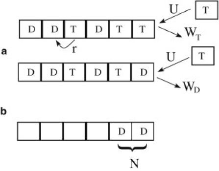
(a) Representation of the various elementary transitions considered in the model with their corresponding rates, U the on-rate of GTP-subunits, WT the off-rate of GTP-subunits, WD the off-rate of GDP-subunits, and r the hydrolysis rate for each unhydrolyzed unit within the filament. (b) Pattern for a catastrophe with N terminal units in the GDP state.
Table 1.
Various rates used in the model and corresponding references
| Description | Symbols | Rates for Figs. 1–3a, and Figs. 4–8 | Rates for Fig. 3b | References |
|---|---|---|---|---|
| On-rate of T subunits (plus-end) | K0 (μM−1 s−1) | 3.2 | 3.2 | Howard (33) |
| Off-rate of T subunits (plus-end) | WT (s−1) | 24 | 0 | Janson et al. (21); Rate for Fig. 3b is from Drechsel et al. (34) |
| Off-rate of D subunits (plus-end) | WD (s−1) | 290 | 290 | Howard (33) |
| Hydrolysis rate (random model) | r (s−1) | 0.2 | 0.25 |
Conditions are that of a low ionic strength buffer. The value used for the rate of hydrolysis results from the analysis of this article.
As a result of the random hydrolysis, a typical filament configuration contains many islands of unhydrolyzed subunits within the filament. The last island containing the terminal unit is called the “cap”.
Results and Discussion
Nucleotide content of the filament
In this section, we obtain the nucleotide content of the filament within a mean-field approximation (for earlier references on this model, see Stukalin and Kolomeisky (11), Ranjith et al. (15), and Keiser et al. (35)). We denote by i the position of a monomer within the filament, from the terminal unit at i = 1. For a given configuration, we introduce for each subunit i an occupation number τi, such that τi = 1 if the subunit is bound to GTP and τi = 0 otherwise. In the reference frame associated with the end of the filament, the equations for the average occupation number are for i = 1,
| (1) |
and for i > 1,
| (2) |
In a mean-field approach, correlations are neglected, which means that for any i, j, 〈τi τj〉 is replaced by 〈τi〉〈τj〉. At steady state, the left-hand sides of Eqs. 1 and 2 are both zero, which leads to recursion relations for the 〈τi〉. Let us denote 〈τi〉 = q as the probability that the terminal unit is bound to GTP. The recursion relations have a solution of the form for i ≥ 1,
| (3) |
where
Combining Eqs. 1–3, one obtains q explicitly as function of all the rates as the solution of a cubic equation that is given in the Appendix of Ranjith et al. (15). The mean filament velocity (namely the average rate of change of the total filament length) is given by
| (4) |
in terms of the monomer size d. More precisely, in our model d = 8 nm/13 = 0.6 nm, corresponding to the length of a tubulin monomer divided by 13, which is the average number of protofilaments in a microtubule. At the critical concentration cc, the mean velocity vanishes, which corresponds to the boundary between a phase of bounded growth for c < cc and a phase of unbounded growth for c > cc (15). The plot of this velocity versus concentration exhibits a kink shape near the critical concentration, which is not particularly sensitive to the mechanism of hydrolysis because it is present both in the vectorial and random model (11,15). This kink is well known from studies with actin (36) but has not been studied experimentally with microtubules except in Carlier et al. (28) in a specific medium containing glycerol.
The distribution of the nucleotide along the filament length has a well-defined steady state in the tip reference frame at arbitrary value of the monomer concentration c. Using Eq. 3, it follows that 〈τi〉 = bi−1q, and therefore, the steady-state probability that the cap has exactly a length l, Pl, is
This leads to the expression
| (5) |
and the corresponding average cap size is
In Fig. 2, we show how this average cap size varies as function of the free tubulin concentration. The average cap becomes longer than approximatively one subunit above the critical concentration, cc defined above, and which is ∼7 μM for the parameters of Table 1 used here. At concentrations significantly larger than this value, the cap's average size increases more slowly, as as U → ∞ (9,13). In the range of concentration [0:100 μM], the cap stays smaller than ∼47 subunits, which represents only 3.6 layers (or 28 nm). This estimate indicates that the cap is below optical resolution in the range of tubulin concentration generally used, which could explain the difficulty for observing it experimentally.
Figure 2.
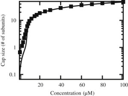
Average cap size in number of subunits as function of the free tubulin concentration c in μM. The line is the mean-field analytical solution and (solid squares) are simulation points.
A long-standing view in the literature is that the cap could be as small as a single layer, as shown by experiments based on a chemical detection of the phosphate release (37). This view has been recently challenged by two experiments, in which the length fluctuations of microtubules were probed at the nanoscale (25,26). The interpretation of these experiments still generates debates (38,39); however, in any case, taken together these studies reported a highly variable MT plus-end growth behavior, which suggests that the cap size is a fluctuating quantity, larger than one layer but smaller than ∼5 layers. We note that such a range is compatible with our prediction and agrees with the estimation obtained from dilution experiments (23). Furthermore, our stochastic model naturally incorporates a fluctuating cap size. Even if the cap is indeed below optical resolution, we note that this does not rule out the possibility that it could be observed with the technique of Dimitrov et al. (24).
In Fig. 2, we also compare the predictions of the mean-field approximation with an exact simulation of the dynamics. We find that mean-field theory provides an excellent approximation of the exact solution when the free tubulin concentration is above the critical concentration, which corresponds to the conditions of most experiments (21,22). Deviations can be seen between the exact solution and its mean-field approximation in Fig. 2 but only below the critical concentration. Many other quantities of interest follow from the determination of the nucleotide content of a given subunit, namely 〈τi〉, such as the length fluctuations of the filament (15) or the islands distribution of hydrolyzed or nonhydrolyzed subunits (13,17). These predictions should prove particularly useful in testing this model against experiments, because the island distribution of unhydrolyzed units or remnants may become accessible in future experiments similar to that of Dimitrov et al. (24), but carried out in in vitro conditions.
Frequency of catastrophes and rescues versus concentration
One difficulty in bridging the gap between a model of the dynamic instability and experiments lies in a proper definition of the event that is called a catastrophe, because the number of reported catastrophes is affected by several factors depending on the experimental conditions, such as, for instance, the experimental resolution of the observation (25).
Although a catastrophe manifests itself experimentally as an abrupt reduction of the total filament length, we choose to define it from the nucleotide content of the terminal region. Following closely Brun et al. (29), we define a shrinking configuration as one in which the last N units of the filament are all in the GDP state (irrespective of the state of the other units) as shown in Fig. 1. The remaining configurations (with an unhydrolyzed cap of any size or when the number of hydrolyzed subunits at the end is <N) are assumed to belong to the growing phase. We emphasize that this means that transitions to a shrinking configuration (i.e., catastrophes) occur without the filament having been necessarily peeled off to its end. This is an important difference with the model mentioned above (29), which did not include rescues. Our approach can include rescues and takes into account the finite rate of loss of GDP units. Another difference is that the model of Brun et al. (29) corresponds to the regime of high concentration of free subunits, whereas our model holds at any concentration—even in the proximity or below the critical concentration.
To understand the physical meaning of the parameter N, an analogy with nucleation theory can be helpful. In our model, N plays the role of the critical nucleus in nucleation theory, because we are interested here in the “nucleation” of a catastrophe rather than the nucleation of a filament.
Within the two-state description of the dynamics (with a growing and a shrinking phase) outlined above and implicitly assumed in the analysis of most experiments, the catastrophe frequency fc(N) is the inverse of the average time spent in the growing phase, whereas the rescue frequency fr(N) is the inverse of the average time spent in the shrinking phase. It follows that the catastrophe frequency fc(N) can be obtained as the probability flux out of the growing state divided by the probability to be in the growing state. For instance for N = 1, this flux condition is
| (6) |
where the terms on the right proportional to P1 correspond to a transition of the terminal unit from the GTP to the GDP state, which can occur either through hydrolysis or depolymerization of that unit, while the last term corresponds to hydrolysis of the terminal unit from cap states of length ≥ 2. We have derived the general expression of fc(N) in the case of an arbitrary N as shown in the Supporting Material, and we have checked these results by comparing them with stochastic simulations using the Gillespie algorithm (40).
In the case of the vectorial model, the last term in Eq. 6 is absent and the catastrophe frequency is nonzero only below the critical concentration. The fact that catastrophes are observed in Janson et al. (21) significantly above the critical concentration indicates that this data are incompatible with a vectorial mechanism. For this reason, we only discuss here the predictions of the random model.
The time between catastrophes, Tc(N) = 1/fc(N) is shown as function of growth velocity for N = 2 and compared to the experimental data of Janson et al. (21) in Fig. 3 a and to the experimental data of Drechsel et al. (34) in Fig. 3 b. Note that each figure corresponds to a different choice for the value of the parameter WT as explained in Table 1. In both cases, we have observed that the experimental data can be well fitted with our model provided we take N = 2 but not N = 1. The same observation has been made in Brun et al. (29), where the experimental data (21) have also been analyzed. We can propose an explanation based on the analogy mentioned above with nucleation theory. In classical nucleation theory, it is not possible to consider a critical nucleus size equal to a monomer, similarly here the case N = 1 does not make physical sense. From the same argument, it follows that it is also not very meaningful to consider catastrophes defined from a high value of N, because a critical nucleus has to be minimal. Thus the analogy explains why the choice N = 2 is the most pertinent one to analyze experiments.
Figure 3.
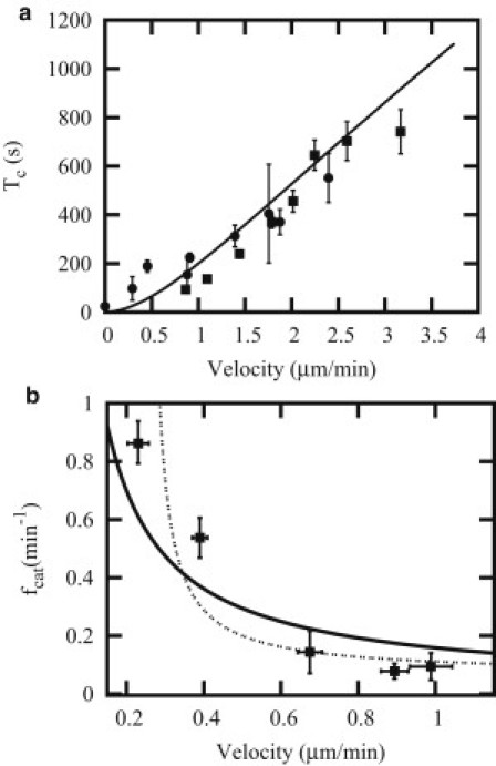
(a) Catastrophe time Tc versus growth velocity for the N = 2 case, with the theoretical prediction (solid line) together with simulation points (solid squares) and experimental data points taken from Janson et al. (21) for constrained growth and free growth (solid circles). (Error bars) Simulation points have been obtained using the block-averaging method (41). (b) Catastrophe frequency (fcat = 1/Tc) versus velocity: our mean-field theory result (continuous curve) is compared with experiments of Drechsel et al. (34) (solid squares with error bars) and theory of Flyvbjerg et al. (9) (dotted curve).
In Fig. 3 b, we have shown the prediction from our model together with that from Flyvbjerg et al. (9). This comparison shows that the prediction deduced from this reference has a sharp increase around a value of growth velocity of 0.3 μm/min, which is not clearly present in the experimental data and in our model. Furthermore, the value obtained for the hydrolysis rate is similar between the two experiments of Fig. 3, a and b, in both cases r ≂ 0.3 s−1. This value is also close to the estimate r ≂ 0.3 s−1 obtained in Piette et al. (27) through a fit of dilution experiments, discussed in the next section.
We also show the distribution of catastrophe times calculated with the parameters given in Table 1, for N = 2 in Fig. 4. These distributions are nonexponential, but the peak in the distribution occurs at a very small time, so that, in practice, in the conditions of the observations of Janson et al. (21) with free filaments, the distribution will appear exponential as found experimentally.
Figure 4.
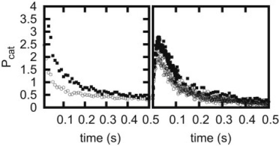
(Left) Distribution of catastrophe time (N = 1) for different concentration values. C = 9 μM (solid squares) and C = 12 μM (open circles). (Right) The distribution of catastrophe time (N = 2) for different concentration values C = 9 μM (solid squares) and C = 12 μM (open circles). The distributions are normalized such that area under the curve is 1.
Another advantage of our model is that it can explain other aspects of the dynamic instability of microtubules that were not considered in previous models such as those of Flyvbjerg et al. (9) and Brun et al. (29). Specifically, it also allows us to predict the statistics of rescue events when the polymer switches from the shrinking phase back into the growing phase. Assuming that the system reached a steady-state behavior, the frequency of rescues fr(N) can be calculated using flux conditions similar to the ones used to obtain fc(N) (see the Supporting Material for more details). The corresponding expression is rather simple and it can be written as
| (7) |
We have carried out a complete numerical test of this expression of the frequency of rescues using stochastic simulations, which is shown later in Fig. 8. In the conditions of this figure, the filaments are sufficiently long and thus they do not collapse before rescue events occur. The theoretical mean-field predictions agree well with the simulations at concentrations of free monomers larger than the critical concentration. Deviations are observed at low concentrations near the critical concentration, in a way that has similarities with the deviations observed in Fig. 2.
Figure 8.
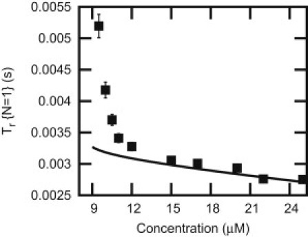
Rescue time (N = 1) as function of concentration. (Solid line) Obtained from the mean-field theory. Data points (solid squares) are obtained from the simulations.
Our model predicts that rescues should be observable under typical cellular conditions and in experiments. However, surprisingly there is a very limited experimental information on rescues. The analysis of Eq. 7 might shed some light on this issue. At low concentrations of GTP monomers in the solution, when the rate U is small, the average time before the rescue event, Tr ≃ 1/U, might be very large. As a result, it might not be observable in experiments because the polymer with L monomers could depolymerize faster (Tcollapse ≃ L/WD) before any rescue event could take place. At large U, rescues are more frequent given that the polymer is in the shrinking state. However, frequency of the catastrophes is very small under these conditions, and the microtubule is almost always in the growing phase. Therefore, in these conditions, rescues are not observed (21).
First passage time of the cap and dilution experiments
The first passage time of the cap is a key quantity to understand the statistics of catastrophes and the dilution experiments. Let us define Fk(t) as the distribution of the first passage time Tk for an initial condition corresponding to a cap of length k, and a filament in contact with a medium of arbitrary concentration. As shown in Appendix, one can calculate analytically Fk(t), by a method recently used in the context of polymer translocation (42). After numerically inverting the Laplace transform of Fk(t), one obtains the distribution Fk(t), which is shown as solid lines in Fig. 5 for the particular case of k = 2. As can be seen in this figure, the predicted distributions agree very well with the results obtained from the stochastic simulation in this case.
Figure 5.
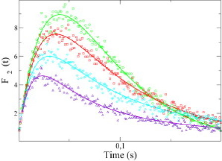
Distributions of the first passage time of the cap for an initial cap of k = 2 units, F2(t) as function of the time t, for various initial concentration of free monomers. (Solid lines) Theoretical predictions deduced from Eq. 16 of the Appendix after numerically inverting the Laplace transform. (Symbols) Simulations. (Circles) Dilution into a medium with no free monomers; (squares) dilution into a medium with a concentration of free monomers of 2 μM; (diamonds) 5 μM; and (triangles) 9 μM.
From the distribution Fk(t) we obtain its first moment, the mean first-passage time of the cap 〈T(k)〉. We find that
| (8) |
where
and the functions Jn(y) are Bessel functions. The dependence of 〈T(k)〉 as a function of the initial size of the cap k is shown in Fig. 6: at small k, 〈T(k)〉 is essentially linear in k as would be expected at all k in the vectorial model of hydrolysis (14), whereas here it saturates at large values of k (the value of this plateau can be calculated analytically but only for U = 0, see Appendix). To understand this saturation, consider a cap that is initially infinitively large, then after a time of order 1/r, the cap abruptly becomes of a finite much smaller size as a result of the hydrolysis of one unit at a random position within the filament. This feature will always happen irrespective of the monomer concentration, and indeed in Fig. 6, 〈T(k)〉 has a plateau for k → ∞ for all values of the monomer concentration. We note that such a behavior of 〈T(k)〉 as function of k has similarities with the case of noncompact exploration investigated in Condamin et al. (43), whereas the vectorial model of hydrolysis would correspond in the language of this reference to the case of compact exploration.
Figure 6.
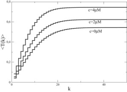
Mean first-passage time 〈T(k)〉 as function of k for three values of the monomer concentration from bottom to top 0, 2, and 4 μM. The presence of steps in these curves is due to the fact that 〈T(k)〉 is only defined on integer values of k. Note the existence of a plateau for all values of the monomer concentration.
Let us now turn to a practical use of this quantity for understanding dilution experiments. In these experiments, the concentration of free tubulin is abruptly reduced to a small value, resulting in catastrophes within seconds, independent of the initial concentration (23,44). This observation is an evidence that the cap is short and independent of the initial concentration. The idea that the cap is short is also supported by the observation that cutting the end of a microtubule typically with a laser results in catastrophe. As we shall see below, all these well-known experimental facts about microtubules can be explained by our model.
For simplicity, we illustrate the method with the definition of catastrophe introduced in the previous section for N = 1, which means that a catastrophe starts as soon as the cap has disappeared. As shown in the previous section, the method could be extended to the more general case of an arbitrary N. The characteristic time observed in dilution experiments, Tdilution, is a special average over 〈T(k)〉. More precisely, let us denote 〈T(k)〉post as the first passage time in postdilution conditions given that the initial length of the cap is k. The delay time before catastrophe Tdilution is then the average of 〈T(k)〉post with respect to the steady-state probability distribution of the initial conditions before the dilution occurs. In other words,
| (9) |
where Pk(predilution) is the stationary probability given in Eq. 5 in predilution conditions.
In the case that the final medium after dilution is very dilute, one can assume that the final free tubulin concentration is zero, which allows us to simplify significantly Eq. 8 as explained in the Appendix. Using Eq. 9, one obtains the delay time before first catastrophe for the parameters of the Table 1 that is shown in Fig. 7. The figure confirms that the delay time can be as short as a fraction of seconds in this case. It is straightforward to extend this calculation to the case of an arbitrary value of the postdilution medium (i.e., for the case of a dilution of arbitrary strength) using Eq. 8. As the amplitude of the dilution is reduced (by increasing the postdilution concentration), the delay time increases as well but the general sigmoidal shape remains, with in particular a plateau at concentrations above the critical concentration. The presence of these plateaux means that the delay time is essentially independent of the concentration of the monomers in predilution conditions as observed experimentally. It is satisfying to see that the determination of the hydrolysis rate from the catastrophe frequencies is close to the value obtained through a fit of dilution experiments as done in Piette et al. (27). Thus, complementary and consistent information can be obtained from the statistics of catastrophes and from dilution times.
Figure 7.
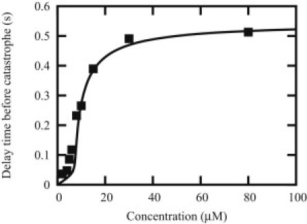
Delay time before catastrophe (s) as function of free tubulin concentration (in μM) before dilution in the case that the postdilution tubulin concentration is zero. (Solid line) Mean-field prediction based on Eq. 9; (symbols) simulation points. As found experimentally, the delay time is essentially independent of the concentration of tubulin in the predilution state, and the time to observe the first catastrophe is of the order of seconds or less.
Conclusion
In this work, we have constructed a model of microtubule dynamics that only includes the random spontaneous phosphate release within the filament. Despite its simplicity in the description of the hydrolysis process, the model is very rich and can account for many aspects of microtubule dynamics, such as the mean catastrophe time and its distribution or the delays after a dilution. We have also investigated much less studied aspects concerning the cap size, the role of the definition of catastrophes (via the parameter N), the first passage time of the cap, and the statistics of rescues.
The theoretical model and ideas presented in this article for microtubules could also apply to other biofilaments such as actin or Par-M, for which the random hydrolysis model may be relevant as well. In fact, a very recent experimental study (20) confirmed the pertinence of random hydrolysis for actin. Furthermore, the model could be extended to include the dynamics of the minus-end as in Ranjith et al. (15), or to investigate, for instance, the unexpected stability of the minus-end reported in (45).
Finally, although the model describes a priori only single free filaments dynamics, it is also potentially useful for understanding constrained filaments, in the broader context of force generation and force regulation by ensembles of biofilaments. For this reason, it would be interesting to study extensions of the model to account for the various effects of microtubule-associated proteins on microtubules, which should shed light on the behavior of microtubules in more realistic biological conditions. We hope that this theoretical work will stimulate further experimental and theoretical studies of these questions.
While our paper was under review, we came across a new work by Gardner et al. (46), which provides new, interesting insights into the dynamics of single microtubule filament.
Acknowledgments
We thank F. Perez, F. Nedelec, and M. F. Carlier for inspiring discussions. We also thank K. Mallick for pointing us to Krapivsky and Mallick (42), and M. Dogterom for providing us with the data of Janson et al. (21).
R.P. acknowledges support from the Department of Biotechnology India through the Innovative Young Biotechnologist Award. A.B.K. acknowledges support from the Welch Foundation (grant No. C-1559) and from the U.S. National Science Foundation (grant No. ECCS-0708765). D.L. acknowledges support from the French National Research Agency under contract No. ANR-09-PIRI-0001-02.
Contributor Information
Ranjith Padinhateeri, Email: ranjithp@iitb.ac.in.
Anatoly B. Kolomeisky, Email: tolya@rice.edu.
David Lacoste, Email: david@turner.pct.espci.fr.
Appendix: A Distribution of First Passage Time of the Cap in the Random Model
Let us denote by Fk(t) the probability distribution of the first passage time of the GTP-tip (also called “cap” in the main text), for a cap that is initially of length k. This quantity obeys the following backward master equation, for ,
| (10) |
These equations are supplemented by the boundary condition F0(t) = δ(t). We will assume that the random walk followed by the cap is recurrent, which means here that the disappearance of the cap is certain, whatever the time it takes. That condition means that for all k ≥ 0,
We will make use of the Laplace transform of Fk(t) defined by
With this definition, the equations above take the following form, again for k ≥ 1,
| (11) |
with the conditions and for all k ≥ 0, , which follows from the normalization condition and the definition of the Laplace transform above.
For the applications of this first passage time distribution to dilution experiments, we are interested mainly in calculating it using postdilution conditions. In the case of a dilution, the concentration of the free monomers after dilution is, in general, small. Let us discuss separately the particular case where the concentration of the medium after dilution is zero in which case U = 0, and the general case of a dilution into a medium of prescribed concentration corresponding to U ≠ 0.
Particular case of U = 0
In this particular case, the recursion equations given in Eq. 11 are easy to solve. The solution is
| (12) |
for k ≥ 1, with the convention that a sum over an index that ends at 0 is void. The mean first-passage time T(k), is the first moment of Fk(t), and thus satisfies
It follows that for k ≥ 1,
| (13) |
In this particular case of U = 0, it is possible to derive an asymptotic form of this mean first-passage time for k → ∞, namely 〈T〉 = limk→∞ 〈T(k)〉. Indeed in this case, the sum can be written in terms of hypergeometric functions (13,47), and it reads
The expression of the mean first-passage time given in Eq. 13 can be used to obtain the delay before the appearance of the first catastrophe, as explained in the main text. In this case, we find
where
This dilution time is shown in Fig. 7 of the main text.
General case of U ≠ 0
The solution to this general case is more involved but it can be obtained using Bessel functions (for a solution of a similar recursion, see Krapivsky and Mallick (42)). In a first step, we transform the recursion of Eq. 11 using the difference variable , which leads to
| (14) |
Then, we introduce the change of variable Kk(s) = ykgk(s), and we choose in such a way that Eq. 14 takes the simpler form
| (15) |
The solution to this equation can be obtained by comparing with the well-known identity
for Bessel functions. Thus, the solution has the form
| (16) |
where C is a constant and . The boundary condition given above for leads to the following condition that fixes the constant C. In the end, one obtains
| (17) |
which satisfies, in addition, the required condition at s = 0, namely that for all k ≥ 0, gk(s = 0) = 0. With this expression, one obtains the Laplace transform of the first passage distribution of the cap, , from
| (18) |
Although it is not immediately apparent, it can be checked that the particular case discussed above is indeed recovered by taking the limit U → 0 of the general case. After using together with Eq. 18, one obtains the general expression for the mean first-passage time of the cap 〈T(k)〉 given in the main text, which reads
| (19) |
where .
Supporting Material
References
- 1.Desai A., Mitchison T.J. Microtubule polymerization dynamics. Annu. Rev. Cell Dev. Biol. 1997;13:83–117. doi: 10.1146/annurev.cellbio.13.1.83. [DOI] [PubMed] [Google Scholar]
- 2.Margolis R.L., Wilson L. Microtubule treadmilling: what goes around comes around. Bioessays. 1998;20:830–836. doi: 10.1002/(SICI)1521-1878(199810)20:10<830::AID-BIES8>3.0.CO;2-N. [DOI] [PubMed] [Google Scholar]
- 3.Mitchison T., Kirschner M. Dynamic instability of microtubule growth. Nature. 1984;312:237–242. doi: 10.1038/312237a0. [DOI] [PubMed] [Google Scholar]
- 4.Bayley P.M., Schilstra M.J., Martin S.R. A simple formulation of microtubule dynamics: quantitative implications of the dynamic instability of microtubule populations in vivo and in vitro. J. Cell Sci. 1989;93:241–254. doi: 10.1242/jcs.93.2.241. [DOI] [PubMed] [Google Scholar]
- 5.Hill T.L. Introductory analysis of the GTP-cap phase-change kinetics at the end of a microtubule. Proc. Natl. Acad. Sci. USA. 1984;81:6728–6732. doi: 10.1073/pnas.81.21.6728. [DOI] [PMC free article] [PubMed] [Google Scholar]
- 6.Dogterom M., Leibler S. Physical aspects of the growth and regulation of microtubule structures. Phys. Rev. Lett. 1993;70:1347–1350. doi: 10.1103/PhysRevLett.70.1347. [DOI] [PubMed] [Google Scholar]
- 7.Verde F., Dogterom M., Leibler S. Control of microtubule dynamics and length by cyclin A- and cyclin B-dependent kinases in Xenopus egg extracts. J. Cell Biol. 1992;118:1097–1108. doi: 10.1083/jcb.118.5.1097. [DOI] [PMC free article] [PubMed] [Google Scholar]
- 8.Flyvbjerg H., Holy T.E., Leibler S. Stochastic dynamics of microtubules: a model for caps and catastrophes. Phys. Rev. Lett. 1994;73:2372–2375. doi: 10.1103/PhysRevLett.73.2372. [DOI] [PubMed] [Google Scholar]
- 9.Flyvbjerg H., Holy T.E., Leibler S. Microtubule dynamics: caps, catastrophes, and coupled hydrolysis. Phys. Rev. E. 1996;54:5538–5560. doi: 10.1103/physreve.54.5538. [DOI] [PubMed] [Google Scholar]
- 10.Margolin G., Gregoretti I.V., Alber M.S. Analysis of a mesoscopic stochastic model of microtubule dynamic instability. Phys. Rev. E. 2006;74:041920. doi: 10.1103/PhysRevE.74.041920. [DOI] [PubMed] [Google Scholar]
- 11.Stukalin E.B., Kolomeisky A.B. ATP hydrolysis stimulates large length fluctuations in single actin filaments. Biophys. J. 2006;90:2673–2685. doi: 10.1529/biophysj.105.074211. [DOI] [PMC free article] [PubMed] [Google Scholar]
- 12.Zong C., Lu T., Wolynes P.G. Nonequilibrium self-assembly of linear fibers: microscopic treatment of growth, decay, catastrophe and rescue. Phys. Biol. 2006;3:83–92. doi: 10.1088/1478-3975/3/1/009. [DOI] [PubMed] [Google Scholar]
- 13.Antal T., Krapivsky P.L., Chakraborty B. Dynamics of an idealized model of microtubule growth and catastrophe. Phys. Rev. E. 2007;76:041907. doi: 10.1103/PhysRevE.76.041907. [DOI] [PMC free article] [PubMed] [Google Scholar]
- 14.Ranjith P., Lacoste D., Joanny J.F. Nonequilibrium self-assembly of a filament coupled to ATP/GTP hydrolysis. Biophys. J. 2009;96:2146–2159. doi: 10.1016/j.bpj.2008.12.3920. [DOI] [PMC free article] [PubMed] [Google Scholar]
- 15.Ranjith P., Mallick K., Lacoste D. Role of ATP-hydrolysis in the dynamics of a single actin filament. Biophys. J. 2010;98:1418–1427. doi: 10.1016/j.bpj.2009.12.4306. [DOI] [PMC free article] [PubMed] [Google Scholar]
- 16.Pieper U., Wegner A. The end of a polymerizing actin filament contains numerous ATP-subunit segments that are disconnected by ADP-subunits resulting from ATP hydrolysis. Biochemistry. 1996;35:4396–4402. doi: 10.1021/bi9527045. [DOI] [PubMed] [Google Scholar]
- 17.Li X., Lipowsky R., Kierfeld J. Coupling of actin hydrolysis and polymerization: reduced description with two nucleotide states. Europhys. Lett. 2010;89:38010. [Google Scholar]
- 18.Kueh H.Y., Mitchison T.J. Structural plasticity in actin and tubulin polymer dynamics. Science. 2009;325:960–963. doi: 10.1126/science.1168823. [DOI] [PMC free article] [PubMed] [Google Scholar]
- 19.Valiron O., Arnal I., Job D. GDP-tubulin incorporation into growing microtubules modulates polymer stability. J. Biol. Chem. 2010;285:17507–17513. doi: 10.1074/jbc.M109.099515. [DOI] [PMC free article] [PubMed] [Google Scholar]
- 20.Jégou A., Niedermayer T., Romet-Lemonne G. Individual actin filaments in a microfluidic flow reveal the mechanism of ATP hydrolysis and give insight into the properties of profilin. PLoS Biol. 2011;9:e1001161. doi: 10.1371/journal.pbio.1001161. [DOI] [PMC free article] [PubMed] [Google Scholar]
- 21.Janson M.E., de Dood M.E., Dogterom M. Dynamic instability of microtubules is regulated by force. J. Cell Biol. 2003;161:1029–1034. doi: 10.1083/jcb.200301147. [DOI] [PMC free article] [PubMed] [Google Scholar]
- 22.Walker R.A., O'Brien E.T., Salmon E.D. Dynamic instability of individual microtubules analyzed by video light microscopy: rate constants and transition frequencies. J. Cell Biol. 1988;107:1437–1448. doi: 10.1083/jcb.107.4.1437. [DOI] [PMC free article] [PubMed] [Google Scholar]
- 23.Voter W.A., O'Brien E.T., Erickson H.P. Dilution-induced disassembly of microtubules: relation to dynamic instability and the GTP cap. Cell Motil. Cytoskeleton. 1991;18:55–62. doi: 10.1002/cm.970180106. [DOI] [PubMed] [Google Scholar]
- 24.Dimitrov A., Quesnoit M., Perez F. Detection of GTP-tubulin conformation in vivo reveals a role for GTP remnants in microtubule rescues. Science. 2008;322:1353–1356. doi: 10.1126/science.1165401. [DOI] [PubMed] [Google Scholar]
- 25.Schek H.T., 3rd, Gardner M.K., Hunt A.J. Microtubule assembly dynamics at the nanoscale. Curr. Biol. 2007;17:1445–1455. doi: 10.1016/j.cub.2007.07.011. [DOI] [PMC free article] [PubMed] [Google Scholar]
- 26.Kerssemakers J.W.J., Munteanu E.L., Dogterom M. Assembly dynamics of microtubules at molecular resolution. Nature. 2006;442:709–712. doi: 10.1038/nature04928. [DOI] [PubMed] [Google Scholar]
- 27.Piette B.M.A.G., Liu J., Hussey P.J. A thermodynamic model of microtubule assembly and disassembly. PLoS ONE. 2009;4:e6378. doi: 10.1371/journal.pone.0006378. [DOI] [PMC free article] [PubMed] [Google Scholar]
- 28.Carlier M.F., Hill T.L., Chen Y. Interference of GTP hydrolysis in the mechanism of microtubule assembly: an experimental study. Proc. Natl. Acad. Sci. USA. 1984;81:771–775. doi: 10.1073/pnas.81.3.771. [DOI] [PMC free article] [PubMed] [Google Scholar]
- 29.Brun L., Rupp B., Nédélec F. A theory of microtubule catastrophes and their regulation. Proc. Natl. Acad. Sci. USA. 2009;106:21173–21178. doi: 10.1073/pnas.0910774106. [DOI] [PMC free article] [PubMed] [Google Scholar]
- 30.Jánosi I.M., Chrétien D., Flyvbjerg H. Structural microtubule cap: stability, catastrophe, rescue, and third state. Biophys. J. 2002;83:1317–1330. doi: 10.1016/S0006-3495(02)73902-7. [DOI] [PMC free article] [PubMed] [Google Scholar]
- 31.VanBuren V., Cassimeris L., Odde D.J. Mechanochemical model of microtubule structure and self-assembly kinetics. Biophys. J. 2005;89:2911–2926. doi: 10.1529/biophysj.105.060913. [DOI] [PMC free article] [PubMed] [Google Scholar]
- 32.Mohrbach H., Johner A., Kulić I.M. Tubulin bistability and polymorphic dynamics of microtubules. Phys. Rev. Lett. 2010;105:268102. doi: 10.1103/PhysRevLett.105.268102. [DOI] [PubMed] [Google Scholar]
- 33.Howard J. Sinauer Associates; Sunderland, MA: 2001. Mechanics of Motor Proteins and the Cytoskeleton. [Google Scholar]
- 34.Drechsel D.N., Hyman A.A., Kirschner M.W. Modulation of the dynamic instability of tubulin assembly by the microtubule-associated protein tau. Mol. Biol. Cell. 1992;3:1141–1154. doi: 10.1091/mbc.3.10.1141. [DOI] [PMC free article] [PubMed] [Google Scholar]
- 35.Keiser T., Schiller A., Wegner A. Nonlinear increase of elongation rate of actin filaments with actin monomer concentration. Biochemistry. 1986;25:4899–4906. doi: 10.1021/bi00365a026. [DOI] [PubMed] [Google Scholar]
- 36.Pantaloni D., Hill T.L., Korn E.D. A model for actin polymerization and the kinetic effects of ATP hydrolysis. Proc. Natl. Acad. Sci. USA. 1985;82:7207–7211. doi: 10.1073/pnas.82.21.7207. [DOI] [PMC free article] [PubMed] [Google Scholar]
- 37.Panda D., Miller H.P., Wilson L. Determination of the size and chemical nature of the stabilizing “cap” at microtubule ends using modulators of polymerization dynamics. Biochemistry. 2002;41:1609–1617. doi: 10.1021/bi011767m. [DOI] [PubMed] [Google Scholar]
- 38.Howard J., Hyman A.A. Growth, fluctuation and switching at microtubule plus ends. Nat. Rev. Mol. Cell Biol. 2009;10:569–574. doi: 10.1038/nrm2713. [DOI] [PubMed] [Google Scholar]
- 39.Gardner M.K., Hunt A.J., Odde D.J. Microtubule assembly dynamics: new insights at the nanoscale. Curr. Opin. Cell Biol. 2008;20:64–70. doi: 10.1016/j.ceb.2007.12.003. [DOI] [PMC free article] [PubMed] [Google Scholar]
- 40.Gillespie D.T. Exact stochastic simulation of coupled chemical reactions. J. Phys. Chem. 1977;81:2340. [Google Scholar]
- 41.Frenkel D., Smit D. Academic Press; New York: 2002. Understanding Molecular Simulations. [Google Scholar]
- 42.Krapivsky P.L., Mallick K. Fluctuations in polymer translocation. J. Stat. Mech. 2010;2010:P07007. [Google Scholar]
- 43.Condamin S., Bénichou O., Klafter J. First-passage times in complex scale-invariant media. Nature. 2007;450:77–80. doi: 10.1038/nature06201. [DOI] [PubMed] [Google Scholar]
- 44.Walker R.A., Pryer N.K., Salmon E.D. Dilution of individual microtubules observed in real time in vitro: evidence that cap size is small and independent of elongation rate. J. Cell Biol. 1991;114:73–81. doi: 10.1083/jcb.114.1.73. [DOI] [PMC free article] [PubMed] [Google Scholar]
- 45.Tran P.T., Walker R.A., Salmon E.D. A metastable intermediate state of microtubule dynamic instability that differs significantly between plus and minus ends. J. Cell Biol. 1997;138:105–117. doi: 10.1083/jcb.138.1.105. [DOI] [PMC free article] [PubMed] [Google Scholar]
- 46.Gardner M.K., Charlebois B.D., Odde D.J. Rapid microtubule self-assembly kinetics. Cell. 2011;146:582–592. doi: 10.1016/j.cell.2011.06.053. [DOI] [PMC free article] [PubMed] [Google Scholar]
- 47.Abramamowitz M., Stegun I.A. Dover; Mineola, New York: 1972. Handbook of Mathematical Functions. [Google Scholar]
Associated Data
This section collects any data citations, data availability statements, or supplementary materials included in this article.