A Bayesian approach to targeted experiment design

Abstract

Motivation: Systems biology employs mathematical modelling to further our understanding of biochemical pathways. Since the amount of experimental data on which the models are parameterized is often limited, these models exhibit large uncertainty in both parameters and predictions. Statistical methods can be used to select experiments that will reduce such uncertainty in an optimal manner. However, existing methods for optimal experiment design (OED) rely on assumptions that are inappropriate when data are scarce considering model complexity.

Results: We have developed a novel method to perform OED for models that cope with large parameter uncertainty. We employ a Bayesian approach involving importance sampling of the posterior predictive distribution to predict the efficacy of a new measurement at reducing the uncertainty of a selected prediction. We demonstrate the method by applying it to a case where we show that specific combinations of experiments result in more precise predictions.

Availability and implementation: Source code is available at: http://bmi.bmt.tue.nl/sysbio/software/pua.html

Contact: j.vanlier@tue.nl; N.A.W.v.Riel@tue.nl

Supplementary information: Supplementary data are available at Bioinformatics online.

1 INTRODUCTION

Computational models can be used to predict (un)measured behaviour or system responses and formalize hypotheses in a testable manner. To be able to make predictions parameters are required. Despite the development of new quantitative experimental techniques, data are often relatively scarce. Consequently the modeller is faced with a situation where large regions of parameter space can describe the measured data to an acceptable degree (Brännmark et al., 2010; Calderhead and Girolami, 2011; Girolami and Calderhead, 2011; Hasenauer et al., 2010; Raue et al., 2009). This is not a problem when the predictions required for testing the hypothesis (which we shall refer to as predictions of interest) are well constrained (Cedersund and Roll, 2009; Gomez-Cabrero et al., 2011; Gutenkunst et al., 2007; Kreutz et al., 2011; Tiemann et al., 2011). When this is not the case more data will be required. Optimal experiment design (OED) methods can be used to determine which experiments would be most useful in order to perform statistical inference. Classical design criteria are often based on linearization around a best fit parameter set (Kreutz and Timmer, 2009) and pertain to effectively constraining the parameters (Faller et al., 2003; Rodriguez-Fernandez et al., 2006) or predictions (Casey et al., 2007). However, when data are scarce considering the model complexity or the model is strongly non-linear, such methods are not appropriate (Kreutz et al., 2011). This makes investigating the role of parameter uncertainty in OED a relevant topic to explore. We propose a method for experimental design that overcomes these issues by adopting a probabilistic approach which incorporates prediction uncertainty. Our method enables the modeller to target experimental efforts in order to selectively reduce the uncertainty of predictions of interest. Using our approach, multiple experiments can be designed simultaneously revealing potential benefits that might arise from specific combinations of experiments.

We focus on biochemical networks that can be modelled using a system of ordinary differential equations. These models comprise of equations which contain parameters (constant in time), inputs and state variables . Given a set of parameters, inputs and initial conditions these equations can subsequently be simulated. Measurements are performed on a subset and/or a combination of the total number of states in the model. Measurements are hampered by measurement noise while many techniques used in biology (e.g. western blotting) necessitate the use of scaling and offset parameters (Kreutz et al., 2007). We define as , which lists all the required variables to simulate the model.

(1)

(2)

(3)

In order to perform inference and experiment design an error model is required. For ease of notation we shall demonstrate our method using a Gaussian error model. If we consider M time series of length N₁, N₂,…, N_M hampered by such noise, we obtain Equation (4) for the probability density function of the output data. Here y^t is the true system with true parameters , where σ_i,j indicates the SD of a specific data point and K serves as a normalization constant.

(4)

(5)

Using Bayes' theorem, we obtain an expression for the posterior probability distribution over the parameters (Klinke, 2009). The posterior probability distribution is given by normalizing Equation (4) multiplied with the prior to a unit area. Here corresponds to the probability of observing dataset y given the true parameters . Both computational as well as methodological advances have made Markov Chain Monte Carlo (MCMC) an attractive option for obtaining samples from such a distribution (Geyer, 1992; Girolami and Calderhead, 2011; Klinke, 2009).

Given a sample of the posterior parameter distribution, predictions can be made by simulating the model for each of the parameter sets. The distribution of such predictions shall be referred to as the posterior predictive distribution (PPD) and reflects their uncertainty. Since all of these predictions are linked via the parameter distributions, the relations between the different predictions can be exploited for experimental design. By considering the effects of a new measurement on the PPD, it is possible to predict how useful an experiment would be. Our approach consists of a number of steps. First, we briefly mention how to compute the PPD. Subsequently we detail how to compute the efficacy of the new measurement. In a third step this measure is used for experimental design. We conclude by demonstrating the method by applying it to a case study.

2 APPROACH

In order to overcome the limitations of existing OED methods, a sampling-based approach for experimental design is proposed. This approach consists of four consecutive steps which we shall outline below.

2.1 Step 1. Computation of the posterior parameter distribution

The first step in the analysis is computing the posterior parameter distribution of the model based on the available data:

(6)

Here probability reflects a degree of belief and prior knowledge regarding the parameters is included in the form of priors, and denotes the conditional probability of the data given the model parameters. The unnormalized form of this function is often referred to as the likelihood function. Furthermore, refers to the prior distribution of the parameters.

In order to sample from the posterior distribution we employ a MCMC method known as the Metropolis–Hastings algorithm. This algorithm performs a random walk through parameter space where each subsequent step is based on a proposal distribution (centred on the current step) and an acceptance criterion based on the proposal and probability densities at the sampled points. In brief, after an initial burn-in period (which is discarded), MCMC methods generate samples from probability distributions whose probability densities are known up to a normalizing factor. The Metropolis–Hastings algorithm proceeds as follows:

1. Generate a sample by sampling from a proposal distribution based on the current state .

2. Compute the likelihood of the data and calculate , where refers to the prior density function.

3. Draw a random number γ from a uniform distribution between 0 and 1 and accept the new step if .

Here Q(θ₁→θ₂) refers to the proposal density from current parameter set θ₁ to θ₂. The ratio of Q ensures detailed balance, a sufficient condition for the Markov chain to converge to the equilibrium distribution (Neal, 1996). It corrects for sampling biases resulting from non-symmetric proposal distributions and is defined as the ratio between the proposal densities associated with going from n to n+1 and n+1 to n. We employ an adaptive Gaussian proposal distribution whose covariance matrix is based on a quadratic approximation to the posterior probability at the current sample point (Gutenkunst et al., 2007). Further details regarding the implementation can be found in the Supplementary Materials.

2.2 Step 2. Determine PPDs for all candidate experiments

A PPD is a distribution of predictions conditioned on the available data as shown in Equation (7). A PPD is obtained by simulating the model (including the addition of measurement noise) for a sample of parameter sets from the posterior parameter distribution. We simulate a PPD for each candidate experiment. These PPDs link the parameters to the predictions and via the parameters also link predictions (across different experiments) to each other. The model and data constrain the dynamics of the system and hereby implicitly impose non-trivial relations between the different predictions. Therefore, the observables of candidate experiments are related to our prediction of interest. The next step is to exploit the relations within these distributions for experimental design.

(7)

2.3 Step 3. Predict EVR based on PPDs and measurement accuracies

To be able to perform experiment design a measure of expected measurement efficacy is required. For this purpose, we introduce the expected variance reduction (EVR). Consider an independent new measurement of a specific prediction (observable). This new measurement is associated with an error model G which reflects a certain degree of uncertainty associated with the new experiment. If this new experiment were to be performed and a value is obtained, then the subsequent step would be to incorporate the new data point (and its associated error model) in the likelihood function and re-perform the MCMC. This new data would subsequently constrain the posterior parameter distribution, hence also affecting the prediction of interest (which cannot be measured directly). This process is illustrated in Figure 1.

Fig. 1.

Illustration of the effect of adding a new data point on the PPD. Shown on the top right is the PPD at one specific time point for two predictions with a subset of the samples of the chain indicated with white points. The square denotes the location of the ‘new measurement’. Prediction A refers to a prediction of which a new measurement can be performed (observable), whereas B denotes the prediction of interest. Here the grey distribution corresponds to the PPD before the new measurement, whereas the white Gaussian corresponds to the error model of the new measurement. Due to additional constraints imposed by this new measurement in combination with the old data and the model, the distribution on the hypothesis side is also updated in light of the new data point and shown in white.

The outcome of the experiment is known only after the experiment has been performed. Therefore the measured value in the error model is not known a priori. However, the PPD provides us with a predicted distribution of this value (shown in grey in Fig. 1) which reflects the uncertainty associated with this value. Samples from the PPD can subsequently be substituted as ‘true’ values in the error model. By repeating this process for every R-th point of our MCMC chain and averaging the result, we weight by the probability distribution of this predicted value. Considering that a single MCMC is often already computationally demanding, such a nested MCMC is likely not tractable. Here we propose an alternative approach. Consider the unnormalized densities , and , respectively, corresponding to the density model of the data used to determine the initial posterior distribution, the density model for the new data point, and the parameter prior. Assuming that the new data point is independent of the existing data points we can state that in order to obtain the following equation for the new normalized posterior (8). In this equation, Z₁ and Z₂ denote the normalization constants of the old and new posterior, respectively.

(8)

(9)

(10)

This relation between the two posteriors can be exploited in order to compute expected values by re-weighting samples from the old posterior appropriately. Rather than running a new MCMC for every sample, we can use self normalized importance sampling on the predictions of the output in order to compute expected values. This is shown in Equation (11), where samples and are taken from the old posterior distribution, T indicates the number of MCMC samples included in the analysis and indicates our quantity of interest.

(11)

As mentioned before, the value of y_n is not known a priori. Therefore, we subsequently compute such an expected value for each parameter set in the PPD with y_n set to the predicted output value from the original PPD. Hence this provides a distribution of expected values considering possible outcomes of the experiment. The mean of these expected values then provides us with a prediction of the quantity of interest. The entire approach can then be succinctly summarized in Equation (12). Here the expected value of z is computed, G corresponds to the error model and refers to the i-th parameter vector of the chain. Assuming a Gaussian error model with SD σ for a new measurement on the output y, probability model G is given by Equation (13). Note that both input as well as output can be any quantity of interest (prediction or parameter) indicating the flexibility of the approach.

(12)

(13)

Since the variance of a variable of interest can be computed by Equation (14), we can use the aforementioned method to estimate this quantity. The variance reduction can then be computed as shown in Equation (15) where σ_old² corresponds to the posterior variance without the new measurement and σ_new² corresponds to the expected posterior variance with the new measurements taken into account. In other words, one obtains the mean variance reduction considering the prediction uncertainty. The variance reduction computed by this sampling method is referred to as the sampled variance reduction (SVR).

(14)

(15)

2.3.1 Linear variance reduction:

When the measurement error models and PPD can reasonably be assumed Gaussian, one can approximate the variance reduction by approximating the PPD between the output and the measurements of interest with a multivariate Gaussian distribution. First the PD covariance matrix (16) is computed, where z denotes the output of interest and x^a_b the b-th MCMC sample of the a-th measurable state (without measurement noise), with Q and T the number of measured points and samples, respectively.

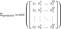(16)

After performing the new measurements with given SDs σ_b the covariance matrix is updated according to Equation (18). The resulting variance of the prediction of interest z can then be obtained as Σ_new(1, 1). We shall refer to the approximated variance reduction as the linear variance reduction (LVR).

(17)

(18)

2.4 Step 4. Determine measurement points for optimal variance reduction

The probability density model can be obtained by multiplying the error models for each candidate measurement. Subsequently, the space of all candidate measurements is sampled using Monte Carlo sampling. The efficacy of a specific combination of measurements is evaluated by computing the variance reduction, which is defined as Equation (15). During this sampling stage, additional constraints which arise because of practical considerations can be imposed on the experimental design (simply by rejecting such samples). An example of this could be the inability to measure certain states simultaneously. The optimal experiment is then obtained by determining the combination of measurements that yields the maximal predicted variance reduction.

3 COMPUTATIONAL METHODS

All of the discussed algorithms were implemented in Matlab (Natick, MA, USA). Numerical integration of the differential equations was performed with compiled MEX files using numerical integrators from the SUNDIALS CVode package (Lawrence Livermore National Laboratory, Livermore, CA, USA). Absolute and relative tolerances were set to 10⁻⁸ and 10⁻⁹, respectively. The Gaussian proposal distribution for the MCMC was based on an approximation to the Hessian computed using a Jacobian obtained using finite differencing (H≈J^TJ). All available priors were subsequently included in the Hessian approximation. After convergence, the chain was thinned to 10 000 samples. The SVR was computed in parallel using OpenCL on the GPU using a compiled MEX file.

4 RESULTS

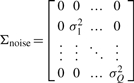
To illustrate our method, we apply it to a model of the JAK-STAT signalling pathway (Raue et al., 2009; Toni et al., 2009). The model is based on a number of hypothesized steps (See Figure 2). The first reaction describes the activation of the erythropoietin receptor which subsequently phosphorylates cytoplasmic STAT (x₁). Then phosphorylated STAT (x₂) dimerises (x₃) and is imported into the nucleus (x₄). Here dissociation and dephosphorylation occurs which are associated with a time delay. Similar to the implementation given in the original paper, the driving input function was approximated by a spline interpolant, while the delay was approximated using a linear chain approximation (x₅,…, x₁₃).

(19)

Fig. 2.

Model of the JAK-STAT pathway. In this model u₁ serves as driving input, while the total concentration of STAT (x₁+x₂+2x₃) and the total concentration of phosphorylated STAT in the cytoplasm (x₂+2x₃) were measured. Note that the step from x₄ back to x₁ is associated with a delay.

In order to infer the posterior distribution data from the paper by Swameye et al. [2003; http://webber.physik.uni-freiburg.de/~jeti/PNAS_Swameye_Data/ (dataset 1)] was used. Measured quantities were the total concentration of STAT (x₁+x₂+2x₃) and the total concentration of phosphorylated STAT in the cytoplasm (x₂+2x₃), both reported in arbitrary units (which necessitates two scaling parameters). The initial cytoplasmic concentration of STAT is unknown while all other forms of STAT are assumed zero at the start of the simulation. Given the data, not all parameters are identifiable (Raue et al., 2009). We used uniform priors in logspace for the kinetic parameters and a Gaussian (μ=200 nM, σ=20 nM) for the initial condition. Parameter two was bounded between ranges, since this parameter was non-identifiable from the data (Raue et al., 2009). We simulated two chains starting at different initial values up to one million parameter sets and assessed convergence by visually inspecting differences between batches of samples.

The uncertainty in model parameters propagates as an uncertainty in the predicted responses of the state variables. PPDs were simulated for all states as well as the summations of states already measured. To simulate the PPDs the chain of parameter sets was thinned to 10 000 samples using equidistant thinning. Since the error model in this case is additive Gaussian noise, there is no need to explicitly simulate measurement noise. This can be taken into account by multiplying the SD of the measurement by (see Supplementary Materials for more information). An example is shown in Figure 3 revealing the relation between two predictions at different time points. For a complete overview of the PPDs for all states, see the Supplementary Materials.

Fig. 3.

Top left: one simulated time course of state 3 superimposed on the PPD. Two time points are indicated with circles. Bottom left: correlation coefficient between states 3 and 4 and SVR of state 4 based on a measurement of state 3 (SVR). The relation between the two states at the indicated time points is shown in both scatter plot and 2D histogram form. The former shows the actual samples from the PPD for one point in time. Here the dots represent simulated values belonging to different parameter sets from the MCMC chain. In the histogram the colour indicates the number of samples in a particular region which is proportional to the probability density.

The relation between the PPDs of different states was explored. This relation between two states at the indicated time points is shown in more detail in both scatter plot and 2D histogram form in Figure 3. The former shows the actual samples from the PPD for one point in time. Here each dot represents a simulated value for one parameter set from the MCMC chain. As shown in the figure, these different states are often non-linearly related at specific points in time. The associated 2D histogram corresponds to the same information interpreted as probability density. Considering state 3 as observable and state 4 as prediction, while assuming a measurement accuracy of for x₃, it can be observed that a significant decrease in variance can be attained during the rise of state 3. Measuring state 3 at the peak value however, results in a smaller variance reduction. A few things can be observed. In order for the measurement to be useful, there should be a correlation between the measurement and the prediction of interest. Additionally, the uncertainty in both should be large enough. Since all predictions of state 3 start with an initial condition of zero, this implies that the uncertainty at this point is low. Therefore, an additional measurement at t=0 would not yield appreciable variance reduction which is also reflected by the fact that the SVR starts at a value of zero.

In order to demonstrate the flexibility of our method it was decided to perform OED for a quantity that depends on the model predictions in a highly non-linear fashion, namely the time to peak for the concentration of dimerized STAT in the nucleus (state 4). The time to peak was computed for the state 4 prediction for each parameter set from the posterior parameter distribution. We assumed that all states except state 4 are measurable with an accuracy of . As potential measurements we also included the two sums of states as measured in earlier experiments. The experiment space was sampled using a Monte Carlo approach, uniformly sampling the experiment space.

This sampling is shown in Figure 4 where the SVR is shown for several combinations of two measurements. In this figure each axis corresponds to a potential measurement. Different model outputs (potential measurements) are separated using grid lines, while the interval between each pair of lines corresponds to an entire time series. The colour value indicates the SVR for that specific experiment. Recall that the original dataset contained measurements of two sums of model states. These two observables correspond to outputs 5 and 6 in Figure 4, which indicates that additional measurements on these would provide very little additional variance reduction.

Fig. 4.

Variance reduction of the peak time of dimerized STAT (x₄) with respect to two new measurements. (A) Each axis represents an experiment, where the different model outputs are numbered. Numbers 1 to 3 correspond to the first three states whereas 4 and 5 correspond to the sums of states on which the original PPD was parametrized. Note that each block on each axis corresponds to an entire time series. The block corresponding to experiments involving state 1 is shown enlarged in (B). Variance reduction is computed using the importance sampling method.

Interestingly, performing the experimental design for two measurements revealed that the largest reduction in variance could be obtained by measuring state one at an early and late time point. This result underlines the benefit of being able to combine multiple measurements in the OED. Furthermore, the analysis clearly revealed that the timing of this first time point is crucial. However, if accurate timing is not possible in the experiment one could consider measuring state three and one instead. Here smaller reductions are attained but the timing accuracy required for a reasonable reduction is less stringent. Additionally, we investigated how the bounds of the priors on the non-identifiable kinetic rates affected our experimental design by widening them. This revealed that the EVRs obtained when measuring state 2 or 3 in combination with state 1 were more robust (for more information see the Supplementary Materials).

Since both error models in this case are Gaussian, the same analysis can be performed using the LVR (which for T=1000 samples is about 100-fold faster). The resulting sampling is shown in Figure 5. Qualitatively, the results agree well with those in Figure 4 revealing its applicability as an initial sampling step. Information gained from an initial LVR sweep can subsequently be used to sample only relevant regions of the experiment design space. Another example can be found in the Supplementary Materials.

Fig. 5.

Comparison of two methods for calculating the variance reduction. Variance reduction of the peak time of dimerized STAT (x₄) with respect to two new measurements. (A) LVR. (B) Difference between the variance reduction computed by means of LVR and importance sampling (shown in Fig. 4).

5 DISCUSSION AND CONCLUDING REMARKS

In this article, we have outlined a flexible method to perform experimental design. Here a Gaussian probability density function was used to model the uncertainties. Note, however, that our method is not restricted to such error models. In statistical parameter inference it is important to determine which error model to use for each experiment as this will define the appropriate likelihood function. If the likelihood function cannot be computed explicitly then approximate Bayesian methods can provide a solution (Toni et al., 2009).

In the OED the timing of the new measurement is assumed instantaneous (infinitely accurate). It remains an open but relevant challenge to incorporate temporal inaccuracies in the current framework. It is expected that when timing is more error prone and explicitly accounted for, experiments that are only effective during brief time intervals will be marked as less beneficial for variance reduction.

In our method, we base the experimental design on the expected value of a distribution of variance reductions. However, since the entire distribution of possible variance reductions has been computed one could also consider incorporating information regarding the accuracy of this estimate into the selection process. Finding a sensible trade off between EVR and its inaccuracy considering the prediction uncertainty remains an open topic for further research.

In order to obtain the posterior distribution, the parameters are required to be either identifiable or restricted by means of a finite prior distribution. Even for a small model, identifiability can be problematic but easily tested (Raue et al., 2009). Given a sufficient amount of data, the posterior distribution should be relatively insensitive to the assumed priors. It is important to verify this a posteriori. One option to investigate prior dependence is to vary the priors or determine the effect of a measurement on the assumed prior. Note though that the latter strongly depends on the initial prior, which should be chosen sufficiently wide to cover all potential parameter regimes. The number of samples required in order to get a reliable estimate is highly problem specific. MCMC convergence is hard to assess and only non-convergence can be diagnosed (Calderhead and Girolami, 2011; Cowles and Carlin, 1996). Once convergence has been attained, one should verify that the model sufficiently describes the acquired data as EVRs will be based on model predictions.

The method is not limited to a specific family of distributions for the parameters and model predictions. However, strongly tailed distributions (such as high variance logarithmic distributions) can be problematic. The reason for this is that in such cases variance estimates from a small sample of the tail are quite unreliable and give a poor description of the distribution. Therefore it is sensible to a posteriori visually inspect the distribution at the time point determined optimal. In the case of heavy tailed distributions, it can be beneficial to perform a transformation of the PPD before performing the experimental design.

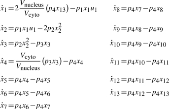
Consider performing a new measurement as illustrated earlier in Figure 1. The estimation of the measurement efficacy involves multiplying samples of the old posterior with new weights in order to estimate quantities for the situation after the experiment has been performed. When computing such a weighted average it is important to keep track of the quality of the estimation. When the posterior before and after a new experiment is very different, many of these sample weights will be very low and a large fraction of the samples will contribute only negligibly to the estimation of the new variance. It follows that such an estimate will be poor. We monitor this degeneracy by estimating the effective sample size (ESS) defined below (Del Moral et al., 2006).

(20)

We compute a distribution of ESS values (one for each incorporated sample) which we characterize by its median value. This ESS gives a measure for the quality of the sampling. In the case that the importance sampling distribution agrees well with the new posterior, it should scale linearly with the number of included samples. When the values for the ESS are very low then values obtained for the variance reduction can be inaccurate. It also implies that such a measurement would be very informative from an inferential perspective. This stems from the fact that the updated probability distribution would be much narrower. In such a case, it would be beneficial to perform the experiment and subsequently redo the MCMC step in such cases (for more information, see the Supplementary Materials).

Obtaining the PPDs as well as performing the experiment design is computationally expensive. For the former, model simulation time is a primary concern which can be significantly reduced by using compiled simulation code [see COPASI (Hoops et al., 2006); ABC-SysBio (Liepe et al., 2010); Potters Wheel (Maiwald and Timmer, 2008); Sloppy Cell (Brown and Sethna, 2003)]. Additionally more efficient sampling methods for obtaining such posteriors in high dimensional spaces are being developed (Girolami and Calderhead, 2011; Toni et al., 2009). For the experiment design part, the computational burden can be divided into two contributions. First is the sampling of the experiment space. Since each experiment constitutes a dimension in experiment space, densely sampling this space for a large number of experiments can become prohibitively time consuming. In this case, it may be required to resort to more sophisticated sampling techniques such as population MCMC or sequential Monte Carlo methods. One option we employ is to perform a fast initial sweep of the experiment space by sampling the LVR. Then in a subsequent step the actual SVR is computed for those samples that resulted in a large LVR. For a comparison of the LVR and SVR for one specific application, see the Supplementary Materials. Additionally, profiling the resampling step revealed that the distance calculations for the error model were most time consuming. Since this step exhibits a large degree of parallelism, the resampling step was also implemented to run on the GPU (using OpenCL), treating the resampling for each MCMC simultaneously. Even on a modest GPU (NVIDIA Quadro FX 580) this resulted in considerable speedup (see Supplementary Material).

As a last remark we would like to point out that if the goal of the experiment is to discriminate between models, alternative approaches (Skanda and Lebiedz, 2010) could be relevant to explore.

We proposed a flexible data-based strategy for OED. Where existing design criteria pertain to effectively constrain specific parameters or target the variance of predictions using model linearization (Casey et al., 2007; Faller et al., 2003; Rodriguez-Fernandez et al., 2006), this method is not limited to any specific error model or assumption regarding the parameter distribution. It enables the modeller to select specific predictions of interest that require decreased uncertainty thereby focus the experimental efforts in order to save time and resources. Furthermore, it allows the prediction of interest to be any quantity that can be obtained from simulations. An additional strength of the method is that multiple different measurements can be included in the design simultaneously in order to elucidate their combinatorial efficacy.

REFERENCES

- Brännmark C., et al. Mass and information feedbacks through receptor endocytosis govern insulin signaling as revealed using a parameter-free modeling framework. J. Biol. Chem. 2010;285:20171. doi: 10.1074/jbc.M110.106849. [DOI] [PMC free article] [PubMed] [Google Scholar]
- Brown K.S., Sethna J.P. Statistical mechanical approaches to models with many poorly known parameters. Phys. Rev. E. 2003;68:021904. doi: 10.1103/PhysRevE.68.021904. [DOI] [PubMed] [Google Scholar]
- Calderhead B., Girolami M. Statistical analysis of nonlinear dynamical systems using differential geometric sampling methods. J. R. Soc. Interface Focus. 2011;1:821–835. doi: 10.1098/rsfs.2011.0051. [DOI] [PMC free article] [PubMed] [Google Scholar]
- Casey F., et al. Optimal experimental design in an epidermal growth factor receptor signalling and down-regulation model. Syst. Biol. IET. 2007;1:190–202. doi: 10.1049/iet-syb:20060065. [DOI] [PubMed] [Google Scholar]
- Cedersund G., Roll J. Systems biology: model based evaluation and comparison of potential explanations for given biological data. FEBS J. 2009;276:903–922. doi: 10.1111/j.1742-4658.2008.06845.x. [DOI] [PubMed] [Google Scholar]
- Cowles M., Carlin B. Markov chain Monte Carlo convergence diagnostics: a comparative review. J. Am. Stat. Assoc. 1996;91:883–904. [Google Scholar]
- Del Moral P., et al. Sequential monte carlo samplers. J. Roy. Stat. Soc. B. 2006;68:411–436. [Google Scholar]
- Faller D., et al. Simulation methods for optimal experimental design in systems biology. Simulation. 2003;79:717. [Google Scholar]
- Geyer C. Practical markov chain monte carlo. Stat. Sci. 1992;7:473–483. [Google Scholar]
- Girolami M., Calderhead B. Riemann manifold Langevin and Hamiltonian Monte Carlo methods. J. Roy. Stat. Soc. B. 2011;73:123–214. [Google Scholar]
- Gomez-Cabrero D., et al. Workflow for generating competing hypothesis from models with parameter uncertainty. J. R. Soc. Interface Focus. 2011;1:438. doi: 10.1098/rsfs.2011.0015. [DOI] [PMC free article] [PubMed] [Google Scholar]
- Gutenkunst R.N., et al. Universally sloppy parameter sensitivities in systems biology models. PLoS Comput. Biol. 2007;3:e189. doi: 10.1371/journal.pcbi.0030189. [DOI] [PMC free article] [PubMed] [Google Scholar]
- Hasenauer J., et al. Parameter identification, experimental design and model falsification for biological network models using semidefinite programming. Syst. Biol. IET. 2010;4:119–130. doi: 10.1049/iet-syb.2009.0030. [DOI] [PubMed] [Google Scholar]
- Hoops S., et al. Copasia complex pathway simulator. Bioinformatics. 2006;22:3067. doi: 10.1093/bioinformatics/btl485. [DOI] [PubMed] [Google Scholar]
- Klinke D. An empirical Bayesian approach for model-based inference of cellular signaling networks. BMC Bioinformatics. 2009;10:371. doi: 10.1186/1471-2105-10-371. [DOI] [PMC free article] [PubMed] [Google Scholar]
- Kreutz C., Timmer J. Systems biology: experimental design. FEBS J. 2009;276:923–942. doi: 10.1111/j.1742-4658.2008.06843.x. [DOI] [PubMed] [Google Scholar]
- Kreutz C., et al. An error model for protein quantification. Bioinformatics. 2007;23:2747. doi: 10.1093/bioinformatics/btm397. [DOI] [PubMed] [Google Scholar]
- Kreutz C., et al. Likelihood based observability analysis and confidence intervals for predictions of dynamic models. 2011 doi: 10.1186/1752-0509-6-120. Arxiv preprint arXiv:1107.0013. [DOI] [PMC free article] [PubMed] [Google Scholar]
- Liepe J., et al. ABC-SysBio approximate Bayesian computation in Python with GPU support. Bioinformatics. 2010;26:1797. doi: 10.1093/bioinformatics/btq278. [DOI] [PMC free article] [PubMed] [Google Scholar]
- Maiwald T., Timmer J. Dynamical modeling and multi-experiment fitting with potterswheel. Bioinformatics. 2008;24:2037–2043. doi: 10.1093/bioinformatics/btn350. [DOI] [PMC free article] [PubMed] [Google Scholar]
- Neal R. Sampling from multimodal distributions using tempered transitions. Stat. Comput. 1996;6:353–366. [Google Scholar]
- Raue A., et al. Structural and practical identifiability analysis of partially observed dynamical models by exploiting the profile likelihood. Bioinformatics. 2009;25:1923. doi: 10.1093/bioinformatics/btp358. [DOI] [PubMed] [Google Scholar]
- Rodriguez-Fernandez M., et al. A hybrid approach for efficient and robust parameter estimation in biochemical pathways. Biosystems. 2006;83:248–265. doi: 10.1016/j.biosystems.2005.06.016. [DOI] [PubMed] [Google Scholar]
- Skanda D., Lebiedz D. An optimal experimental design approach to model discrimination in dynamic biochemical systems. Bioinformatics. 2010;26:939. doi: 10.1093/bioinformatics/btq074. [DOI] [PubMed] [Google Scholar]
- Swameye I., et al. Identification of nucleocytoplasmic cycling as a remote sensor in cellular signaling by databased modeling. Proc. Natl Acad. Sci. 2003;100:1028. doi: 10.1073/pnas.0237333100. [DOI] [PMC free article] [PubMed] [Google Scholar]
- Tiemann C., et al. Parameter adaptations during phenotype transitions in progressive diseases. BMC Syst. Biol. 2011;5:174. doi: 10.1186/1752-0509-5-174. [DOI] [PMC free article] [PubMed] [Google Scholar]
- Toni T., et al. Approximate bayesian computation scheme for parameter inference and model selection in dynamical systems. J. Roy. Soc. Interface. 2009;6:187–202. doi: 10.1098/rsif.2008.0172. [DOI] [PMC free article] [PubMed] [Google Scholar]
Associated Data
This section collects any data citations, data availability statements, or supplementary materials included in this article.