Picking ChIP-seq peak detectors for analyzing chromatin modification experiments

Abstract

Numerous algorithms have been developed to analyze ChIP-Seq data. However, the complexity of analyzing diverse patterns of ChIP-Seq signals, especially for epigenetic marks, still calls for the development of new algorithms and objective comparisons of existing methods. We developed Qeseq, an algorithm to detect regions of increased ChIP read density relative to background. Qeseq employs critical novel elements, such as iterative recalibration and neighbor joining of reads to identify enriched regions of any length. To objectively assess its performance relative to other 14 ChIP-Seq peak finders, we designed a novel protocol based on Validation Discriminant Analysis (VDA) to optimally select validation sites and generated two validation datasets, which are the most comprehensive to date for algorithmic benchmarking of key epigenetic marks. In addition, we systematically explored a total of 315 diverse parameter configurations from these algorithms and found that typically optimal parameters in one dataset do not generalize to other datasets. Nevertheless, default parameters show the most stable performance, suggesting that they should be used. This study also provides a reproducible and generalizable methodology for unbiased comparative analysis of high-throughput sequencing tools that can facilitate future algorithmic development.

INTRODUCTION

ChIP-Seq is a massively parallel sequencing technique that has now become the leading tool for studying the dynamic interplay between transcriptome and epigenome (1). It enables profiling of the genomic locations of immunoprecipitated DNA fragments bound by transcription factors, epigenetic marks or other proteins at an unprecedented resolution. In a ChIP-Seq experiment, the protein of interest is initially cross-linked to DNA. The cross-linked chromatin is then fragmented (e.g. by sonication or micrococcal nuclease, MNase, digestion) and enriched by immunoprecipitation using specific antibodies. Cross-links are reversed and the enriched DNA fragments are then amplified and sequenced using massively parallel sequencing technologies. The resulting sequence reads are then mapped to the corresponding genome sequence for further analysis. To estimate baseline enrichment, genomic DNA is sequenced without antibody enrichment (total input). In parallel, non-specific binding can be estimated using control antibodies, such as IgG.

There are several technical aspects of a ChIP-Seq experiment that can impact the quality of the obtained data, including but not limited to antibody specificity, cell type, selection of negative control, chromatin fragmentation techniques and sequencing protocol (e.g. library construction, length of the reads, single or paired-end experimental protocol and sequencing depth). Moreover, the identity of the protein or histone mark of interest can affect the spatial distribution of protein–DNA interactions. For example, histone marks span broad genomic regions, from one nucleosome (∼150 bp) to large chromosomal domains, with no evident association to specific sequence motifs (2), while transcription factors typically bind to well-defined sequence-specific regions in the genome.

As ChIP-Seq protocols and the sequencing technology have matured over the years, numerous genome-wide datasets have been generated and the quality of these datasets has significantly improved with deeper coverage. These advances have been accompanied by a similarly rapid development of computational tools to analyze these datasets. In particular, algorithmic performance has improved from low to high sensitivity (3) by using better combinations of signal processing strategies, such as correction of sequencing biases, calibration of signal from each experimental lane, filtering of PCR artifacts or strand imbalances and fine-tuning of the parameters of analysis.

Despite the apparent abundance of computational tools, the need for a simple, parameter-free, yet robust pipeline warrants development of versatile approaches that are capable of locating binding events with high sensitivity and specificity in diverse datasets. These approaches are required to detect events in multiple datasets that may have varying length scales, intensities and gaps from other events. The prediction and localization of enriched events in ChIP-Seq data are still not straightforward computational tasks due to the already mentioned biological and experimental variations and other poorly characterized factors (e.g. chromatin compaction, proximity of adjacent binding sites). Moreover, each of the available peak detectors addresses only a certain set of these aspects, affecting the number and characteristics of reported events. For example, some of the ChIP-Seq algorithms are fine-tuned to work with specific proteins while others are better suited to analyze epigenetic marks and require a number of parameters to be explored by the user (4,5).

The development of ChIP-Seq algorithms has equally been hindered by limitations in objective benchmarking standards, resulting in limited efforts to compare their performances (3). An important aspect in comparative benchmarking of ChIP-Seq event detectors is to have sizeable validation sets that are not selected from the predictions of one single algorithm and are obtained by independent quantitative PCR (qPCR) experiments (the gold standard in the field). Choosing a set of validation sites for a comparative study requires a careful design and therefore we developed a ChIP-Seq specific protocol based on our general Validation Discriminant Analysis (VDA) approach (6). This allowed us to perform an objective comparison between 15 ChIP-Seq algorithms using histone modification datasets.

In this study, we introduce Qeseq, a novel non-parametric ChIP-Seq event-finding algorithm, and systematically compare its performance with 14 other programs in histone modification datasets. Using an approach that integrates selection of validation sites and ranking of algorithmic performance in an unbiased fashion, we show that Qeseq is a robust computational tool for analyzing epigenetic datasets. We also demonstrate through an extensive parameter optimization effort that default parameters typically are good choices as they stand out in terms of their stability in algorithmic performance.

MATERIAL AND METHODS

Publicly available ChIP-Seq datasets with qPCR validations

In the present study, we used publicly available histone modification ChIP-Seq datasets for lysine 4 tri-methylation of histone H3 in mouse embryonic stem (ES) cells (ES.H3K4me3) (7), lysine 27 tri-methylation of histone H3 in mouse ES cells (ES.H3K27me3) (7) and in mouse muscle cells (MYO.H3K27me3.GM and MYO.H3K27me3.MT), and lysine 36 tri-methylation of histone H3 in mouse muscle cells (MYO.H3K36me3.GM) (8). qPCR validations were available for each of the above ChIP-Seq datasets. Additional information on the datasets and their qPCR validations is shown in Tables 1 and 2, respectively.

Table 1.

Characterization of the histone modification ChIP-Seq datasets in terms of the number of ChIP and control reads

Histone modification	ChIP reads	Control reads
ES.H3K27me3	6 537 926	715 231
ES.H3K4me3	8 850 116	715 231
MYO.H3K27me3.GM	29 694 722	32 866 230
MYO.H3K27me3.MT	28 538 546	27 406 448
MYO.H3K36me3.GM	25 322 796	32 866 230

Table 2.

Characterization of the qPCR validation sites

Histone modification	Positives	Negatives	Total	Source
ES.H3K27me3	17	14	31	(7)
ES.H3K4me3	19	14	33	(7)
MYO.H3K27me3.GM	70	30	100	(8)
MYO.H3K27me3.MT	65	35	100	(8)
MYO.H3K27me3.GM.VDA	145	52	197	VDA validated sites
MYO.H3K36me3.GM.VDA	71	23	94	VDA validated sites

VDA selected qPCR-validated datasets

To rank performances of available ChIP-Seq algorithms, we designed two novel validation datasets (H3K27me3.GM.VDA and H3K36me3.GM.VDA) using the VDA approach (Supplementary Notes C and Results section). qPCR validation sites were considered to be positive or negative according to empirical ChIP-qPCR comparing several wild type and knock-out cell lines (9). These tests, showed that under the ChIP conditions used (buffers, washes etc), with three biological replicates, a minimum cutoff for a positive site of 0.05% enrichment over total input eliminated ≥98% of false positive events (P. Asp and B. Dynlacht, unpublished results). This value is the equivalent of using 5 ng of total chromatin as the qPCR template. Loci where the enrichment of the IgG control ChIP over total input control was found >0.05% in two independent ChIP experiments were removed from the study due to high non-specific background. ChIP-qPCR analysis of the VDA selected sites using the criteria described above generated 197 validated sites for the MYO.H3K27me3.GM.VDA dataset and 94 validated sites in the MYO.H3K36me3.GM.VDA; 291 validation sites in total (Table 2).

Algorithms

We considered Qeseq and 14 other state-of-the-art ChIP-Seq tools. We initially tested Qeseq and 10 other algorithms: CCAT (10), ChIPDiff (11), ERANGE (12), FindPeaks(13), FSeq (14), MACS (15), PeakSeq (16), QuEST (17), SICER (18) and SISSRs (19). For completeness, we added four algorithms to the comparative study that were not available when we designed the validation experiments: RSEG (20), Swembl (21), TPIC (22) and W-ChIPeaks (23) (Supplementary Table S1a, b and Supplementary Notes A).

Evaluation of algorithmic performance using qPCR validation experiments

ChIP-Seq datasets were analyzed with these 15 algorithms using the default or recommended settings. Predicted events were compared to the sets of validated sites. All algorithms were run using total input as control, when required. The performance of each algorithm was assessed using the area under the receiver operating characteristic curve (AUCROC) measure, which for binary predictors (whether DNA binding occurs or not) is reduced to the balanced accuracy [Equation (3) in Results section]. To account for the loss of resolution due to the increased presence of non-mononucleosomal fragments in the qPCR validation experiments (Supplementary Notes B and Supplementary Tables 5–6), we added flanking regions to the boundaries of qPCR-validated sites: 150 bp for histone marks according to the reported average fragment size. A predicted event was considered a True Positive if it was validated by qPCR as a positive site, or a False Positive if it was not validated by qPCR. qPCR validated positive sites were considered False Negatives if there was no predicted event; similarly, True Negatives were qPCR validated negative sites with no predicted event.

RESULTS

Qeseq

Algorithm design

The Qeseq algorithm analyzes aligned sequence reads from ChIP-Seq data and identifies regions that show a significant enrichment of ChIP signal relative to the control. Two design choices guided our algorithmic development: (a) a parameter-free easy-to-use model combined with (b) high specificity and improved sensitivity when measuring algorithmic performance. Reflecting these goals, the algorithm consists of three main modules: relative enrichment estimation, cluster detection and filtering of artifacts (Supplementary Figure S1). Qeseq iteratively cycles through its first two modules by removing detected clusters and reevaluating enrichment and cluster detection on the remaining signal until no new events are detected. The third module is used once to prune artifacts from the results. The average length of DNA fragments is the only parameter required from the user, which is determined during ChIP-Seq library preparation and is verified experimentally as part of most protocols.

Relative enrichment estimation

This module estimates the local enrichment of ChIP signal relative to the control from the raw data (Supplementary Figures S2–S5). The underlying assumption is that the density of sequencing reads can be used to determine this enrichment. Qeseq generates smooth profiles for the ChIP sample and control signal separately on each chromosome using kernel density estimation (KDE) with fixed bandwidth (24). We implemented the Gaussian KDE (GKDE) in Qeseq (Supplementary Figures S2A, S3A, S4 and S5), although other choices of kernel yield very similar results (Supplementary Figures S2B, C, D, 3B, C and D). In particular, we define the genomic position of a sequenced read as its start site, and then for a genomic position x, the experimental density (D) is defined as follows:

(1)

where is the kernel bandwidth in base pairs, n is the total number of reads within the chromosome, and each x_j is the genomic position of a sequenced read within 3h from x. The densities (D) are computed separately for the ChIP and the control lanes, such that both densities are estimated at the genomic positions of reads from the ChIP lane. For the ChIP signal x_j represents the genomic positions of ChIP reads, and for the control signal x_j represents the genomic positions of control reads. Because the ChIP and control densities are evaluated within 3h of the position x of the ChIP reads, the control lane might not have reads in this genomic region. 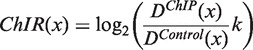We accounted for this bias by adding a pseudo-count of to the control density. We defined the enrichment of the ChIP signal with respect to the control as the ChIP to control log-ratio (ChIR) of the two densities. Qeseq computes the ChIR at the genomic positions x of each read in the ChIP lane as follows:

(2)

where and are the ChIP and control densities, respectively, and k is a calibration coefficient defined as 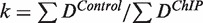(Supplementary Figures S4 and S5).

Event detection

At the genomic position of each ChIP read, we applied the two-sample Cramér-von Mises test (25,26) to two vectors of the same length representing the empirical and theoretical ChIR distributions to assess significance at the level of α = 0.05. Our theoretical distribution represents the limit of the null distribution when the sequencing coverage is very large. In detail, we compared the distribution of ChIRs within 3h of the position x of the ChIR of interest with the theoretical null distribution with zero mean and zero variance. We assessed the significance of the deviation of the ChIR from the theoretical null distribution at all the genomic positions covered in the ChIP lane (Supplementary Figures S6D and S7D).

A candidate event was then defined as a contiguous genomic region where all the nucleotides within this interval are within a distance of 3h from a significantly enriched ChIR. Using this definition we derived the boundaries of each candidate event (Supplementary Figures S6E and S7E).

To test the significance of each candidate event we again used the Cramér-von Mises non-parametric test, but this time it is not applied at the nucleotide level. Rather, this second test assesses whether the empirical distribution of ChIRs within the boundaries of a detected candidate event, is significantly different from the theoretical distribution centered at zero (using the cutoff α = 0.01). Only significant candidate events are retained as positive events (Supplementary Figures S6G and S7G).

We note that the first test used to define candidate events has a less stringent threshold (α = 0.05), which allowed us to improve sensitivity, especially in noisy extended regions, where the significance of individual ChIRs could be hindered by suboptimal coverage. Additionally, we note that the Cramér-von Mises test can detect differences in distributions with higher statistical power than the commonly used two-sample Kolmogorov-Smirnov test (25).

Recalibration

The expected ChIR value of event-free regions should be zero. However, the presence of real binding events generates a heavier right tail in the distribution of the ChIR. We therefore recalibrated the coefficient k [Equation (2)] so that, after masking genomic regions with candidate events, the ChIR distribution for each chromosome was centered at zero (Supplementary Figures S8 and S9). We iteratively repeated calibration, position and candidate event significance assessments on the remaining genomic regions until no new events were detected.

Filtering of artifacts

In ChIP-Seq signals, experimental noise and sequencing artifacts can contribute to the detection of false events. A common assumption is that reliable candidate events have substantial average enrichment and are characterized by roughly equal number of reads from both DNA strands. To ensure that reported events possess both these qualities, Qeseq removes events that are enriched in the control lane relative to a signal constructed by replacing the read density of every candidate event with a uniform distribution, representing the average read density across all events. This procedure identifies and removes all sites associated with PCR amplification artifacts as well as spurious or non-specific enrichment (Supplementary Figure S10). Furthermore, Qeseq removes events with a ratio >2:1 between the number of reads mapped to the positive (negative) and to the negative (positive) DNA strands, when the total number of reads in the event is large (Supplementary Figure S11). Such events can be the result of incorrect mapping of sequences from repeat elements, or non-specific immunoprecipitation (27).

Additional characteristics of Qeseq

Qeseq provides both browser extensible data (BED) and sequence graph data (SGR) output formats to facilitate visualization in genome browsers. The default output of Qeseq consists of useful information for each event including the number of reads within the event mapped to each strand, the average ChIR and the event P-value. All peaks that are filtered out are stored in a separate ‘false positive events’ file.

Qeseq is implemented in C++ and it is freely available at http://sourceforge.net/projects/klugerlab/files/qeseq/

Performance comparison

Unbiased evaluation of algorithmic performance

Previous comparative studies measured algorithmic performance by assessing the number of events that are correctly classified in the test dataset based on specific qPCR validation datasets (4,5). The most commonly used measure of performance in these studies is the area under the receiver operating characteristic curve (AUCROC), which for a binary predictor i corresponds to the balanced accuracy:

(3)

These earlier comparative studies, however, did not take into account that sampling biases might have occurred in the selection of validation sites. In fact, an unbiased estimate is necessary for validation sets generated using a biased strategy, such as the VDA approach.

We therefore sought to define an unbiased estimate of algorithmic performance (Supplementary Notes C) that is independent of sampling biases. In detail, we derived a corrected AUCROC formula for an algorithm i that estimates the number of nucleotides in the genome that would be correctly classified as present (or absent) in a binding event:

(4)

These estimates were computed after partitioning the genome into sets of nucleotides sharing the same fingerprint, i.e. a binary vector [A₁, A₂, … , A_n] where A_i is 1 if the nucleotide was predicted as part of a binding site by algorithm i or 0 otherwise (Supplementary Notes C). The numbers of nucleotides expected to be true positives , true negatives , positives and negatives were estimated as (6):

(5)

where to each nucleotide we assigned a fingerprint defined as a binary vector [A₁, A₂, … , A_n] where A_i is 1 if the nucleotide was predicted as part of a binding site by algorithm i or 0 otherwise; R is the total number of nucleotides in the genome; W is the subset of the 2ⁿ possible fingerprints, which consists of the union of all fingerprints associated with the nucleotides covered in the validation experiment; C_k is the number of nucleotides that have fingerprint k; P_k and N_k are the number of nucleotides associated with the fingerprint k that were experimentally validated as positives and negatives respectively; and TP_ik and TN_ik are the number of nucleotides of fingerprint k that are correctly identified as true positives and true negatives by a given algorithm. It follows from this definition that our unbiased estimate is not significantly different from previous biased estimates when the validation set is chosen randomly.

Using the corrected , , and defined in Equation (4), we also derived unbiased estimates of precision, recall, true negative rate and F-measure (28) (Figure 1 and Supplementary Table S2). We found that our unbiased AUCROC formula is robust across datasets. When comparing algorithmic performance lower variance is achieved (Figure 2).

Figure 1.

Sensitivity and specificity in qPCR validated histone modification datasets. Algorithms are in order of publication. A LOESS estimator has been added to facilitate visualization. (A) Specificity statistics of 15 ChIP-Seq algorithms remain almost invariant over time in the range of 0.9–1 in all four histone modification datasets. The minor decrease in specificity in the newer algorithms is due to less restrictive detection procedures that allow a significant improvement in sensitivity (cf. panel B). (B) Sensitivity statistics of 15 ChIP-Seq algorithms shows an increasing trend over time in all four datasets.

Figure 2.

Correlation between biased and unbiased AUCROC estimators in qPCR validated histone modification datasets. (A) Estimation of performance using independent validation datasets (MYO.H3K27me3.GM and MYO.H3K27.GM.VDA) derived from the same experiment showed higher reproducibility when using the unbiased AUCROC estimator (black dots). The biased AUCROC statistics (red dots) consistently produced higher estimates for the MYO.H3K27me3.GM. Proximity of a dot to the grey diagonal line indicates that the AUCROC estimates of a given algorithm are similar in two independent validation datasets (B) Heatmap of correlations between performance profiles of six histone modifications. Each profile is a 15D vector representing the performance of the 15 ChIP-Seq algorithms. Colors indicate the degree of correlation, where red is positive correlation, green is negative correlation and white represents no correlation. Strong anti-correlations between performance profiles of different histone marks are observed when we use the biased AUCROC estimator (orange square). In contrast, the use of the unbiased AUCROC estimator leads on average to higher correlations between the performance profiles (blue square).

Performance analysis based on existing qPCR validations using unbiased AUCROC measure

We initially assessed the performance of each algorithm using publicly available qPCR validation datasets (Table 2). Our unbiased AUCROC measure [Equation (4)] indicated differences between algorithms, suggesting that on average the most recent algorithms had improved performance (Figure 3A and Tables 3 and 4). Using the existing histone qPCR validation datasets, ChIPDiff, FindPeaks FSeq, Qeseq, RSEG, SWEMBL and TPIC have AUCROCs > 0.8 in the majority of cases (Figure 3A). On average, in the four existing datasets the top performing algorithms had nearly identical AUCROCs: RSEG (average AUCROC = 0.87), Qeseq and FindPeaks (both with average AUCROC = 0.85).

Figure 3.

Comparison of unbiased AUCROC performance estimates in existing and novel qPCR validated histone modification datasets. Algorithms are in order of publication. LOESS estimators have been added to facilitate visualization. (A) AUCROC statistics of the 15 ChIP-Seq algorithms sorted according to their time of publication shows incremental improvements in existing qPCR validated histone modification datasets (MYO.H3K27me3.GM, MYO.H3K27me3.MT, ES.H3K4me3 and ES.H3K27me3). The lines indicate that over time algorithms achieved better performance. (B) AUCROC statistics of the 15 algorithms sorted according their time of publication shows incremental improvements in novel qPCR validated histone modification datasets (MYO.H3K27me3.GM.VDA and MYO.H3K36me3.GM.VDA). The lines indicate that over time algorithms achieved better performance.

Table 3.

Performance analysis for each algorithm using the default settings in histone modification datasets based on unbiased AUCROC statistic

Datasets/Algorithms	CCAT	ChIPDiff	ERANGE	FindPeaks	FSeq	MACS	PeakSeq	Qeseq	QuEST	RSEG	SICER	SISSRS	SWEMBL	TPIC	W-ChiPeaks
MYO.H3k27me3.GM.VDA	0.8232	0.8331	0.5038	0.8427	0.7638	0.6583	0.6500	0.8378	0.5011	0.8591	0.5000	0.5089	0.8124	0.8025	0.5085
MYO.H3k36me3.GM.VDA	0.6223	0.6696	0.5000	0.4610	0.6140	0.6148	0.5483	0.6722	0.5000	0.6217	0.6212	0.5002	0.6037	0.6200	0.5000
MYO.H3k27me3.GM	0.8002	0.7879	0.5003	0.7987	0.7931	0.5980	0.6229	0.7991	0.5000	0.7991	0.5000	0.5010	0.7998	0.7993	0.5046
MYO.H3k27me3.MT	0.7355	0.7340	0.5000	0.7350	0.7128	0.5394	0.5590	0.7319	0.5000	0.7354	0.5000	0.5002	0.7362	0.7355	0.5015
ES.H3K4me3	0.8413	0.8426	0.8088	0.8738	0.9742	0.9630	0.4951	0.9940	0.6697	0.9972	0.9970	0.5000	0.9032	0.9814	0.8373
ES.H3K27me3	0.5027	0.9172	0.5826	1.0000	0.8366	0.6757	0.7294	0.8703	0.5551	0.9454	0.8853	0.5000	0.8747	0.8607	0.7185

Table 4.

Average performance of each algorithm using the default settings in histone modification datasets based on unbiased AUCROC statistic

Datasets/Algorithms	CCAT	ChIPDiff	ERANGE	FindPeaks	FSeq	MACS	PeakSeq	Qeseq	QuEST	RSEG	SICER	SISSRS	SWEMBL	TPIC	W-ChiPeaks
AVERAGE ALL HISTONE DATASETS	0.7209	0.7974	0.5659	0.7852	0.7824	0.6749	0.6008	0.8175	0.5377	0.8263	0.6672	0.5017	0.7883	0.7999	0.5951
AVERAGE VDA DATASETS	0.7227	0.7513	0.5019	0.6518	0.6889	0.6366	0.5991	0.7550	0.5006	0.7404	0.5606	0.5046	0.7081	0.7112	0.5042
AVERAGE EXISTING DATASETS	0.7199	0.8204	0.5979	0.8519	0.8292	0.6940	0.6016	0.8488	0.5562	0.8693	0.7206	0.5003	0.8285	0.8442	0.6405

VDA-based design of novel validation datasets

Experimentally validated histone modification datasets are scarce, and most algorithms have been trained and tested on specific and small datasets (Supplementary Notes C). In order to overcome this limitation, we designed two novel extensive histone modification qPCR datasets.

For a fair comparison between algorithms we sought to select validation sites by using our VDA approach (Supplementary Notes C.I), such that the resulting validation dataset consists of a subset of sites with higher discriminative power than a random subset. Specifically, VDA maximizes the minimum number of discordant predictions between any pair of algorithms (i.e. we want to choose validation sites such that the minimal discrepancy between any pair of algorithms is maximized). This procedure enables a more reliable ranking of algorithmic performance than using random subsets from the list of all available sites (6).

To select validation sites we initially implemented the genome segmentation protocol (Supplementary Notes C.II) based on the predictions obtained for MYO.H3K27me3.GM with CCAT, ChIPDiff, ERANGE, FindPeaks, FSeq, MACS, PeakSeq, Qeseq, QuEST and SISSRs. Myoblast H3K27me3 ChIP-qPCRs were performed for 115 sites and 99 of these sites were successfully characterized as H3K27me3 positives or negatives (see ‘Materials and Methods’ section), resulting in 88 positives and 11 negatives. In addition, to further discriminate between the top performing algorithms we designed a second set of validation sites selected by applying the ChIP-Seq VDA protocol to predictions from CCAT, FSeq, MACS, PeakSeq and Qeseq in MYO.H3K27me3.GM data. This increased the size of the MYO.H3K27me3.GM.VDA validation set with an additional 98 sites, which, together with the first set, comprised 197 sites. For these additional 98 sites, we implemented the clean-sites protocol (Supplementary Notes C.III) to define candidate sites that improve robustness to the loss of resolution introduced by conventional qPCR. To avoid possible bias from using only one histone mark for testing, we applied the clean-sites protocol (Supplementary Notes C.III) to the predictions obtained for another mark, MYO.H3K36me3.GM using CCAT, FSeq, MACS, PeakSeq and Qeseq. 94 sites (out of 114) were successfully validated by ChIP-qPCR.

Comparison of algorithmic performance using VDA datasets

In the H3K27me3.GM.VDA dataset, RSEG (AUCROC = 0.86), FindPeaks (AUCROC = 0.84) and Qeseq (AUCROC = 0.84), showed the highest AUCROCs (Figure 3B and Tables 3 and 4), largely outperforming all other algorithms. Performances were lower in the H3K36me3.GM.VDA dataset where the leading algorithms were Qeseq (AUCROC = 0.67) and ChIPDiff (AUCROC = 0.67) (Figure 3B and Tables 3 and 4). On average, in these two novel validation datasets, Qeseq (average AUCROC = 0.75) and CCAT (average AUCROC = 0.72) had the best performance along with two HMM-based algorithms, ChIPDiff (average AUCROC = 0.75) and RSEG (average AUCROC = 0.74).

Exploration of the parameter space of ChIP-Seq algorithms

Design of parameter space exploration

Most algorithms have a number of parameters that can be set by the user (Table 5). For any algorithm, exploring the parameter space to improve performance is time-consuming and prone to over-fitting (29). Moreover, it is difficult to predict how results may vary as parameter values are changed. In addition to our analysis on default settings, conducted under the assumption that developers have extensively tested their programs to ensure best average performance, we also explored the parameter space of all the parametric algorithms considered in our study (Table 5). We sought to obtain an overview of the effects of different parameters on the performance, stability and monotonicity of such changes. For each algorithm, we modified one parameter at a time up to two orders of magnitude in logarithmic scale around the default value, resulting in effectively comparing 315 models, each applied to six epigenetic datasets. This is an unprecedented effort in the characterization of parameter space of bioinformatics algorithms for comparative purposes.

Table 5.

Summary of parameter space explored for each algorithm

Algorithms	Parameters explored
CCAT	Bootstrap pass: number of passes in the bootstrapping process
	Minimum count: minimum number of read counts at the peak
	Minimum score: minimum score of normalized difference
	Moving Step: step of window sliding
	SlidingWinSize: size of sliding window
ChIPDiff	MaxIterationNum: maximum number of iterations
	MinRegionDist: minimum distance between two histone modification regions
	MinFoldChange: threshold for fold change
	MinP: threshold for confidence
	MaxTrainingSeqNum: maximum number of sequences for training.
ERANGE	Autoshift: calculate a ‘best shift’ for each region
	Shiftlearn: pick the best shift based on the best shift for strong sites using the parameter
	Notrim: turns off region trimming
	NoDirectionality: the fraction of + strand reads required to be to the left of the peak
	Minimum: minimum number of reads within the region
	Ratio: sets the minimum fold enrichment
	Shift: shift reads by half the expected fragment length
	Space: sets the maximum distance between reads in the region
FindPeaks	DistType: type of distribution used
	Iteration: Monte-Carlo FDR for estimating background noise
	MinCoverage: modifies the distribution to remove contributions below the supplied height
	SubPeaks: turns on the subpeaks module, to perform peak separation
	Trim: float value is used to determine the amount of the shoulder of each peak retained
	WindowSize: size of scanning window
FSeq	FeatureLength: feature length
	Threshold: standard deviations
MACS	MFold: regions within MFOLD range of high-confidence enrichment ratio against background to build model
	NoLambda: if True, MACS will use fixed background lambda as local lambda for every peak region
	NoModel: whether or not to build the shifting model
	PValue: P-value cutoff for peak detection
PeakSeq	MaxRegExt: largest region for which the extended region is evaluated
	PvalThresh: threshold P-value for a peak
	Region: amount on each side that regions are extended when extended regions are used
	BinSize: bin size for doing linear regression
	WPerC: number of windows per chromosome
	WSize: window size for scoring
	MinFDR: required false discovery rate
	MaxCount: maximum number of reads using the same starting nucleotide
	NSims: number of simulations per window to estimate FDR
	MaxGap: maximum gap allowed between peaks for them to be merged together
Qeseq	There are no parameters to change.
QuEST	We tried to change two parameters: quick-window scan and calibrate peak shift. The output format changed, rendering the results of these parameter changes not applicable to our study.
RSEG	Bin: an integer to specify the size of bins used in the program
	Desert: an integer value so that if the size of a deadzone is larger than this value, the deadzone is ignored from subsequent analysis
	Distribution: emission distribution used in the program to model read counts
	Probability: minimum probability value
	Iteration: maximum number of iterations for HMM training
SICER	WindowSize: size of the windows to scan the genome width
	GapSize: allowed gap in base pairs between islands
	FDR: false discovery rate controlling significance
SISSRS	DirReads: number of ‘directional’ reads required within certain number of base pairs on either side of the inferred binding site
	Pvalue: p-value threshold
	Window: size of the overlapping/sliding scanning window
SWEMBL	Penalty gradient (p)
	Penalty gradient (p) after gap of certain size (d)
	Fragment extension: extend fragment in the direction of the read up to a certain length
TPIC	Width: width of interval used to calculate local rate γ (t)
	D: parameter used in discretizing γ
	Min_Region_Length: size of the overlapping/sliding scanning window
W-ChiPeaks	Bin size
	FDR: false discovery rate

Parameter change affects length scale of detected binding events

As recently reported (30), the characteristics of binding events reported by different algorithms vary significantly. We found that at default settings most algorithms had an invariant distribution of event lengths, regardless of the dataset (Figure 4 and Supplementary Table S3a). We hypothesized that for these algorithms the characteristic distribution of event lengths is a function of a subset of parameters. We therefore examined each algorithm and explored how the length scales varied by changing one parameter at a time. We analyzed the MYO.H3K27me3.GM dataset and observed that the parametric variants of each algorithm typically clustered together (Figure 5). Within the CCAT, ERANGE and RSEG clusters, however, we noticed that there were parameters that substantially affected the distributions of event lengths. As expected, these changes were associated with parameters that reduce resolution, thus increasing the length of predicted events. These parameters were for instance ERANGE's space, RSEG's Gauss distribution, and CCAT's sliding window size parameters.

Figure 4.

Distribution of lengths of binding events detected by 15 ChIP-Seq algorithms in histone modification datasets. For each algorithm and for each dataset the distribution of site lengths is displayed as a density heatmap. The empirical probability of an event length is shown in greyscale, with darker grey indicating higher probability. Algorithms such as MACS and SISSRs exhibit a short range of event lengths. Other algorithms, such as ChIPDiff and QuEST have a broader spectrum of site lengths. Default settings were used in all algorithms.

Figure 5.

Comparison of length scale characteristics of binding events detected by 315 parametric models in MYO.H3K27me3.GM.VDA dataset. For each parametric model the distribution of site lengths is displayed as a density heatmap. The empirical probability of an event length is shown in greyscale, with darker grey indicating higher probability. The parametric variants of each algorithmic model are grouped together to simplify visualization. Most parameters in each algorithm do not affect the length distribution of the detected events.

Parameter change affects the number of detected binding events

To explore the stability of parameters, we performed Principal Component Analysis (PCA) on a 315-by-6 matrix of the number of detected events to effectively visualize similarities and dissimilarities between all the 315 models. Since we sought to examine how varying one parameter impacts the number of detected events, we projected the data onto the two leading principal components and drew lines connecting between models derived by changing a single parameter of a given algorithm (Figure 6A and Supplementary Table S3b). For a given algorithm, trajectories stem from the default setting. Each trajectory corresponds to a single parameter (Supplementary Notes D). As Qeseq has no parameters to be explored, its PCA representation is a point corresponding to the default settings.

Figure 6.

PCA of the number of detected events and AUCROC performances of 315 ChIP-Seq models in six histone modification datasets. (A and B) Data was projected onto its first two principal components using standard PCA. Each of the 15 ChIP-Seq algorithms is shown with a distinctive color. For each algorithm, there are several trajectories each representing the span of the parametric variants obtained by changing a single parameter. All the trajectories stem from the default setting. (A) PCA was performed on the number of detected binding events. Long trajectories reflect parametric instability as seen for example in, the trajectories of SISSRs, CCAT and ERANGE. (B) PCA was performed on the AUCROC statistics. Algorithms whose performance is stable to fine-tuning of parameters have short trajectories, for example TPIC and SWEMBL.

Stable parameters have very short and almost linear trajectories. Therefore, we hypothesized that the difference between algorithms would be larger than the difference between the parametric variants of the same algorithm. On the contrary, we found that most parameter trajectories traversed large regions (Figure 6A) and the number of detected binding events across the ChIP-Seq datasets varied significantly (spanning more than four orders of magnitude) between algorithms and between parametric variants of the same algorithm. Overall, this suggests that the algorithms could not fully capture the multi-scale characteristic of a given histone mark.

Parameter change affects algorithmic performances across datasets

We further investigated the stability of performance as parameters were tuned. A desirable property of a parametric model is that the differences in performance between its parametric variants are proportionately related to the differences in the parameter, such that small deviations from the default setting would result in small changes in performance.

To compare performances of the 315 models across six histone modification datasets we applied PCA to a 315-by-6 matrix of unbiased AUCROC measures to display the dissimilarities between these models (Figure 6B). Additionally, we used a PCA biplot (Figure 7), which simultaneously displays the multidimensional models and histone modification datasets in 2D (31,32). PCA allowed us to inspect which algorithmic models and parameter choices are grouped together, and locate a region in this space with the top performing models across all datasets. Moreover, with the aid of the biplot approach we could observe the approximated performance of each model in each dataset (Supplementary Notes D.III).

Figure 7.

Biplot of the performances of 315 ChIP-Seq models in six histone modification datasets. Data was projected on its two principal components using standard PCA techniques. In addition, the vectors corresponding to the six histone modification datasets were added as arrows. All parametric models from 15 ChIP-Seq algorithms are represented by dots identifiable by their distinctive colors. In addition, a density heatmap was added to the background and supplied by isoclines at 25% of the total density. The density heatmap was computed using a 2D Gaussian kernel with bandwidth of 0.05 in the principal component units. Few algorithms (RSEG, SWEMBLE and CCAT) correspond to parametric models that occupy small well-defined regions of the PCA space. Other algorithms show a continuous spread of performances (Erange, W-ChIPeaks); others, like SISSRs have multimodal density distributions, as clearly shown by the presence of multiple disconnected circles.

We observed instability in algorithmic behavior, where small changes in the choice of parameters often resulted in large deviations in performance, most notably for ERANGE, and FindPeaks (Figure 6B). For example, when we modified the Subpeaks parameter of FindPeaks in the MYO.H3K27me3.GM.VDA dataset by one order of magnitude, we observed that the AUCROC changed from 0.77 to 0.60 (Supplementary Table S4). Changing ERANGE's shift parameter by one order of magnitude in the ES. H3K4me3 dataset induced AUCROC to drop from 0.80 to 0.50 (Supplementary Table S4). These parameters impact how short events with few reads are clustered together into longer events. As a result, we found high correlation between the value of these parameters and the number of false negatives.

We also observed models generated by the parametric variants of the CCAT algorithm fall into a cluster. The performance ranking of the CCAT variants is high in the MYO datasets. Similarly, the variants of the MACS algorithm are highly ranked in the ES cell datasets. These results suggest that the different underlying design choices of these two algorithms capture distinct properties of the signals. Importantly, five algorithms (Qeseq, TPIC, RSEG, SWEMBL and FindPeaks) were high performers across all datasets.

The choice of optimal parameters varied across different datasets

A natural way to optimize parameters is by using minimization procedures. However, as described above we observed that changes of some parameters led to strong changes in performance. Although fine-tuning could still be performed by exhaustive or heuristic search of the parameter space, the critical question is whether a model obtained by such a procedure is generalizable to multiple types of similar signals. Fitting parameters for a single dataset requires extensive validation experiments: desirably, fine-tuning should be done once and its results confidently used for all other related datasets.

To determine whether fine-tuning is a recommended step for analysis of a new ChIP-Seq dataset, we examined if we could identify a best set of parameters for each algorithm such that the fine-tuned version would consistently achieve higher performance than the default settings in all datasets. We investigated this in two ways: (i) we checked whether fine-tuning of a single parameter could improve the performance in each epigenetic dataset, and (ii) we explored whether, for each algorithm, the optimal parameter choice in one dataset consistently improved (not necessarily optimized) algorithmic performance in all the other datasets with respect to the default parameter.

When we addressed point (i) above, we noticed that for algorithms for which the default parameters were not the best across all datasets, the parameter that led to best improvement in one dataset was not the one that consistently gave the best improvements in all the other datasets (Table 6). The only exception was ERANGE for which fine-tuning of the ‘Space’ parameter resulted in optimal performance across all epigenetics datasets. Importantly, across all algorithms, we did not find a fixed value for a single parameter that was optimal across all epigenetic datasets. The best parameter set for each algorithm in each dataset is displayed in Table 6. As can be seen from the table, the optimal values vary across the datasets.

Table 6.

Best performing parameters, values are indicated in brackets

	MYO.H3k27me3.GM.VDA	MYO.H3k36me3.GM.VDA	MYO.H3k27me3.GM	MYO.H3k27me3.MT	ES.H3K4me3	ES.H3K27me3
CCAT	Sliding Window (2000)	Sliding Window (2000)	Sliding Window (5000)	Sliding Window (5000)	Default	Minimum Score (1)
ChIPDiff	Default	Default	Default	Default	Minimum Fold Change (2)	Default
ERANGE	Space (1000)	Space (5000)	Space (500)	Space (5000)	Space (500)	Space (500)
FindPeaks	Min. Coverage (2)	Subpeaks (0.05)	Subpeaks (0.05)	Window (20) / Window (50)	Window (100) / Window (50)	Defaultb
FSeq	Feature Length (500)	Threshold (1)	Threshold (2)	Threshold (1)	Feature Length (5000)	Threshold (2)
MACS	P-value (e − 2)	M-fold (5,10)	P-value (e − 8)	M-fold (1,5)	P-value (e − 3)	P-value (e − 3)
PeakSeq	Max. Gap (2000)	Bin (2000)	Max. Gap (2000)	Max. Gap (2000)	FDR (e − 1)	FDR (e − 1)
Qeseq	Defaulta	Defaulta	Defaulta	Defaulta	Defaulta	Defaulta
QuEST	Defaulta	Defaulta	Defaulta	Defaulta	Defaulta	Defaulta
RSEG	Defaultb	Bin (10000)	Defaultb	Bin (5000)	Defaultb	Defaultb
SICER	Defaultb	Window (200) Gap (2000)	Defaultb	Window (20) Gap (600) Window (100) Gap (600)	Defaultb	Window (200) Gap (2000)
SISSRS	P-value e − 1/ Window (20)	P-value e − 1 / P-value e − 3 / Window (20)	Window (2)	Window (10)	Window (2)	Window (6)
SWEMBL	Fragment Extension (200)	Fragment Extension (200)	Defaultb	Defaultb	Fragment Extension (150)	Fragment Extension (200)
TPIC	Width (100)	Default	Width (5000)	Default	Default	Default
W-ChiPeaks	Bin (200) FDR (0.95)	Defaultb	Bin (400) FDR (0.95)	Bin (500) FDR (0.95)	Bin (300) FDR (0.95)	Bin (400) FDR (0.95) / Bin (500) FDR (0.95)

^aOnly default settings were tested.

^bDefault is the maximal AUCROC and is exactly equal to other parameter settings.

When we addressed point (ii) above, we found that PeakSeq and SWEMBL had new values for some of the parameters that consistently led to better performance across all datasets (Table 7). These new settings led to longer event sites at lower resolution. However, none of these optimized performances were higher than the performance of CCAT, ChIPDiff, FSeq, Qeseq RSEG, SICER and TPIC. We note that these algorithms were originally optimized for analysis of transcription factor ChIP-Seq signals. PeakSeq was one of the algorithms most sensitive to parameter changes, and these conclusions are similar to previous results (33). Importantly, for the majority of the algorithms, parameter optimization did not improve performance with respect to default settings across all datasets, suggesting that in most cases algorithm developers have satisfactorily optimized default parameters.

Table 7.

Comparison of default and benchmarked performances in histone modification datasets

Dataset	Algorithm	Default AUCROC	Max. AUCROC param.	H3.K27 GM-VDA	H3.K36 GM-VDA	H3.K27 GM	H3.K27MT	ES.H3K4	ES.H3K2
MYO.H3k27me3.GM.VDA	CCAT	0.8232	0.8787	0.0000	−0.1938	−0.0927	−0.1539	−0.1670	−0.2618
MYO.H3k36me3.GM.VDA	CCAT	0.6223	0.6849	0.1938	0.0000	0.1011	0.0400	0.0268	−0.0679
MYO.H3k27me3.GM	CCAT	0.8002	0.8562	−0.2023	−0.1768	0.0000	−0.0371	−0.1646	−0.2083
MYO.H3k27me3.MT	CCAT	0.7355	0.8191	−0.1651	−0.1397	0.0371	0.0000	−0.1274	−0.1712
ES.H3K4me3	CCAT	0.8413	0.8413	−0.0181	−0.2190	−0.0411	−0.1058	0.0000	−0.3386
ES.H3K27me3	CCAT	0.5027	0.6556	−0.0405	−0.0124	0.1431	0.0599	0.1595	0.0000
MYO.H3k27me3.GM.VDA	ChipDiff	0.8331	0.8331	0.0000	−0.1635	−0.0452	−0.0991	0.0095	0.0841
MYO.H3k36me3.GM.VDA	ChipDiff	0.6696	0.6696	0.1635	0.0000	0.1184	0.0644	0.1731	0.2476
MYO.H3k27me3.GM	ChipDiff	0.7879	0.7879	0.0452	−0.1184	0.0000	−0.0539	0.0547	0.1293
MYO.H3k27me3.MT	ChipDiff	0.7340	0.7340	0.0991	−0.0644	0.0539	0.0000	0.1087	0.1832
ES.H3K4me3	ChipDiff	0.8426	0.9720	−0.2687	−0.4425	−0.2038	−0.2418	0.0000	−0.1001
ES.H3K27me3	ChipDiff	0.9172	0.9172	−0.0841	−0.2476	−0.1293	−0.1832	−0.0745	0.0000
MYO.H3k27me3.GM.VDA	Erange	0.5038	0.5671	0.0000	−0.0672	−0.0011	−0.0587	0.1681	−0.0473
MYO.H3k36me3.GM.VDA	Erange	0.5000	0.6110	−0.1221	0.0000	−0.0921	−0.0554	0.1158	−0.0243
MYO.H3k27me3.GM	Erange	0.5003	0.5712	−0.0188	−0.0715	0.0000	−0.0559	0.3057	0.2937
MYO.H3k27me3.MT	Erange	0.5000	0.5557	−0.0667	0.0554	−0.0367	0.0000	0.1712	0.0311
ES.H3K4me3	Erange	0.8088	0.8770	−0.3245	−0.3772	−0.3057	−0.3617	0.0000	−0.0121
ES.H3K27me3	Erange	0.5826	0.8649	−0.3125	−0.3652	−0.2937	−0.3496	0.0120	0.0000
MYO.H3k27me3.GM.VDA	Findpeaks	0.8427	0.8469	0.0000	−0.3916	−0.0482	−0.1119	0.0283	0.1531
MYO.H3k36me3.GM.VDA	Findpeaks	0.4610	0.7576	0.0141	0.0000	0.0415	−0.0475	0.0654	0.2424
MYO.H3k27me3.GM	Findpeaks	0.7987	0.7991	−0.0274	−0.0415	0.0000	−0.0889	0.0239	0.2009
MYO.H3k27me3.MT	Findpeaks	0.7350	0.8423	−0.1053	−0.1348	−0.0436	0.0000	0.0419	0.1515
ES.H3K4me3	Findpeaks	0.8738	0.8873	−0.1204	−0.1868	−0.0886	−0.0451	0.0000	0.1060
ES.H3K27me3	Findpeaks	1.0000	1.0000	−0.1573	−0.5390	−0.2013	−0.2650	−0.1262	0.0000
MYO.H3k27me3.GM.VDA	Fseq	0.7638	0.8421	0.0000	−0.2281	−0.0613	−0.1373	0.1294	−0.0148
MYO.H3k36me3.GM.VDA	Fseq	0.6140	0.6355	−0.0819	0.0000	0.1635	0.1397	0.2359	0.2272
MYO.H3k27me3.GM	Fseq	0.7931	0.7998	−0.1106	−0.1808	0.0000	−0.0698	0.1206	0.0833
MYO.H3k27me3.MT	Fseq	0.7128	0.7752	−0.2216	−0.1397	0.0238	0.0000	0.0962	0.0876
ES.H3K4me3	Fseq	0.9742	0.9995	−0.2815	−0.4974	−0.2062	−0.2723	0.0000	−0.1975
ES.H3K27me3	Fseq	0.8366	0.8831	−0.1939	−0.2641	−0.0833	−0.1531	0.0373	0.0000
MYO.H3k27me3.GM.VDA	MACS	0.6583	0.6736	0.0000	−0.0549	−0.1176	−0.1570	0.3139	0.1904
MYO.H3k36me3.GM.VDA	MACS	0.6148	0.6247	−0.1247	0.0000	−0.1247	−0.0738	0.2774	0.2205
MYO.H3k27me3.GM	MACS	0.5980	0.6061	−0.0139	−0.0147	0.0000	−0.0706	0.2222	0.0697
MYO.H3k27me3.MT	MACS	0.5394	0.5553	−0.0553	0.0693	−0.0553	0.0000	0.4136	0.2775
ES.H3K4me3	MACS	0.9630	0.9886	−0.3218	−0.3726	−0.4046	−0.4678	0.0000	−0.1212
ES.H3K27me3	MACS	0.6757	0.8674	−0.2006	−0.2514	−0.2834	−0.3466	0.1212	0.0000
MYO.H3k27me3.GM.VDA	PeakSeq	0.6500	0.7064	0.0000	−0.1877	0.0224	−0.0757	−0.2064	0.0436
MYO.H3k36me3.GM.VDA	PeakSeq	0.5483	0.5509	0.0989	0.0000	0.1337	0.0164	0.3755	0.1785
MYO.H3k27me3.GM	PeakSeq	0.6229	0.7289	−0.0224	−0.2101	0.0000	−0.0982	−0.2289	0.0211
MYO.H3k27me3.MT	PeakSeq	0.5590	0.6307	0.0757	−0.1119	0.0982	0.0000	−0.1307	0.1193
ES.H3K4me3	PeakSeq	0.4951	0.9290	−0.2784	−0.3803	−0.2268	−0.3507	0.0000	−0.1707
ES.H3K27me3	PeakSeq	0.7294	0.7583	−0.1077	−0.2096	−0.0560	−0.1800	0.1707	0.0000
MYO.H3k27me3.GM.VDA	Qeseq	0.8378	0.8378	0.0000	−0.1656	−0.0387	−0.1059	0.1562	0.0325
MYO.H3k36me3.GM.VDA	Qeseq	0.6722	0.6722	0.1656	0.0000	0.1269	0.0597	0.3218	0.1981
MYO.H3k27me3.GM	Qeseq	0.7991	0.7991	0.0387	−0.1269	0.0000	−0.0672	0.1949	0.0712
MYO.H3k27me3.MT	Qeseq	0.7319	0.7319	0.1059	−0.0597	0.0672	0.0000	0.2621	0.1384
ES.H3K4me3	Qeseq	0.9940	0.9940	−0.1562	−0.3218	−0.1949	−0.2621	0.0000	−0.1237
ES.H3K27me3	Qeseq	0.8703	0.8703	−0.0325	−0.1981	−0.0712	−0.1384	0.1237	0.0000
MYO.H3k27me3.GM.VDA	QuEST	0.5011	0.5011	0.0000	−0.0011	−0.0011	−0.0011	0.1685	0.0540
MYO.H3k36me3.GM.VDA	QuEST	0.5000	0.5000	0.0011	0.0000	0.0000	0.0000	0.1697	0.0551
MYO.H3k27me3.GM	QuEST	0.5000	0.5000	0.0011	0.0000	0.0000	0.0000	0.1696	0.0551
MYO.H3k27me3.MT	QuEST	0.5000	0.5000	0.0011	0.0000	0.0000	0.0000	0.1697	0.0551
ES.H3K4me3	QuEST	0.6697	0.6697	−0.1685	−0.1697	−0.1696	−0.1697	0.0000	−0.1146
ES.H3K27me3	QuEST	0.5551	0.5551	−0.0540	−0.0551	−0.0551	−0.0551	0.1146	0.0000
MYO.H3k27me3.GM.VDA	RSEG	0.8591	0.8591	0.0000	−0.2374	−0.0600	−0.1237	0.1381	0.0863
MYO.H3k36me3.GM.VDA	RSEG	0.6217	0.7516	−0.1824	0.0000	0.0089	0.0866	0.0370	0.1093
MYO.H3k27me3.GM	RSEG	0.7991	0.7991	0.0600	−0.1773	0.0000	−0.0637	0.1981	0.1463
MYO.H3k27me3.MT	RSEG	0.7354	0.8387	−0.2672	−0.0927	−0.0411	0.0000	0.1273	0.0223
ES.H3K4me3	RSEG	0.9972	0.9972	−0.1381	−0.3754	−0.1981	−0.2618	0.0000	−0.0518
ES.H3K27me3	RSEG	0.9454	0.9469	−0.0878	−0.3252	−0.1478	−0.2115	0.0503	−0.0015
MYO.H3k27me3.GM.VDA	SICER	0.5000	0.5000	0.0000	0.1212	0.0000	0.0000	0.4970	0.3853
MYO.H3k36me3.GM.VDA	SICER	0.6212	0.7038	−0.2038	0.0000	−0.2038	−0.2038	0.1803	0.2739
MYO.H3k27me3.GM	SICER	0.5000	0.5000	0.0000	0.1212	0.0000	0.0000	0.4970	0.3853
MYO.H3k27me3.MT	SICER	0.5000	0.7355	−0.2355	−0.1337	−0.2355	0.0000	0.2569	0.1500
ES.H3K4me3	SICER	0.9970	0.9970	−0.4970	−0.3757	−0.4970	−0.4970	0.0000	−0.1117
ES.H3K27me3	SICER	0.8853	0.9777	−0.4777	−0.2739	−0.4777	−0.4777	−0.0936	0.0000
MYO.H3k27me3.GM.VDA	SISSRS	0.5089	0.5466	0.0000	−0.0372	−0.0309	−0.0431	0.0860	0.0603
MYO.H3k36me3.GM.VDA	SISSRS	0.5002	0.5094	0.0372	0.0000	0.0063	−0.0059	0.1232	0.0975
MYO.H3k27me3.GM	SISSRS	0.5010	0.5269	0.0142	−0.0266	0.0000	−0.0225	0.3081	0.1262
MYO.H3k27me3.MT	SISSRS	0.5002	0.5068	0.0335	−0.0066	0.0168	0.0000	0.1746	0.1189
ES.H3K4me3	SISSRS	0.5000	0.8350	−0.2939	−0.3347	−0.3081	−0.3306	0.0000	−0.1819
ES.H3K27me3	SISSRS	0.5000	0.6533	−0.1119	−0.1478	−0.1288	−0.1486	0.1517	0.0000
MYO.H3k27me3.GM.VDA	SWEMBL	0.8124	0.9128	0.0000	−0.2938	−0.1130	−0.1766	0.0426	−0.0273
MYO.H3k36me3.GM.VDA	SWEMBL	0.6037	0.6190	0.2938	0.0000	0.1807	0.1172	0.3364	0.2665
MYO.H3k27me3.GM	SWEMBL	0.7998	0.7998	0.0127	−0.1960	0.0000	−0.0635	0.1034	0.0750
MYO.H3k27me3.MT	SWEMBL	0.7362	0.7362	0.0762	−0.1325	0.0635	0.0000	0.1669	0.1385
ES.H3K4me3	SWEMBL	0.9032	0.9741	−0.1603	−0.3691	−0.1743	−0.2378	0.0000	−0.0965
ES.H3K27me3	SWEMBL	0.8747	0.8855	0.0273	−0.2665	−0.0857	−0.1493	0.0699	0.0000
MYO.H3k27me3.GM.VDA	TPIC	0.8025	0.8811	0.0000	−0.2738	−0.0861	−0.1745	0.0830	−0.0477
MYO.H3k36me3.GM.VDA	TPIC	0.6200	0.6200	0.1825	0.0000	0.1793	0.1155	0.3614	0.2407
MYO.H3k27me3.GM	TPIC	0.7993	0.8042	−0.0253	−0.1976	0.0000	−0.0812	0.1599	0.0291
MYO.H3k27me3.MT	TPIC	0.7355	0.7355	0.0670	−0.1155	0.0637	0.0000	0.2458	0.1251
ES.H3K4me3	TPIC	0.9814	0.9814	−0.1789	−0.3614	−0.1821	−0.2458	0.0000	−0.1207
ES.H3K27me3	TPIC	0.8607	0.8607	−0.0582	−0.2407	−0.0614	−0.1251	0.1207	0.0000
MYO.H3k27me3.GM.VDA	W-ChiPeaks	0.5085	0.5136	0.0000	−0.0136	−0.0030	−0.0125	0.3147	0.2409
MYO.H3k36me3.GM.VDA	W-ChiPeaks	0.5000	0.5000	0.0085	0.0000	0.0046	0.0015	0.3373	0.2185
MYO.H3k27me3.GM	W-ChiPeaks	0.5046	0.5140	−0.0035	−0.0140	0.0000	−0.0045	0.3227	0.2881
MYO.H3k27me3.MT	W-ChiPeaks	0.5015	0.5100	0.0000	−0.0100	0.0029	0.0000	0.3208	0.2921
ES.H3K4me3	W-ChiPeaks	0.8373	0.8458	−0.3354	−0.3458	−0.3401	−0.3386	0.0000	−0.0558
ES.H3K27me3	W-ChiPeaks	0.7185	0.8020	−0.2921	−0.3020	−0.2892	−0.2921	0.0288	0.0000

DISCUSSION

In this study, we compared the performances of ChIP-Seq algorithms in terms of their ability to detect binding events typical of epigenetic marks, their consistency of performance across different biological experiments and their sensitivity to parameter changes.

Undoubtedly, ChIP-Seq algorithms’ optimization and design choices have been dictated by the available sequencing technologies. Initial applications were designed to localize the binding of transcription factors along the genome that correspond to short regions (<50 bp) sparsely distributed along the genome often occurring at specific locations such as transcription start sites (15,19). More recent ChIP-Seq studies (8) leveraged on improved sequencing techniques and shed light on the genome-wide organization of chromatin and the relative topology of different DNA-interacting proteins.

Given the limits of the initial sequencing efforts in terms of coverage, one might have anticipated that the first generation of algorithms (ERANGE, FindPeaks, QuEST, SISSRs, MACS, ChIPDiff, FSEQ and PeakSeq) exhibited considerable specificity but low sensitivity (Figure 1). High specificity was maintained in the second generation of algorithms (SICER, CCAT, SWEMBL, TPIC, W-ChIPeaks, RSEG and Qeseq), while sensitivity significantly improved in parallel with sequencing techniques (thus better signal-to-noise ratio).

Although our analysis spans several years of experimental and computational improvements, one central question still remains: is it possible to further improve the analysis of ChIP-Seq signals? In our study the best performing algorithms employ different signal processing strategies, yet they have similar and close to optimal performances both in pre-existing and in our novel large validation datasets (Figure 3). This limit may be due to the quality of the current ChIP and sequencing technologies. However, our study also demonstrates that certain features of algorithms can still be improved. For instance, better characterization of the identified events in terms of length spectra (Figure 4), which in principle, could be fine-tuned by the end-users to optimize performance. Our analyses suggest that the performance of the most recent algorithms improved incrementally. We expect further incremental improvements to take place. These advancements are necessary and important in that any investigator would prefer to use the best possible algorithm compared to older less reliable methods. In addition, there are other equally important improvements such as speed, simplicity (parameter-free solutions), and usability in all operating systems (PC, MAC and Linux).

We have also shown that fine-tuning often leads to instability (Figures 5 and 6). In addition, we found that the set of optimal parameters are not unique across datasets, not even in experiments analyzing the same protein. Thus, default parameters are generally recommended for all algorithms. In this regard, we have introduced a key improvement in Qeseq by providing a non-parametric algorithm whose average performance is comparable to the best available models (Figure 7). Qeseq successfully incorporated in its design elements of a fully automated algorithm that can estimate experimental parameters at run-time and we envision that more parameter-free algorithms will be developed in the future.

In this study we presented a qualitative and quantitative comparison of 15 ChIP-Seq algorithms in epigenetic datasets. In order to provide objective and systematic benchmarking, we designed and applied novel approaches to select robust experimental validation sets and to estimate algorithmic performance. The comparative results obtained are reproducible and generalizable to other high-throughput data. In this study alongside with our comprehensive evaluation of ChIP-Seq algorithms we provided guidelines and examples to implement equally rich evaluation platforms for future methodological comparisons.

SUPPLEMENTARY DATA

Supplementary Data are available at NAR Online: Supplementary Tables 1–6, Supplementary Figures 1–12 and Supplementary Notes A–D and Supplementary Reference (34).

FUNDING

National Institutes of Health [Research Grant from the National Cancer Institute (CA-16359 to Y.K.) and (GM067132, GM067132-07S1 to B.D.)]; National Science Foundation (IGERT0333389 to M.M.); and by the American-Italian Cancer Foundation (Post-Doctoral Research Fellowship to F.S.). Funding for open access charge: Discretionary funds.

Conflict of interest statement. None declared.

REFERENCES

- 1.Park PJ. ChIP-seq: advantages and challenges of a maturing technology. Nat. Rev. Genet. 2009;10:669–680. doi: 10.1038/nrg2641. [DOI] [PMC free article] [PubMed] [Google Scholar]
- 2.Spyrou C, Stark R, Lynch AG, Tavare S. BayesPeak: Bayesian analysis of ChIP-seq data. BMC Bioinformatics. 2009;10:299. doi: 10.1186/1471-2105-10-299. [DOI] [PMC free article] [PubMed] [Google Scholar]
- 3.Kidder BL, Hu G, Zhao K. ChIP-Seq: technical considerations for obtaining high-quality data. Nat. Immunol. 2011;12:918–922. doi: 10.1038/ni.2117. [DOI] [PMC free article] [PubMed] [Google Scholar]
- 4.Laajala TD, Raghav S, Tuomela S, Lahesmaa R, Aittokallio T, Elo LL. A practical comparison of methods for detecting transcription factor binding sites in ChIP-seq experiments. BMC Genomics. 2009;10:618. doi: 10.1186/1471-2164-10-618. [DOI] [PMC free article] [PubMed] [Google Scholar]
- 5.Wilbanks EG, Facciotti MT. Evaluation of algorithm performance in ChIP-Seq Peak detection. PloS One. 2010;5:e11471. doi: 10.1371/journal.pone.0011471. [DOI] [PMC free article] [PubMed] [Google Scholar]
- 6.Strino F, Parisi F, Kluger Y. VDA, a method of choosing a better algorithm with fewer validations. PLoS One. 2011;6:e26074. doi: 10.1371/journal.pone.0026074. [DOI] [PMC free article] [PubMed] [Google Scholar]
- 7.Mikkelsen TS, Ku M, Jaffe DB, Issac B, Lieberman E, Giannoukos G, Alvarez P, Brockman W, Kim TK, Koche RP, et al. Genome-wide maps of chromatin state in pluripotent and lineage-committed cells. Nature. 2007;448:553–560. doi: 10.1038/nature06008. [DOI] [PMC free article] [PubMed] [Google Scholar]
- 8.Asp P, Blum R, Vethantham V, Parisi F, Micsinai M, Cheng J, Bowman C, Kluger Y, Dynlacht BD. Genome-wide remodeling of the epigenetic landscape during myogenic differentiation. Proc. Natl Acad. Sci. USA. 2011;108:E149–E158. doi: 10.1073/pnas.1102223108. [DOI] [PMC free article] [PubMed] [Google Scholar]
- 9.Asp P, Acosta-Alvear D, Tsikitis M, van Oevelen C, Dynlacht BD. E2f3b plays an essential role in myogenic differentiation through isoform-specific gene regulation. Genes Dev. 2009;23:37–53. doi: 10.1101/gad.1727309. [DOI] [PMC free article] [PubMed] [Google Scholar]
- 10.Xu H, Handoko L, Wei X, Ye C, Sheng J, Wei CL, Lin F, Sung WK. A signal-noise model for significance analysis of ChIP-seq with negative control. Bioinformatics. 2010;26:1199–1204. doi: 10.1093/bioinformatics/btq128. [DOI] [PubMed] [Google Scholar]
- 11.Xu H, Wei CL, Lin F, Sung WK. An HMM approach to genome-wide identification of differential histone modification sites from ChIP-seq data. Bioinformatics. 2008;24:2344–2349. doi: 10.1093/bioinformatics/btn402. [DOI] [PubMed] [Google Scholar]
- 12.Mortazavi A, Williams BA, McCue K, Schaeffer L, Wold B. Mapping and quantifying mammalian transcriptomes by RNA-Seq. Nat. Methods. 2008;5:621–628. doi: 10.1038/nmeth.1226. [DOI] [PubMed] [Google Scholar]
- 13.Fejes AP, Robertson G, Bilenky M, Varhol R, Bainbridge M, Jones SJM. FindPeaks 3.1: a tool for identifying areas of enrichment from massively parallel short-read sequencing technology. Bioinformatics. 2008;24:1729–1730. doi: 10.1093/bioinformatics/btn305. [DOI] [PMC free article] [PubMed] [Google Scholar]
- 14.Boyle AP, Guinney J, Crawford GE, Furey TS. F-Seq: a feature density estimator for high-throughput sequence tags. Bioinformatics. 2008;24:2537–2538. doi: 10.1093/bioinformatics/btn480. [DOI] [PMC free article] [PubMed] [Google Scholar]
- 15.Zhang Y, Liu T, Meyer CA, Eeckhoute J, Johnson DS, Bernstein BE, Nussbaum C, Myers RM, Brown M, Li W, et al. Model-based analysis of ChIP-Seq (MACS) Genome Biol. 2008;9:R137. doi: 10.1186/gb-2008-9-9-r137. [DOI] [PMC free article] [PubMed] [Google Scholar]
- 16.Rozowsky J, Euskirchen G, Auerbach RK, Zhang ZD, Gibson T, Bjornson R, Carriero N, Snyder M, Gerstein MB. PeakSeq enables systematic scoring of ChIP-seq experiments relative to controls. Nat. Biotechnol. 2009;27:66–75. doi: 10.1038/nbt.1518. [DOI] [PMC free article] [PubMed] [Google Scholar]
- 17.Valouev A, Johnson DS, Sundquist A, Medina C, Anton E, Batzoglou S, Myers RM, Sidow A. Genome-wide analysis of transcription factor binding sites based on ChIP-Seq data. Nat. Methods. 2008;5:829–834. doi: 10.1038/nmeth.1246. [DOI] [PMC free article] [PubMed] [Google Scholar]
- 18.Zang CZ, Schones DE, Zeng C, Cui K, Zhao K, Peng W. A clustering approach for identification of enriched domains from histone modification ChIP-Seq data. Bioinformatics. 2009;25:1952–1958. doi: 10.1093/bioinformatics/btp340. [DOI] [PMC free article] [PubMed] [Google Scholar]
- 19.Jothi R, Cuddapah S, Barski A, Cui K, Zhao K. Genome-wide identification of in vivo protein-DNA binding sites from ChIP-Seq data. Nucleic Acids Res. 2008;36:5221–5231. doi: 10.1093/nar/gkn488. [DOI] [PMC free article] [PubMed] [Google Scholar]
- 20.Song Q, Smith AD. Identifying dispersed epigenomic domains from ChIP-Seq data. Bioinformatics. 2011;27:870–871. doi: 10.1093/bioinformatics/btr030. [DOI] [PMC free article] [PubMed] [Google Scholar]
- 21.Schmidt D, Schwalie PC, Ross-Innes CS, Hurtado A, Brown GD, Carroll JS, Flicek P, Odom DT. A CTCF-independent role for cohesin in tissue-specific transcription. Genome Res. 2010;20:578–588. doi: 10.1101/gr.100479.109. [DOI] [PMC free article] [PubMed] [Google Scholar]
- 22.Hower V, Evans SN, Pachter L. Shape-based peak identification for ChIP-Seq. BMC Bioinformatics. 2011;12:15. doi: 10.1186/1471-2105-12-15. [DOI] [PMC free article] [PubMed] [Google Scholar]
- 23.Lan X, Bonneville R, Apostolos J, Wu W, Jin VX. W-ChIPeaks: a comprehensive web application tool for processing ChIP-chip and ChIP-seq data. Bioinformatics. 2011;27:428–430. doi: 10.1093/bioinformatics/btq669. [DOI] [PMC free article] [PubMed] [Google Scholar]
- 24.Parzen E. Estimation of a probability density-function and mode. Ann. Math. Statist. 1962;33:1065–1076. [Google Scholar]
- 25.Anderson TW. On the Distribution of the two-sample Cramér-von Mises criterion. Ann. Math. Statist. 1962;33:1148–1159. [Google Scholar]
- 26.Andrei Y, Alexander G, YuanHai X. A C++ program for the cramér-von mises two-sample test. J. Statist. Software. 2007;17:i08. [Google Scholar]
- 27.Barski A, Zhao K. Genomic location analysis by ChIP-Seq. J. Cell. Biochem. 2009;107:11–18. doi: 10.1002/jcb.22077. [DOI] [PMC free article] [PubMed] [Google Scholar]
- 28.Witten IH, Frank E, Hall MA. Data Mining: Practical Machine Learning Tools and Techniques. 3rd edn. Morgan Kaufmann, Burlington, MA; 2011. [Google Scholar]
- 29.Reunanen AJ. Overfitting in making comparisons between variable selection methods. J. Mach. Learn. Res. 2003;3:1371–1382. [Google Scholar]
- 30.Malone BM, Tan F, Bridges SM, Peng Z. Comparison of four ChIP-Seq analytical algorithms using rice endosperm H3K27 trimethylation profiling data. PLoS One. 2011;6:e25260. doi: 10.1371/journal.pone.0025260. [DOI] [PMC free article] [PubMed] [Google Scholar]
- 31.Gower J, Lubbe SG, Gardner S, Le Roux N. Understanding Biplots. Chichester, West Sussex, UK; Hoboken, NJ: Wiley; 2011. [Google Scholar]
- 32.Cox MAA, Cox TF. Multidimensional scaling. In: Chen C-h, Härdle W, Unwin A., editors. Handbook of Data Visualization. Berlin: Springer; 2008. pp. 315–347. [Google Scholar]
- 33.Rye MB, Saetrom P, Drabløs F. A manually curated ChIP-seq benchmark demonstrates room for improvement in current peak-finder programs. Nucleic Acids Res. 2011;39:e25. doi: 10.1093/nar/gkq1187. [DOI] [PMC free article] [PubMed] [Google Scholar]
- 34.van Oevelen C, Bowman C, Pellegrino J, Asp P, Cheng J, Parisi F, Micsinai M, Kluger Y, Chu A, Blais A, et al. The mammalian Sin3 proteins are required for muscle development and sarcomere specification. Mol. Cell Biol. 2010;30:5686–5697. doi: 10.1128/MCB.00975-10. [DOI] [PMC free article] [PubMed] [Google Scholar]
Associated Data
This section collects any data citations, data availability statements, or supplementary materials included in this article.