A Bayesian Inference Scheme to Extract Diffusivity and Potential Fields from Confined Single-Molecule Trajectories

Abstract

Currently used techniques for the analysis of single-molecule trajectories only exploit a small part of the available information stored in the data. Here, we apply a Bayesian inference scheme to trajectories of confined receptors that are targeted by pore-forming toxins to extract the two-dimensional confining potential that restricts the motion of the receptor. The receptor motion is modeled by the overdamped Langevin equation of motion. The method uses most of the information stored in the trajectory and converges quickly onto inferred values, while providing the uncertainty on the determined values. The inference is performed on the polynomial development of the potential and on the diffusivities that have been discretized on a mesh. Numerical simulations are used to test the scheme and quantify the convergence toward the input values for forces, potential, and diffusivity. Furthermore, we show that the technique outperforms the classical mean-square-displacement technique when forces act on confined molecules because the typical mean-square-displacement analysis does not account for them. We also show that the inferred potential better represents input potentials than the potential extracted from the position distribution based on Boltzmann statistics that assumes statistical equilibrium.

Introduction

Single-molecule tracking (SMT) is a powerful approach that can reveal the complex trajectory of single biomolecules with nanometer precision, while using an optical microscope (1,2). Recent progress has focused both on continuous improvement of experimental techniques in terms of acquisition time, length, and precision of trajectories and on alternative approaches for analyzing the trajectories. However, most of these approaches exploit only small parts of the available information stored in the trajectories.

The most commonly applied technique is the mean-square displacement (MSD) analysis, which is based on monitoring the average molecule displacement from image to image (3,4). The MSD is usually plotted against the time-lag τ. In the case of Brownian motion, the resulting points should lie on a line, whose slope is proportional to the diffusion coefficient D (for two-dimensional Brownian diffusion MSD(τ) = 4Dτ^α, α = 1). If the relationship is not linear, the motion of the molecule is classified as subdiffusive (α < 1) or superdiffusive (α > 1).

For the case of confined motion, the particle does not escape from a corral of a certain size during the recording time, which will manifest itself in the MSD versus a time-lag plot in a plateau. To obtain the size of the domain and the diffusion coefficient within the domain from experimental data, the MSD trace is fitted with a model for confined motion, which assumes a boxlike potential with no forces acting inside the domain (5–7). Alternatively, cumulative distribution of square displacements for a fixed lag time is analyzed for individual trajectories (8) or multiple trajectories (9,10) or image correlation techniques (11). These approaches are straightforward, but only take into account the second-order moment of the displacement distribution and thus reduce accessible information to that stored in the second-order moment. Other methods exploit higher-order moments of the biomolecule displacement (12), first-passage times (13), and the analysis of the radial density distribution (14). However, all of these methods exploit only a subset of the available information because they either discard part of the full information or loose information through averaging.

Considerable effort using SMT has focused on studying the membrane architecture. Membrane molecules have been observed to undergo anomalous diffusion and exhibit confinement, which has been attributed to crowding of molecules (15,16), intermolecular interactions (17,18), cytoskeleton barriers (19,20), tethering to the cytoskeleton (14,21), and lipid rafts or domains (22,23). Despite the numerous studies, the origin of confinement remains controversial in many cases. There is, therefore, a pressing need for methods that can extract additional information from single-molecule data.

Bayesian inference can be used as a technique to infer the diffusion coefficients and confining potential from confined single-molecule trajectories. The motion of the single molecule is modeled by the overdamped Langevin equation with forces generated by the unknown potential. This technique extracts more information from a data set and converges very quickly onto the input values for numerical simulations (24). We emphasize that by adding the unknown potential interaction, we make fewer assumptions on the motion of the biomolecule than other methods that assume no interactions.

Here, we show how a Bayesian inference scheme can exploit more of the information stored in a single-molecule trajectory and how it can be used to extract additional parameters. We will focus on confined trajectories in a potential, because Brownian motion confined by a rigid-wall square potential has been discussed in Voisinne et al. (25) and proved to be optimal in most cases and to outperform other schemes in all tested cases. Tracking of the receptors of two bacterial pore-forming toxins (26), the Clostridium septicum α-toxin (27) and Clostridium perfringens ε-toxin (28), reveals confinement to domains with an attractive confining potential on the membrane of Madin-Darby canine kidney cells (29). Here, we will explain how the technique can be used to extract the diffusion coefficient of the receptor and the force map within the domain along with the confining potential. Depending on the experimental data, either a global or a spatially varying diffusion coefficient can be extracted. Whereas the first description of Bayesian inference applied to confined trajectories concentrated on extracting the force map in a mesh inside the domains (24), we focus here on extracting the coefficients of the polynomial development of the potential. Then we analyze the accuracy of the inferred values through simulations. Comparing the inferred values to values obtained from the MSD analysis or the residence-time technique will highlight the advantages of the inference approach.

Methods

Experimental setup

Y_0.6Eu_0.4VO₄ nanoparticles were coupled to toxins as described in Casanova et al. (30). In brief, we coupled APTES-coated europium-doped nanoparticles to ε-toxin produced by C. perfringens bacteria (CpεT) or to α-toxin produced by C. septicum bacteria (CsαT), via the amine-reactive cross-linker Bis (sulfosuccinimidyl) suberate, as described in the accompanying article (29). This article also describes the setup for single-molecule tracking and cell culture.

The mean-square displacement analysis

The mean-square displacement (MSD) analysis was performed according to the literature (5,6,31). The MSD was evaluated in X, Y, and R using

$$MS{D}_R\left(n\Delta t\right)=\frac{1}{N-n+1}{\sum }_{j=1}^{N-n+1}{\left[x\left(j\Delta t+n\Delta t\right)-x\left(j\Delta t\right)\right]}^2+{\left[y\left(j\Delta t+n\Delta t\right)-y\left(j\Delta t\right)\right]}^2,$$ (1)

where N is the number of points and Δt the time step between images. However, only values as a function of R were considered for this work. MSD points were calculated for time-lags τ = nΔt shorter than the total trajectory length divided by 5 to avoid fitting data points with too large of an error.

The diffusion coefficient D_MSD was extracted from a linear fit of the first three data points of MSD_R(nΔt). An alternative method to find the diffusion coefficient D^′_MSD and the domain size L_MSD is to fit the MSD curve with

$$MS{D}_R\left(n\Delta t\right)=\frac{L_{MSD}^2}{3}\left(1-e^{-\frac{n\Delta t}{{\tau }_m}}\right),$$ (2)

where τ_m is related to the diffusion coefficient via D^′_MSD = L²_MSD/12τ_m (32).

Determination of domain size

Domain sizes were approximated through a circular fit of the recorded data points, as follows:

• 1.The center of the circle is determined by averaging the position of all points.
• 2.We then determine the radius R_.95 of a circle containing 95% of the total trajectory points.
• 3.The area of the confining domain is defined as the area that is enclosed by the circle with radius R_.95.

Determination of positioning noise

Experimental trajectories contain static positioning noise, B, due to the error on the position determination that depends on the signal-to-noise ratio (SNR) and the image analysis software and dynamic positioning noise due to position-averaging resulting from the nonzero image acquisition time (33). For Brownian motion and in the presence of these two sources of noise, we have

$$MS{D}_R\left(n\Delta t\right)=4Dn\Delta t+4B^2-\frac{4}{3}D\Delta t,$$ (3)

where the second (third) term on the right reflects the static (dynamic) positioning noise. Using the offset of the linear fit of the MSD curve and the diffusion coefficient to determine the value of the static positioning noise is often not reliable (34). In addition, in the presence of a potential, Eq. 3 is no longer valid.

The experimental static positioning noise can be determined from static nanoparticles in the same signal and noise conditions as experimental ones. Static nanoparticles, however, are typically obtained by spincoating on a bare coverslip. This situation does not correspond to the same SNR as in cell experiments where cell fluorescence contributes. We therefore generated numerical images of static nanoparticles with the same SNR as in the cell experiments, run the particle localization algorithm on them, and determined the localization precision from the error of the two-dimensional Gaussian fit.

In this article, dynamic positioning noise was not included in numerical trajectories. For experimental trajectories, we approximated it by −4/3D_InfΔt and incorporated it in the static noise (see Eq. 6). We could thus subtract both noise contributions from the inferred D values before bias correction. The inference scheme may be extended to better account for this dynamical noise, especially its dependency with the diffusivity of the biomolecule.

Numerical trajectories

To simulate two-dimensional free Brownian motion, the length of each step was taken from a Gaussian distribution with a SD of $\sqrt{4D\Delta t},$ where the input diffusion coefficient D and the acquisition time Δt were chosen according to experimental conditions. The angle of each step is randomly distributed over [0, 2π]. Each particle takes 1000 substeps during each Δt. The substeps are not averaged. The displacement due to the force generated by the confining potential is added to each substep. Confining potentials used as demonstration in this work are the spring potential (V(x,y) = 1/2k_xx² + 1/2^∗k_yy²) and the confining box (V(x,y) = 0 for |x| < L/2 and |y| < L/2). Spring potentials were chosen because, experimentally (see accompanying article (29)), they were the best description for the motion of the receptor, and because it allows simple evaluation of the properties of the inference. Yet, we emphasize that we are not limited to spring potentials or to polynomial potentials. For the simulation of the trajectory in a confining box, no force acted on the particle within the box, but the particle was reflected at the boundary. Where mentioned, static positioning noise was added to the trajectory by an additional displacement taken from a Gaussian distribution with standard deviation (SD) 2B with an angle randomly distributed over (0, 2π). This Gaussian-noise models all sources of noise, i.e., Poissonian photon shot-noise due to signal and fluorescence background, detector noise, pixelization effects, and error of the localization algorithm using a Gaussian representation.

Calculation of the a posteriori probability and inferred value

The inferred values are obtained from the a posteriori probability distribution. All variables are initialized at zero. The prior probability P₀(Q) is taken constant for the range of 0–10 pN/μm and of 0–10 μm²/s and zero elsewhere. A quasi-Newtonian optimization using the Broyden-Fletcher-Goldfarb-Shanno algorithm (35) finds the maximum of the a posteriori distribution P(T|D_ij,F_ij). Then, the a posteriori probability is sampled by a Monte Carlo algorithm (36–38). At the end of the Monte Carlo algorithm, we visualize the a-posteriori probability distribution for a given parameter P(T|D_ij) or P(T|F_ij) for a given (i, j) pair, like those shown later in Fig. 2, D and F, and Fig. 4 C, by building a histogram for that certain parameter. The parameter value yielding the maximum of the parameter distribution is the final inferred value for this parameter and the SD of the distribution gives its precision.

Figure 2.

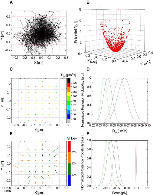
Inference of the confining potential (B), the diffusivity map (C) and the force map (E) from an experimental single CPεT receptor trajectory (A) at 21°. The average corrected inferred diffusion coefficient D_Inf is 0.08 (0.003) μm²/s and the inferred spring constant k_r is 0.75 ± 0.07 pN/μm. The value in parentheses gives the SD of the D_ij distribution. The trajectory is 1500 frames long and is confined to an area of 0.15 μm². The confinement factor u for this receptor is 0.017. The magnitude of the inferred forces is given by the length of the arrow in panel E. The color-code of the arrows shows the SD of the corresponding a-posteriori probability. (D and F) Four representative a-posteriori probabilities for the diffusivities (D) and the forces (F) found in different subdomains.

Figure 4.

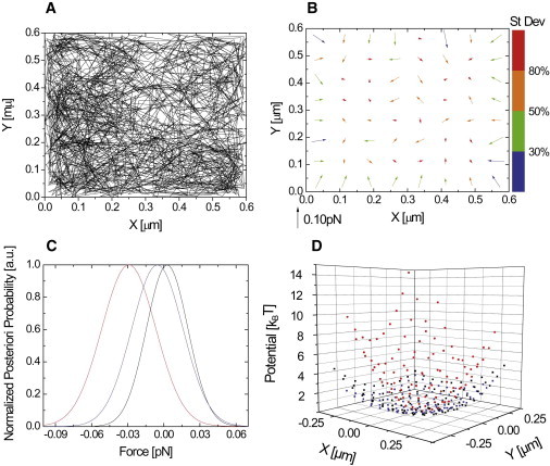
(A) Trajectory of a random two-dimensional Brownian walker, moving in a square box of length 600 nm without forces in the box. The inferred force map (B) shows small forces with random orientations. Colors are associated to error in the estimation of the forces. (C) Examples of a posteriori distributions of the forces. (D) Inferred potential (blue) compared with a typical experimental trajectory (red). The inferred potential, taking into account a static positioning noise of 25 nm (black), is also almost flat.

Depending on the experimental conditions, bias may appear and the inference may converge toward parameters shifted from their true values. To check for the presence of bias in the inferred parameters, we generated numerical trajectories for the same range of conditions as the experimental ones. Then the inference was run and the inferred values were compared to the input values. This comparison shows that systematic bias, analytically correctable, may be present in certain conditions. In the subsection Performance of the Technique (below), we show how this bias was corrected.

The inference algorithms were run on a personal computer (dual-core 3 GHz, 2 GB RAM) using C language. The inference of the force and potential map of a single trajectory with 1000 points requires, on average, a few tens of seconds to converge.

Model

The single-molecule motion is modeled by the overdamped Langevin equation,

$$\frac{d\mathbf{r}}{dt}=-\frac{\nabla V\left(\mathbf{r}\right)}{\gamma \left(\mathbf{r}\right)}+\sqrt{2D\left(\mathbf{r}\right)}\xi \left(t\right),$$ (4)

with γ(r)the spatially varying friction coefficient, D(r) the spatially varying diffusion coefficient, V(r) the potential acting on the biomolecule, and ξ(t) the rapidly varying zero-average Gaussian noise. The fluctuation-dissipation theorem gives D(r) = k_BT/γ(r) (39). With respect to the equation of motion that leads to the usual model for the MSD fit of confined trajectories (6), we introduced an additional term for an arbitrary potential (24). In contrast, in the usual model for MSD analysis of confined motion, the potential is assumed to have a square shape, i.e., no forces inside the domain, a major assumption. By allowing this potential to take an arbitrary form, this to our knowledge new method makes far fewer assumptions on the motion of the biomolecule and is thus much more versatile.

The associated Fokker-Planck equation, which governs the evolution of the transition probability over time, is given in Eq. 5 (39). Here, F(r) = −▿V(r),

$${\partial }_{t}P\left(\mathbf{r},t|{\mathbf{r}}_1,t_1\right)=-\nabla ·\left[-\frac{\nabla V\left(\mathbf{r}\right)}{\gamma \left(\mathbf{r}\right)}P\left(\mathbf{r},t|{\mathbf{r}}_1,t_1\right)-\nabla \left(D\left(\mathbf{r}\right)P\left(\mathbf{r},t|{\mathbf{r}}_1,t_1\right)\right)\right],$$ (5)

where P(r,t|r₁,t₁) is the probability of going from (r₁,t₁) to (r,t). This equation has no general solution for an arbitrary potential and a spatially varying diffusion coefficient. We therefore divide the confinement domain into subdomains using a mesh grid and the points of the trajectory are attributed to their respective grid subdomains. Within each subdomain, we consider that the potential gradient and the diffusion coefficient are constant. To avoid undersampling, the size of the mesh should be chosen so that, on average, adjacent space-time points (r_n, t_n and r_n+1, t_n+1) fall within the same or direct neighboring subdomains. This assumption enables us to solve Eq. 5, for a constant F_ij and D_ij per subdomain (i, j). This, however, does not mean that they are constant over the entire trajectory. Each subdomain is free to have a different F_ij and D_ij, which is an approximation to inferring an arbitrary potential. The assumption leads to the expression of the transition probability,

$$P\left(\left({\mathbf{r}}_2,t_2|{\mathbf{r}}_1,t_1\right)|{\mathbf{F}}_{ij},D_{ij}\right)=\frac{e^{-\frac{{\left({\mathbf{r}}_2-{\mathbf{r}}_1-{\mathbf{F}}_{ij}\left(t_2-t_1\right)/{\gamma }_{ij}\right)}^2}{4\left(D_{ij}+{\sigma }^2/\left(t_2-t_1\right)\right)\left(t_2-t_1\right)}}}{4\pi \left(D_{ij}+{\sigma }^2/\left(t_2-t_1\right)\right)\left(t_2-t_1\right)},$$ (6)

with σ the amplitude of the positioning noise (see Section S3 in the Supporting Material). This expression is the probability of going from one space-time coordinate (r₁, t₁) to the next (r₂, t₂) for a diffusivity D_ij and a force F_ij with a positioning noise σ. The overall probability of a trajectory T consisting of N space-time points (r_n, t_n) due to a certain set of variables is then computed by multiplying all the probabilities of the individual subdomains P(T|D_ij,F_ij) according to Eq. 7. The probabilities in the individual subdomains P(T|D_ij,F_ij) are computed in turn for all individual points in the data set that fall within a subdomain with Eq. 8, where μ is the index of the point in the trajectory that falls within a certain subdomain S_ij. This gives the likelihood function of

$$P\left(T|D,\mathbf{F}\right)=\prod _{i,j=1}^{i_{max},j_{max}}P\left(T|D_{ij},{\mathbf{F}}_{ij}\right),$$ (7)

$$P\left(T|D_{ij},{\mathbf{F}}_{ij}\right)=\prod _{\mu :r_{\mu }\in S_{ij}}P\left(\left({\mathbf{r}}_{\mu +1},t_{\mu +1}|{\mathbf{r}}_{\mu },t_{\mu }\right)|D_{ij},{\mathbf{F}}_{ij}\right).$$ (8)

Now that the likelihood is known, we may apply Bayes' rule,

$$P\left(Q|T\right)=\frac{P\left(T|Q\right)P_0\left(Q\right)}{P_0\left(T\right)},$$ (9)

where P(Q|T) is the posterior or a-posteriori probability of the parameters, i.e., the probability that the parameters Q take on a specific value given the recording of the trajectory T. Here, P(T|Q) is the likelihood of the trajectory, i.e., the probability of recording the trajectory T given a specific value Q of the parameters, P₀(Q) is the prior probability of the parameters, and P₀(T) is a normalization constant called the “evidence of the model” (37,38). Without prior knowledge on the parameters, the prior probability P₀(Q) is supposed to be constant over a broad range of possible values. The process is visualized schematically in Fig. 1.

Figure 1.

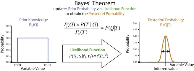
Schematic representation of the inference approach. Bayes' rule states that the a posteriori distribution P(T|Q) is equal to the product of the likelihood P(T|Q) by the prior distribution P₀(Q) divided by the evidence P₀(T). The likelihood is equal to the product of the transition probabilities P(r₂,t₂|r₁,t₁) for the complete trajectory. The peak of the a posteriori probability P(T|Q) yields the most likely value for the variable Q and its width represents the uncertainty of this inferred value.

The parameter value that yields the maximum of the a-posteriori probability is the inferred value for the parameter. The SD of the distribution yields the uncertainty on the inferred value. The optimization of the parameters maximizing the a-posteriori probability is performed first with a quasi-Newtonian optimization using the Broyden-Fletcher-Goldfarb-Shanno algorithm (35). Then, Monte Carlo sampling of the a-posteriori probability yields the SD of the parameters (35). Numerical trajectories are used to analyze the quality of the inference in Results and Discussion.

The model presented above is valid for the general case of a confined trajectory. In the following, we introduce simplifications valid for our experimental trajectories to be able to compare the inferred parameters more easily.

The confinement domain is divided into subdomains using a grid and the points of the trajectory are attributed to their respective grid subdomains. In each subdomain, we make the approximation that the potential gradient is constant so that Eq. 6 is applicable. The choice of grid subdomains depends on the type of trajectory, and should be optimized for each experimental case so that each subdomain contains a sufficient number of data points to allow obtaining meaningful inferred values for that subdomain. In particular, it is important that the grid choice is such that adjacent data points in time fall most frequently in the same or adjacent subdomains. A reasonable size for the mesh size can be obtained by first calculating the mean displacement of the particle per frame and multiplying it by 1.5. Note that nothing imposes a regular mesh, yet simulations have to confirm that irregularities do not generate local or global bias.

Experimental trajectories were analyzed with no assumptions on the diffusivity, i.e., varying diffusivities inside the domain. When the diffusivity variations inside the confinement domain are weak, an average diffusion coefficient D_Inf can be evaluated globally for the trajectory

$$\left(D_{Inf}=\frac{1}{n^2}{\sum }_{i,j}{D}_{i,j}\right),$$

where n² is the number of mesh squares. Note that, depending on experimental conditions, the inference performed with a unique, constant diffusivity and the one performed with diffusivities varying within the mesh to extract an average diffusivity, may converge toward different values. This is a consequence of the nonlinear optimization process.

For the inference of forces, two methods were applied. The first method is used to extract the force maps and the forces are optimized independently in each subdomain. Overall, this method has to optimize n² × 3 independent variables for the forces and diffusion coefficients and, concerning the forces, is the approach used in Masson et al. (24). Note that, because each mesh square is independent of the other, optimization is performed on groups of variables (D_Inf, F_ij) that are fast to compute and which converge toward meaningful values when >25 points are present in the mesh square.

For the second method, instead of inferring independent forces in a subdomain grid dividing-up the confining zone, we directly infer the parameters of a confining potential. The inference procedure optimizes the parameters of the potential, which governs the forces in each subdomain i,j via F_ij = −▿V(r_ij). The resulting forces are, however, still evaluated in each subdomain during the optimization operation and are used to calculate the a-posteriori probability. We use the polynomial potential

$$V\left(x,y\right)={\sum }_{l+m\le C}{\alpha }_k{x}^l{y}^m,$$

where k = [(1 + m)(l + m + 1)]/2 and C is the order of the polynomial. This method is used to obtain a map of the potential. In some cases, the potential can be projected on a parabolic basis and the corresponding spring constant extracted.

In most cases, confining potentials are well described by potentials of order ranging from 2 or 8. The optimal order of the polynomials can be determined by comparing the evidence of the a-posteriori obtained with polynomials of different orders (37,38). Yet, the fast convergence of the inference scheme allows us to directly check that the potential does not evolve any longer with rising order of the polynomials and that the error on the coefficients does not decrease. When the potential can be approximated by a parabolic shape, optimization is performed on n² + 5 parameters with n² the number of mesh squares. Furthermore, the radial spring constant k_r can be evaluated by allowing the comparison of different trajectories with a single variable (see Results and Discussion).

Results and Discussion

The force, potential, and diffusivity map

A single-molecule trajectory of a nanoparticle-labeled C. perfringens ε-toxin (CPεT) receptor is displayed in Fig. 2 A. A map of the inferred forces that act on the receptor within its confining domain is shown in Fig. 2 E. The forces vary in direction and magnitude, typically ranging from 0 to 0.28 pN. The diffusivity map is displayed in Fig. 2 C. The diffusivity variations within the domain are on the same order as the widths of the a posteriori probabilities for the diffusivities (Fig. 2 D and see Fig. S1 in the Supporting Material). This justifies the use of a global, constant diffusion coefficient in the accompanying article (29).

We have shown that experimental trajectories of CPεT receptors can be accurately analyzed by a second-order polynomial (29). The inferred confining potential of the CPεT receptor is shown in Fig. 2 B. Three more receptor trajectories and inferred confining potentials are shown in Fig. S1. The radial spring constant k_r can be calculated from the second-order potential by $k_r=\sqrt{k_X^2+k_Y^2},$ with k_X and k_Y the eigenvalues of the spring constant matrix [k_xx, k_xy; k_xy, k_yy]. The linear terms are negligible for all the experimental trajectories.

Performance of the technique

In the case of confined diffusion in a flat potential with infinite barriers at the domain boundaries, it was shown that the inference method reaches the best performances theoretically achievable (25). Here, we investigate with simulations the inference scheme when a spatially varying potential V(r) acts on the single molecule.

This section analyzes the performance with respect to the dimensionless confinement factor u. This factor relates the square displacement covered by the diffusing molecule during the acquisition time Δt to the total area of the confining domain:

$$u=\frac{D\Delta t}{\pi {\left(R_{.95}\right)}^2}.$$ (10)

As in all single-molecule experiments, the acquisition time Δt and the related experimental parameters, like excitation intensity and wavelength, should be chosen in such a way that u = 1.

Note that the vast parameter space, i.e., all possible confining potentials, all possible diffusivity fields, prevents us from discussing all possible cases. We will therefore focus on simple cases that emphasize the possibilities of the method. As shown in Voisinne et al. (25) for the case without a potential, the accessible information decreases exponentially with the confinement factor u.

For a large set of values for u, the inferred forces were shown to converge to the input values of numerical trajectories (24). As the confinement factor u rises, bias can emerge for some of the parameters. An example of bias is exposed here for a simplified case. Numerical trajectories with a confining harmonic potential and constant diffusivity were generated. In this specific case, for u > 0.01, the inferred D and k_r values start deviating from the numerical input values. Normalized values of inferred D and k_r as a function of u are shown in blue in Fig. 3, A and B, respectively. The plot shows the summary of 1650 trajectories, with an input diffusion coefficient of 0.075 μm²/s, 1000 data points, and an acquisition time of 51.3 ms to match experimental conditions. The confinement factor u was adjusted by varying the input k_r from 0.002 to 0.64 pN/μm. The results show that we are underestimating D and overestimating k_r. This bias is analytically deterministic and is the consequence of the constraints in the nonlinear optimization that acts on both the diffusivity and the spring constant. Therefore, the bias can be compensated for by correcting the inferred values (see Fig. 3) with the functions

$$\Delta D=Au,$$ (11)

$$\Delta k_r=B{u}^2,$$ (12)

with, in our case, A = 21.4 ± 0.2, B = −570 ± 15. The terms ΔD and Δk_r indicate the deviation of the variables D and k_r from the real (input) values, respectively, and the terms A and B are fit-parameters. The corrected inferred parameters are shown in red in Fig. 3, A and B, for D and k_r, respectively. We have studied the behavior of the parameters A and B with respect to the length N of the trajectory, the diffusion coefficient of the receptor, and the choice of the mesh in Fig. S2, Fig. S3, and Fig. S4, respectively. The correction parameters remain valid for $u<0.02$ for trajectories longer than 400 points, for diffusion coefficients ranging from 0.075 to 0.2 μm²/s, and for 6 × 6 to 10x10 mesh subdomains. For different experimental conditions or a different optimization process, the bias should be evaluated again as discussed above by using numerical trajectories. We emphasize that, the bias being systematic, and depending upon the accessible parameters only, it can be automatically corrected.

Figure 3.

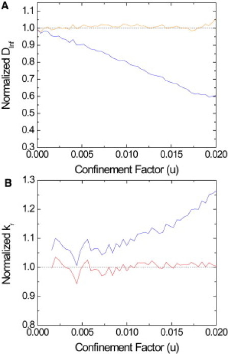
Values of inferred parameters normalized with the input values used for the numerical trajectories without (blue) and with (red) the correction of Eqs. 11 and 12 for the diffusion coefficient (A) and the calculated radial spring constant k_r (B). (Dotted black line) No-bias line. After the correction operation, we obtain results without bias.

Detection of the forces

The advantage of the inference technique is that it is not limited to extracting the diffusivity field D(r), but also extracts the confining potential V(r).

An important question is: Does the scheme tend to always detect forces even when no forces are present? We show in the following that the answer is negative.

To demonstrate that our scheme indeed finds zero forces when no forces are present, we generate numerical trajectories confined in a square box without a potential. Fig. 4 A shows an example of such a trajectory generated for a random two-dimensional Brownian walker with a diffusion coefficient of 0.075 μm²/s confined to a square box of 600 nm × 600 nm, values close to the experimental ones. The length of the trajectory is 1500 frames and the acquisition time is 51.3 ms. Fig. 4 shows the results of the inference technique plotted in the same manner as the results inferred from the experimental data in Fig. 2.

Within the confining box, the inferred force map in Fig. 4 B shows forces that are small with respect to inferred forces from experimental trajectories. Furthermore, the inferred forces have a random orientation. These forces are characterized by a large error bar, as can be seen from the color code in Fig. 4 B and the a posteriori probability plots in Fig. 4 C. The a posteriori probability distributions for the forces in the domain are very broad and always include zero force. Forces at the boundaries point toward the center of the domain and are higher. They represent the force exerted by the boundary on the Brownian walker, when it is reflected. Even restricting ourselves to a potential described by a second-order polynomial, the inferred potential in Fig. 4 D (blue) is almost flat with respect to the potential inferred from experimental data (red). When the influence of positioning noise is added to simulated trajectories, the resulting potential is still flat (black in Fig. 4 D). The spring value we find for the second-order potential, k_r = 0.12 ± 0.02 pN/μm, is well inferior to the experimental spring values. We point out that the use of a second-order polynomial for the no-force case is motivated by the comparison with experimental results. Indeed, higher-order polynomials lead to a much flatter potential with rising values only near the limits of the box. While Fig. 4 illustrates the results for a particular set of experimental parameters, Section S4 in the Supporting Material explores the value of this lower limit, restricted to a second-order polynomial, as a function of domain size and trajectory length. All the spring constants derived from experimental trajectories lie well above this lower limit, valid for a second-order polynomial analysis (see Fig. S6).

Thus, the inference scheme distinguishes between the case with no forces and real forces within our confinement domains. This in turn means that, if inference from experimental data shows forces within the domain with narrow a posteriori probabilities excluding zero as in Fig. 2 F, these forces are real and not model-induced artifacts.

Inference versus MSD

The inference technique outperforms MSD analysis in the case of a square box with no forces inside the domain, as was shown in Voisinne et al. (25). We here consider the case of confinement due to a potential. The motion of the receptor is modeled by the overdamped Langevin equation of motion (Eq. 4). This equation is much less restrictive in terms of assumptions than the usual MSD analysis (6), where the receptor is assumed to move in a Brownian fashion in a box. Obviously, the standard MSD analysis cannot find forces within the domain, simply because it starts with the assumption that there are none. In addition, this will lead to a difference in performance of the two methods in the case of a Brownian walker, which is constrained by an attractive potential as shown in Fig. 5.

Figure 5.

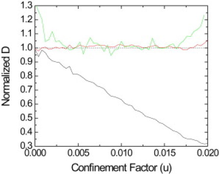
D_Inf, D_MSD, and D^′_MSD normalized with the input values for numerical trajectories confined by a spring potential. (Black curve) D_MSD obtained by fitting the first three points of the MSD data by a straight line. (Green curve) D^′_MSD, obtained by fitting the MSD plot with Eq. 2. (Red curve) Absence of bias for the corrected inferred diffusion coefficients.

It is possible to include specific shapes of potentials (mostly springlike potentials) into a modified form of the MSD. This, however, requires an a-priori knowledge of the potential form. The inference approach, in contrast, can extract the coefficients of an arbitrary polynomial potential. Furthermore, the variability of the diffusion inside the confinement domain cannot be included in the MSD analysis. We also emphasize that, if the diffusivity varies inside the domain, MSD analysis would lead to a unique value that would nontrivially depend on the diffusivity statistics in the domain. The inference approach would be able to address this diffusivity field.

We use 1650 simulated trajectories with 1000 points and an input diffusion coefficient of 0.075 μm²/s. The range of u is controlled by increasing the input spring constant of the potential V(r) = 1/2k_rr² that confines the Brownian walker. The simulation takes 1000 substeps between adjacent frames separated by 51.3 ms. The substeps are not averaged and no positioning noise is added. This analysis simply evaluates the performance of the methods on trajectories that are not obscured by noise to show how they differ on a fundamental level. Fig. 5 compares the results from both techniques for the same trajectories: the deviation of D_Inf obtained with the inference technique and corrected as discussed in Performance of the Technique is given in red, and the deviation of D_MSD and D^′_MSD are shown in black and green, respectively.

Both techniques work equally well for the extremely low or zero confinement limit and a constant diffusivity everywhere inside the domain. The SD of both techniques converges to the limit predicted by the Fisher Information and decreases with the square root of the number of data points N in the trajectory. However, as confinement becomes stronger, D_MSD shows a bias. This bias in D_MSD is due to the increase of the potential's impact on the trajectory. As forces play a larger role in the motion of the receptor, fitting the first three MSD data points with a straight line to extract the Brownian diffusion coefficient is no longer valid. D^′_MSD performs better than D_MSD but, obviously, cannot give any information about the potential. D_Inf outperforms both D_MSD and D^′_MSD.

Inference versus residence time analysis

The residence time or inversion-of-fraction technique is based on Boltzmann statistics and provides an alternative means to determine the confining potential, which is often used in the field of optical tweezers (40). The underlying assumption is that the probability of visiting a spot in an arbitrary potential is governed by Boltzmann statistics and given by the following equation:

$$N_{ij\in n}=N_0{e}^{\frac{-V_{ij}}{k_{\text{B}}T}}.$$ (13)

Here, the number of times that a subdomain ij is visited in a n × n grid, N_ij∈n, depends on the potential V_ij and the temperature T. N₀ is the number of visits to the most visited subdomain. The resulting potential in that grid subdomain can then be determined via the expression

$$V_{ij}=-k_{\text{B}}Tln\left(\frac{N_{ij}}{N_0}\right).$$ (14)

Fig. 6 shows a comparison between the potentials extracted with this residence-time technique and with the inference technique for 60,000 numerical trajectories of 500 points with an input diffusion coefficient 0.075 μm²/s and varying input spring potential. The deviation from the input potential is computed by summing up the square difference between the obtained potential and the input potential values in each subdomain. For the inference technique, we used a second-order polynomial potential (red line). For the residence-time technique, the potential was extracted either by computing independently the V_ij in Eq. 14 for each subdomain ij (arbitrary potential, black line) or by fitting the data with a spring potential (blue line). Inference outperforms both of the residence-time approaches. As expected, when the number of points in the trajectory is reduced, all techniques show a greater deviation from the input potential (data not shown).

Figure 6.

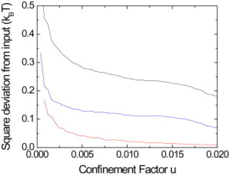
Square deviation from the input spring potential of confining potentials extracted by the inference (after correction with Eq. 12) and residence-time techniques for numerical trajectories. The deviation is shown for the residence time technique with an arbitrary potential (black), or for a fit with a spring potential (blue), and for the inference method with a second-order potential (red). The inference technique extracts a potential that is closer to the input spring potential.

The residence -time technique tends to overestimate the potential in regions that were visited less frequently and to underestimate it in the regions visited more frequently. This is the consequence of the equilibrium assumption underlying the residence time analysis. Yet, experimentally, statistical equilibrium is almost never reached. Overall, the inference technique is a valuable tool to evaluate the confining potential of a biomolecule and outperforms the residence-time technique.

Conclusion

The technique for inferring parameters from single-molecule trajectories, based on the Langevin equation of motion and using Bayes' theorem, produces highly accurate results. An extra term that allows the confining potential to take an arbitrary form makes this model less constricting than standard models in terms of assumptions. We have shown, in the case of toxin receptors confined in cell membrane microdomains, how the introduced inference method can be used on experimental single-molecule trajectories to extract the forces acting on a molecule and the confining potential. It is further possible to obtain a direct measurement of the uncertainty on the inferred values via the width of the a-posteriori probability.

Furthermore, we showed that the inference technique yields more information for a molecule in an arbitrary confining potential than the typical MSD analysis of such cases, because it uses more of the information stored in the trajectories and is less restrictive in terms of the initial assumptions. Note that the Fisher information in the presence of a potential cannot be calculated due to the size of the parameter space. Therefore, optimality of the scheme can only be tested numerically on restricted sets of parameters. Furthermore, through extensive simulations, we can quantify the efficiency, the convergence rate, and the presence of bias of the inference schemes for parameters corresponding to our experiments. With respect to the shape of the confining potential, we showed that the inference technique outperforms methods based on Boltzmann statistics. This is not surprising because the equilibrium case implicit in Boltzmann statistics is typically not reached in short single-molecule trajectories.

We also showed that the diffusion coefficient can be inferred locally instead of globally. It is also possible to test for time variations of the diffusion coefficient by analyzing sliding time-windows of the trajectory. Note, however, that, in both cases of time and space variations of the diffusion coefficient, evaluation of the diffusion coefficient in subdomains or for specific time-windows leads to reduction in the number of data points and, therefore, in the amount of information available and in the precision of the results.

The determination of the confinement potential has important implications for understanding the cell membrane organization (see Türkcan et al. (29)). As dictated by the Fisher information, the larger the number of data points in the trajectory, the more precise the extracted information (25). Extraction of the confining potential from very short trajectories will probably be meaningless, unless multiple trajectories explore the same domain. Long trajectories, however, such as those obtained with nonblinking rare-earth-doped nanoparticles, provide sufficient information to yield accurate results (29). Furthermore, different short trajectories can be included in a unique inference scheme to extract diffusivity and potential fields (J.-B. Masson, P. Dionne, M. Renner, A. Triller, and M. Dahan, unpublished).

The confinement of the CPεT and CSαT receptors observed in the experimental trajectories can be attributed to lipid rafts (29). Biochemical experiments show that lowering the level of cholesterol content in the membrane decreases confinement, while actin depolymerization has no influence on the confinement. This leads us to speculate that hydrophobic interactions between the receptor and its surrounding molecular environment create forces in the confining domain.

It is important to note that the inference technique can be applied to other cases of motion, where the receptor is not confined (J.-B. Masson, P. Dionne, M. Renner, A. Triller, and M. Dahan, unpublished). Furthermore, the scheme could be extended to deal with motions modeled by the overdamped generalized Langevin equation such as

$${\int }_0^{t}dsK\left(t-s\right)\frac{d\mathbf{r}}{dt}\left(s\right)=-\nabla V\left(\mathbf{r}\right)+\xi \left(t\right).$$

Obviously, in all these cases it is important to check the validity of the inferred values using numerical trajectories with the same characteristics as the experimental ones. Furthermore, terms can be added that directly model experimental parameters, such as the localization precision and the response of the detector.

References

- 1.Saxton M.J., Jacobson K. Single-particle tracking: applications to membrane dynamics. Annu. Rev. Biophys. Biomol. Struct. 1997;26:373–399. doi: 10.1146/annurev.biophys.26.1.373. [DOI] [PubMed] [Google Scholar]
- 2.Lord S.J., Lee H.L., Moerner W.E. Single-molecule spectroscopy and imaging of biomolecules in living cells. Anal. Chem. 2010;82:2192–2203. doi: 10.1021/ac9024889. [DOI] [PMC free article] [PubMed] [Google Scholar]
- 3.Barak L.S., Webb W.W. Diffusion of low density lipoprotein-receptor complex on human fibroblasts. J. Cell Biol. 1982;95:846–852. doi: 10.1083/jcb.95.3.846. [DOI] [PMC free article] [PubMed] [Google Scholar]
- 4.Sheetz M.P., Turney S., Elson E.L. Nanometer-level analysis demonstrates that lipid flow does not drive membrane glycoprotein movements. Nature. 1989;340:284–288. doi: 10.1038/340284a0. [DOI] [PubMed] [Google Scholar]
- 5.Fourier J., Freeman A. Cambridge University Press; New York: 2009. The Analytical Theory of Heat. [Google Scholar]
- 6.Kusumi A., Sako Y., Yamamoto M. Confined lateral diffusion of membrane receptors as studied by single particle tracking (nanovid microscopy). Effects of calcium-induced differentiation in cultured epithelial cells. Biophys. J. 1993;65:2021–2040. doi: 10.1016/S0006-3495(93)81253-0. [DOI] [PMC free article] [PubMed] [Google Scholar]
- 7.Lommerse P.H., Blab G.A., Schmidt T. Single-molecule imaging of the H-Ras membrane-anchor reveals domains in the cytoplasmic leaflet of the cell membrane. Biophys. J. 2004;86:609–616. doi: 10.1016/S0006-3495(04)74139-9. [DOI] [PMC free article] [PubMed] [Google Scholar]
- 8.Pinaud F., Michalet X., Weiss S. Dynamic partitioning of a glycosyl-phosphatidylinositol-anchored protein in glycosphingolipid-rich microdomains imaged by single-quantum dot tracking. Traffic. 2009;10:691–712. doi: 10.1111/j.1600-0854.2009.00902.x. [DOI] [PMC free article] [PubMed] [Google Scholar]
- 9.Schütz G.J., Schindler H., Schmidt T. Single-molecule microscopy on model membranes reveals anomalous diffusion. Biophys. J. 1997;73:1073–1080. doi: 10.1016/S0006-3495(97)78139-6. [DOI] [PMC free article] [PubMed] [Google Scholar]
- 10.Deverall M.A., Gindl E., Naumann C.A. Membrane lateral mobility obstructed by polymer-tethered lipids studied at the single molecule level. Biophys. J. 2005;88:1875–1886. doi: 10.1529/biophysj.104.050559. [DOI] [PMC free article] [PubMed] [Google Scholar]
- 11.Hebert B., Costantino S., Wiseman P.W. Spatiotemporal image correlation spectroscopy (STICS) theory, verification, and application to protein velocity mapping in living CHO cells. Biophys. J. 2005;88:3601–3614. doi: 10.1529/biophysj.104.054874. [DOI] [PMC free article] [PubMed] [Google Scholar]
- 12.Coscoy S., Huguet E., Amblard F. Statistical analysis of sets of random walks: how to resolve their generating mechanism. Bull. Math. Biol. 2007;69:2467–2492. doi: 10.1007/s11538-007-9227-8. [DOI] [PubMed] [Google Scholar]
- 13.Condamin S., Tejedor V., Klafter J. Probing microscopic origins of confined subdiffusion by first-passage observables. Proc. Nat. Acad. Sci. USA. 2008;105:5675–5680. doi: 10.1073/pnas.0712158105. [DOI] [PMC free article] [PubMed] [Google Scholar]
- 14.Jin S., Haggie P.M., Verkman A.S. Single-particle tracking of membrane protein diffusion in a potential: simulation, detection, and application to confined diffusion of CFTR Cl− channels. Biophys. J. 2007;93:1079–1088. doi: 10.1529/biophysj.106.102244. [DOI] [PMC free article] [PubMed] [Google Scholar]
- 15.Ryan T.A., Myers J., Webb W.W. Molecular crowding on the cell surface. Science. 1988;239:61–64. doi: 10.1126/science.2962287. [DOI] [PubMed] [Google Scholar]
- 16.Dix J.A., Verkman A.S. Crowding effects on diffusion in solutions and cells. Annu. Rev. Biophys. 2008;37:247–263. doi: 10.1146/annurev.biophys.37.032807.125824. [DOI] [PubMed] [Google Scholar]
- 17.Sieber J.J., Willig K.I., Lang T. The SNARE motif is essential for the formation of syntaxin clusters in the plasma membrane. Biophys. J. 2006;90:2843–2851. doi: 10.1529/biophysj.105.079574. [DOI] [PMC free article] [PubMed] [Google Scholar]
- 18.Douglass A.D., Vale R.D. Single-molecule microscopy reveals plasma membrane microdomains created by protein-protein networks that exclude or trap signaling molecules in T cells. Cell. 2005;121:937–950. doi: 10.1016/j.cell.2005.04.009. [DOI] [PMC free article] [PubMed] [Google Scholar]
- 19.Sheetz M.P. Glycoprotein motility and dynamic domains in fluid plasma membranes. Annu. Rev. Biophys. Biomol. Struct. 1993;22:417–431. doi: 10.1146/annurev.bb.22.060193.002221. [DOI] [PubMed] [Google Scholar]
- 20.Kusumi A., Ike H., Fujiwara T. Single-molecule tracking of membrane molecules: plasma membrane compartmentalization and dynamic assembly of raft-philic signaling molecules. Semin. Immunol. 2005;17:3–21. doi: 10.1016/j.smim.2004.09.004. [DOI] [PubMed] [Google Scholar]
- 21.Peters I.M., van Kooyk Y., Greve J. 3D single-particle tracking and optical trap measurements on adhesion proteins. Cytometry. 1999;36:189–194. doi: 10.1002/(sici)1097-0320(19990701)36:3<189::aid-cyto7>3.3.co;2-v. [DOI] [PubMed] [Google Scholar]
- 22.Varma R., Mayor S. GPI-anchored proteins are organized in submicron domains at the cell surface. Nature. 1998;394:798–801. doi: 10.1038/29563. [DOI] [PubMed] [Google Scholar]
- 23.Lingwood D., Simons K. Lipid rafts as a membrane-organizing principle. Science. 2010;327:46–50. doi: 10.1126/science.1174621. [DOI] [PubMed] [Google Scholar]
- 24.Masson J.-B., Casanova D., Alexandrou A. Inferring maps of forces inside cell membrane microdomains. Phys. Rev. Lett. 2009;102:48103. doi: 10.1103/PhysRevLett.102.048103. [DOI] [PubMed] [Google Scholar]
- 25.Voisinne G., Alexandrou A., Masson J.-B. Quantifying biomolecule diffusivity using an optimal Bayesian method. Biophys. J. 2010;98:596–605. doi: 10.1016/j.bpj.2009.10.051. [DOI] [PMC free article] [PubMed] [Google Scholar]
- 26.Tilley S.J., Saibil H.R. The mechanism of pore formation by bacterial toxins. Curr. Opin. Struct. Biol. 2006;16:230–236. doi: 10.1016/j.sbi.2006.03.008. [DOI] [PubMed] [Google Scholar]
- 27.Gordon V.M., Nelson K.L., Leppla S.H. Clostridium septicumα-toxin uses glycosylphosphatidylinositol-anchored protein receptors. J. Biol. Chem. 1999;274:27274–27280. doi: 10.1074/jbc.274.38.27274. [DOI] [PubMed] [Google Scholar]
- 28.Cole A.R., Gibert M., Basak A.K. Clostridium perfringensε-toxin shows structural similarity to the pore-forming toxin aerolysin. Nat. Struct. Mol. Biol. 2004;11:797–798. doi: 10.1038/nsmb804. [DOI] [PubMed] [Google Scholar]
- 29.Türkcan S., Masson J.-B., Alexandrou A. Observing the confinement potential of bacterial pore-forming toxin receptors inside rafts with nonblinking Eu3+-doped oxide nanoparticles. Biophys. J. 2012;102:2299–2308. doi: 10.1016/j.bpj.2012.03.072. [DOI] [PMC free article] [PubMed] [Google Scholar]
- 30.Casanova D., Giaume D., Alexandrou A. Counting the number of proteins coupled to single nanoparticles. J. Am. Chem. Soc. 2007;129:12592–12593. doi: 10.1021/ja0731975. [DOI] [PubMed] [Google Scholar]
- 31.Qian H., Sheetz M.P., Elson E.L. Single particle tracking. Analysis of diffusion and flow in two-dimensional systems. Biophys. J. 1991;60:910–921. doi: 10.1016/S0006-3495(91)82125-7. [DOI] [PMC free article] [PubMed] [Google Scholar]
- 32.Destainville N., Salomé L. Quantification and correction of systematic errors due to detector time-averaging in single-molecule tracking experiments. Biophys. J. 2006;90:L17–L19. doi: 10.1529/biophysj.105.075176. [DOI] [PMC free article] [PubMed] [Google Scholar]
- 33.Savin T., Doyle P.S. Role of a finite exposure time on measuring an elastic modulus using microrheology. Phys. Rev. E Stat. Nonlin. Soft Matter Phys. 2005;71:041106. doi: 10.1103/PhysRevE.71.041106. [DOI] [PubMed] [Google Scholar]
- 34.Michalet X. Mean square displacement analysis of single-particle trajectories with localization error: Brownian motion in an isotropic medium. Phys. Rev. E Stat. Nonlin. Soft Matter Phys. 2010;82:041914. doi: 10.1103/PhysRevE.82.041914. [DOI] [PMC free article] [PubMed] [Google Scholar]
- 35.Press W., Vetterling W., Flannery B. Cambridge University Press; New York: 2001. Numerical Recipes in C++: The Art of Scientific Computing. [Google Scholar]
- 36.Krauth W. Oxford University Press; New York: 2006. Algorithms and Computations. [Google Scholar]
- 37.MacKay D. Cambridge University Press; Cambridge, UK: 2003. Information Theory, Inference, and Learning Algorithms. [Google Scholar]
- 38.Von Toussaint U. Bayesian inference in physics. Rev. Mod. Phys. 2011;83:943–999. [Google Scholar]
- 39.Risken H. Springer-Verlag, Berlin, Heidelberg; New York: 1996. The Fokker-Planck Equation: Methods of Solution and Applications. [Google Scholar]
- 40.Florin E., Pralle A., Hörber J. Photonic force microscope calibration by thermal noise analysis. Appl. Phys., A Mater. Sci. Process. 1998;66:75–78. [Google Scholar]
Associated Data
This section collects any data citations, data availability statements, or supplementary materials included in this article.