Theory of the energy transfer efficiency and fluorescence lifetime distribution in single-molecule FRET

Abstract

In single-molecule FRET experiments with pulsed lasers, not only the colors of the photons but also the fluorescence lifetimes can be monitored. Although these quantities appear to be random, they are modulated by conformational dynamics. In order to extract information about such dynamics, we develop the theory of the joint distribution of FRET efficiencies and fluorescence lifetimes determined from bins (or bursts) of photons. Our starting point is a rigorous formal expression for the distribution of the numbers of donor and acceptor photons and donor lifetimes in a bin that treats the influence of conformational dynamics on all timescales. This formula leads to an analytic result for a two-state system interconverting on a timescale slower than the interphoton time and to an efficient simulation algorithm for multistate dynamics. The shape of the joint distribution contains more information about conformational dynamics than the FRET efficiency histogram alone. In favorable cases, the connectivity of the underlying conformational states can be determined directly by simple inspection of the projection of the joint distribution on the efficiency-lifetime plane.

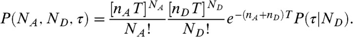
Single-molecule FRET experiments provide information about both structure and dynamics and have led to insights in a variety of biological processes including protein and RNA folding, enzyme catalysis, and protein–protein interactions (1–4). Consider a molecule with attached donor and acceptor fluorescent dyes. The donor is excited by a train of laser pulses (blue arrow in Fig. 1A). The excited donor can decay radiatively or nonradiatively or the excitation can be transferred to the acceptor. The excited acceptor can decay nonradiatively or by emitting a photon. The time between laser pulses (on the order of tens of nanoseconds) is much longer than the lifetimes of the excited states. The output of such an experiment is shown schematically in Fig. 1B. For each photon one can determine its color, arrival time, and delay time, which is the time interval between the laser pulse and the detection of the photon. For the sake of simplicity, only the delay times of the donor photons are shown, but acceptor delay times can readily be considered. The average of the delay times over the entire photon trajectory is the fluorescence lifetime of the donor in the presence of the acceptor. This experiment contains information about structure and dynamics because the photon colors and delay times depend on the rate of energy transfer. This rate in turn depends on the distance between the dyes (as distance^-6) and their relative orientation, and can fluctuate on a variety of timescales from picoseconds to seconds.

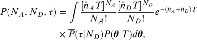
Fig. 1.

(A) The simplest kinetic scheme for FRET. A donor is excited by a laser pulse (blue arrow). The excited state can decay radiatively (green wiggly arrow) or nonradiatively (black arrow) with a combined rate k_D or the excitation can be transferred to the acceptor with rate k_ET. The acceptor can decay by emitting a photon or nonradiatively with a combined rate k_A. (B) A schematic representation (not to scale) of the sequence of donor (green) and acceptor (red) photons detected after excitation by a train of laser pulses (blue). For each donor photon, the time δt between laser pulse and the photon (delay time) is recorded. The photon sequence is divided into bins of duration T. (C) Simulated two-dimensional histogram of FRET efficiencies (E) and relative donor lifetimes (τ/τ_D, where τ_D = 1/k_D) for a three-state system. The magenta and cyan histograms are the FRET efficiency and donor lifetime histograms, respectively.

Suppose that the experimental photon trajectory is divided into time bins (see Fig. 1B). The FRET efficiency in a bin, E, is defined as the ratio of the acceptor photon counts to the total number of photons in a bin. We define the donor fluorescence lifetime in a bin, τ, as the sum of all donor delay times divided by the number of donor photons. When there are so many photons in each bin that shot noise is negligible and when conformational dynamics is so slow that transitions between conformational states are separated by many bins, then the observed E and τ trajectories directly reflect how states with the same FRET efficiency and/or fluorescence lifetime interconvert. Under less ideal circumstances, both E and τ fluctuate from bin to bin and the probability distribution of these random variables (i.e., the joint FRET efficiency-lifetime histogram) is illustrated in Fig. 1C.

The projection of this two-dimensional distribution on the E axis is the familiar FRET efficiency histogram (purple in Fig. 1C) which was the focus of our previous work (5–7) on the analysis of binned photon trajectories. However, there is additional information contained in fluorescence lifetimes (8–14) and the advantages of the simultaneous detection and analysis of both lifetimes and fluorescence intensities have been emphasized by Seidel and coworkers (4, 8, 10).

Here we extend our previous work and consider the joint FRET efficiency and fluorescence lifetime distribution. Our theory exploits the fundamentally different role played by dynamics that are slower than the interphoton time (5). With current technology, this time is longer than a microsecond. If all dynamics were faster than the time between photons, then the distribution of photons would be Poissonian. Single-molecule and ensemble experiments in this case would contain the same information. A Poisson distribution is completely determined by the mean numbers of photons detected per unit time, which are directly related to the ensemble steady-state fluorescence intensities. The distribution of delay times can be single- or multiexponential depending on whether the dynamics are faster or slower than the excited-state lifetime, just as in ensemble measurements (15). It is only when conformational changes are comparable to or slower than the interphoton time that single-molecule experiments contain more information than ensemble ones. This case of course includes heterogeneous systems when molecules do not interconvert during the timescale of the experiment, and one of the most common and useful applications of single-molecule histograms is to separate subpopulations of such molecules.

Theory

We are interested in the joint distribution P(N_A,N_D,τ) of finding N_A acceptor photons, N_D donor photons, and donor fluorescence lifetime τ in a bin of duration T. The fluorescence lifetime in a bin is defined as the average of all donor delay times in that bin, . FRET efficiency in a bin is related to the photon counts by E = N_A/(N_A + N_D).

We start by assuming that the fluctuations of the energy transfer rate are faster than the interphoton times (i.e., occur on the submicrosecond timescale). In this case, there is no correlation between consecutive photons. The statistics of the acceptor and the donor photon counts are Poissonian (5) and completely determined by the count rates n_A and n_D (i.e., the mean numbers of acceptor and donor photons per unit time, respectively). The donor delay times are also uncorrelated and have the same distribution, which we denote as . This distribution is normalized and proportional to the ensemble time-dependent donor fluorescence intensity. Thus when all dynamics are fast compared to the interphoton time, the joint distribution is

[1]

Here P(τ|N_D) is the distribution of , where the delay times δt_i are uncorrelated and distributed according to . For this distribution, the average FRET efficiency over all bins is , and the average fluorescence lifetime is (i.e., the average delay time).

Because the count rates and the average delay time all depend on the energy transfer rate (see SI Text, Fixed energy transfer rate), and are related. When all dynamics are faster than the donor lifetime, the distribution of the delay times is single-exponential. In this case, it is well known (16) that the fluorescence lifetime in the presence of acceptor and the FRET efficiency are related by

[2]

where 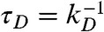is the donor lifetime in the absence of acceptor.

When the energy transfer rate fluctuates on a timescale comparable to or slower than the donor lifetime, the delay time distribution becomes multiexponential. Although there exists a general relation between the FRET efficiency and the average donor excited-state lifetime (7, 17), like Eq. 2, no such general relation exists for the donor fluorescence lifetime (which is the mean lifetime of the excited state on condition that it decays by emitting a photon; see SI Text, Influence of dynamics on lifetimes and count rates).

However, in the special case that the fluctuations of the energy transfer rate are much slower than the lifetime, it can be shown that (see SI Text, Average fluorescence lifetime, count rates and FRET efficiency when dynamics are slower than the lifetime) and are related by

[3]

where with the averaging being over all states that have different energy transfer rates k_ET. As an example, suppose that the reorientational dynamics of the dyes is very fast so that k_ET = k_D(R₀/r)⁶, where r is the interdye distance and R₀ is the Förster radius. When the interdye distance fluctuates on a timescale slower than the donor lifetime, we have 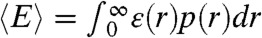, , where ε(r) = (1 + (r/R₀)⁶)^-1 and p(r) is the normalized distribution of the interdye distances.

Because the variance is always positive, the donor fluorescence lifetime is shifted toward longer values, . Thus the violation of Eq. 2 (i.e., the measured is bigger than ), is a sign of the presence of dynamics that are slow compared to the lifetime, as noted previously by Seidel and coworkers (4, 10).

Now consider fluctuations of the energy transfer rate that occur on a timescale comparable to or slower than the interphoton times. During the bin time, the molecule explores a variety of conformational states s with different count rates n_A(s), n_D(s) and delay time distributions . The conformational state index s can be discrete or continuous. The time average of the count rate in a bin, defined as , fluctuates from bin to bin. The distribution of photons in bins with the same and is uncorrelated Poissonian. The distribution of delay times in these bins is (see SI Text, Joint Distribution of Photon Counts and Fluorescence Lifetimes)

[4]

Note that the state-dependent delay time distributions, , are weighted not only by the time spent in the state, but also by the donor count rate of that state. The joint distribution of photon counts N_A and N_D and fluorescence lifetimes τ is given by (see SI Text, Joint Distribution of Photon Counts and Fluorescence Lifetimes)

[5]

where the average is over all state trajectories s(t) and 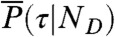is the distribution of 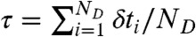with the delay times δt_i distributed according to in Eq. 4; this is one of the key results of this paper.

For a discrete model of dynamics, each conformational state s, s = 1,2,…,M, has delay time distribution and count rates n_As and n_Ds. Let θ_s be the fraction of time spent in state s during the bin time T. Thus 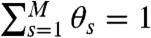, so only M - 1 θ values s are independent. The θ values fluctuate depending on which states have been visited. The time average count rates and delay time distribution (see Eq. 4) are

[6]

The joint distribution in Eq. 5 can be then written as

[7]

where θ is a vector with components θ_s, and P(θ|T) is the probability that, in a conformational trajectory of length T starting from equilibrium, the fraction of time the system spends in state s is θ_s, s = 1,2,…,M.

For a two-state system (θ₂ = 1 - θ₁), P(θ₁|T) is known analytically (18) and the resulting joint distribution is given in SI Text, Joint Distribution for a Two-State Molecule. For more than two states, it is possible to devise analytic approximations for the joint distribution along the lines of our previous work on FRET efficiency distributions (19). However, it seems easier to simulate the joint distribution using an efficient algorithm based on Eq. 7. Instead of generating trajectories photon-by-photon and then binning, we first simulate conformational trajectories of duration T using the Gillespie algorithm (20) and choose N_A, N_D, and τ from the appropriate distributions as explained in Methods.

Finally, we should point out that the expression in Eq. 5 remains valid when the definition of a “conformational state” is generalized to include any configuration of the entire system that has lifetimes and count rates that fluctuate on a timescale comparable to or slower than the mean interphoton time. For example, the count rate can fluctuate as a molecule diffuses through a confocal laser spot or because the fluorophores have several long-lived photophysical states with different emission characteristics.

Results and Discussion

We begin by considering an immobilized molecule that slowly interconverts between two states. The count rates and the average fluorescence lifetimes of the states are n_As, n_Ds, and τ_s, s = 1,2. The joint distribution P(N_A,N_D,τ) for this system can be expressed analytically. The result (see SI Text, Joint Distribution for a Two-State Molecule) is rather complicated and so it is of interest to examine the limit where the count rates are sufficiently large so that fluctuations due to the finite number of photons in a bin (shot noise) become negligible. In this case, the Poisson distributions in Eq. 7 turn into δ-functions centered on and , where θ₁ = 1 - θ₂ is the fraction of time spent in state 1. Similarly, the distribution of lifetimes, , becomes a δ-function centered on (τ₁n_D1θ₁ + τ₂n_D2θ₂)/(n_D1θ₁ + n_D2θ₂) (see Eq. 6). Thus, P(N_A,N_D,τ) becomes a product of three δ-functions weighted by P(θ₁|T) and integrated over θ₁. Consequently, the FRET efficiency-lifetime distribution is confined to a curved line where τ and E are related by (see SI Text, Two-State Dynamic Lines)

[8]

for E in the range ε₁ ≤ E ≤ ε₂, where ε_s is the FRET efficiency of state s. The distribution of points on this line is the FRET efficiency distribution in the absence of shot noise (21).

In the special case when the lifetimes and FRET efficiencies of the states are related by τ_s/τ_D = 1 - ε_s, s = 1,2, Eq. 8 simplifies. If we eliminate τ₁ and τ₂, we find

[9]

for ε₁ ≤ E ≤ ε₂. If, on the other hand, we eliminate ε₁ and ε₂ from Eq. 8, we have for τ₂ ≤ τ ≤ τ₁

[10]

This result was obtained by Kalinin et al. (10) in a different way and called the dynamic FRET equation.

Eqs. 3 and 9 have similar structure [in fact, for a two-state system, ], but their meaning is quite different. Eq. 3 describes how the average fluorescence lifetime and average FRET efficiency of a single state are related in the presence of fluctuations on a timescale longer than a few nanoseconds. Eq. 9, on the other hand, describes how the FRET efficiency-lifetime distribution behaves when two states interconvert on a timescale slower than the interphoton time.

Eqs. 8–10 describe the line that connects two states in the density plot of the joint distribution of E and τ in the absence of shot noise. In multistate systems, when the bin time is sufficiently short, only pairs of states that are directly connected by a single transition are visited. Those bins during which the molecule explores no more than two states result (because of shot noise) in a curved band of density connecting the two states in the E and τ density histogram. In this way, one can directly visualize the connectivity of the states.

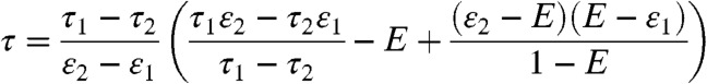
As an example, consider a three-state system with FRET efficiencies ε₁, ε₂, and ε₃ with ε₁ < ε₂ < ε₃. For simplicity, we assume that the energy transfer rate does not fluctuate on submicrosecond timescale so that the corresponding lifetimes are related to the ε values by τ_s/τ_D = 1 - ε_s, s = 1,2,3. We consider three possible kinetic schemes: (i) ε₁⇌ε₂⇌ε₃, (ii) ε₂⇌ε₁⇌ε₃, and (iii) a triangular scheme with transitions between all states, and obtain the E-τ density histogram using the algorithm described in Methods. The results for increasing bin times are shown in Fig. 2. On the top, the kinetic schemes have been redrawn so that the FRET efficiencies of the states are in increasing order. When the bin time is so short that very few transitions occur, the histograms are similar for all kinetic schemes and consist of three peaks centered on the FRET efficiencies, ε_s, and lifetimes, τ_s, of the three states (first row in Fig. 2A). Because all states obey Eq. 2, the centers of the peaks are on the diagonal. The width of the peaks is determined by shot noise. The first state is spread out more in the τ direction because the shot noise variance of τ/τ_D for state s is approximately (1 - ε_s)/(n_As + n_Ds)T. The corresponding variance in the E direction is approximately ε_s(1 - ε_s)/(n_As + n_Ds)T, so that the ratio of the two variances is ε_s. Thus the widths differ when the FRET efficiency is small.

Fig. 2.

Two-dimensional density histograms of the FRET efficiency and the ratio of the donor fluorescence lifetime in the presence and absence of acceptor (τ/τ_D), for a molecule with three interconverting states. (A) The histograms for three different connectivities of the states (columns) and increasing bin times (rows, top to bottom T = 1, 6, 30 ms). The full histogram corresponding to the center panel is shown in Fig. 1C. The FRET efficiencies of the states increase from left to right and their connectivity is shown at the top. All transitions are reversible with the same rate 0.1 ms^-1. The FRET efficiencies are ε₁ = 0.2, ε₂ = 0.5, and ε₃ = 0.8 and corresponding lifetime ratios are 0.8, 0.5, and 0.2. The histograms were simulated using the algorithm discussed in Methods with n_As + n_Ds = 100 ms^-1, s = 1,2,3. (B) The superposition of the histogram for T = 6 ms with the two-state dynamic lines (black) calculated using Eq. 9 for all pairs of directly connected states.

As the bin time increases, transitions between conformational states begin to occur. At first, only pairs of states that are nearest neighbors in the kinetic scheme are visited during the bin time. This results in an increase in density between these states (see the second row in Fig. 2A). All three density histograms look remarkably similar to the corresponding kinetic schemes shown at the top. In Fig. 2B, the two-state dynamic lines (black) calculated using Eq. 9 for each pair of directly connected states are superimposed on the histograms. For this bin time, the density histograms are just a fuzzy version of the two-state lines. At longer bin times, all three states are visited and the area bounded by the two-state lines is filled out (the third row in Fig. 2A). At very long times, the distribution collapses to a single peak centered on the equilibrium averages of the FRET efficiency and fluorescence lifetime.

Density histograms for four states with various connectivities are shown in Fig. S1. The connectivity of the states is again apparent from these density histograms, which superimpose nicely on the two-state dynamics lines.

These are of course rather idealized examples in which the FRET efficiencies of the states are well separated and all transition rates are the same. In general, although it will be not possible to determine all the connectivities visually, the FRET efficiency-lifetime histogram puts more constraints on possible models than the FRET efficiency histogram alone. The algorithm described in Methods can be used to fit kinetic models of conformational dynamics to experimental two-dimensional histograms. The adjustable parameters are the rate constants, the count rates n_As and n_Ds, and the mean and variance of the delay times, 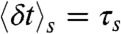and , in each state. These parameters are apparent and their values are influenced by background noise, cross-talk, direct acceptor excitation, the shape of the excitation pulse, etc. We have discussed elsewhere (7) how the fitted count rates can be simply corrected before using them to get distance information. A similar strategy can be applied to the mean and variance of the delay time distribution of each state.

Dynamics on Submicrosecond Timescale and Quenching.

In the above example, the energy transfer rate fluctuated on the millisecond timescale, which is slower than the interphoton times. What happens when there are also dynamics on the submicrosecond timescale? Such dynamics simply alters the relationship between the efficiencies and the fluorescence lifetimes from linear to the result in Eq. 3. Because , τ_s/τ_D≥1 - ε_s for state s, the peaks in Fig. 2 would be shifted away from the diagonal toward longer lifetimes (i.e., move up). The two-state dynamic lines in this case are given by the general result in Eq. 8. Thus, qualitatively, the density histograms look similar in the absence or presence of submicrosecond dynamics, except that in the latter case the peaks are shifted above the diagonal and the two-state dynamic lines adjusted accordingly (see Fig. S2 for an example).

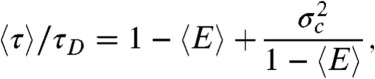
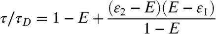
In the presence of donor quenching, the peaks can move below the diagonal (4). Quenching is a process that increases the nonradiative decay rate, thereby reducing the lifetime and the quantum yield. However, it turns out (see SI Text, Fixed energy transfer rate) that donor quenching does not affect the ratio of the donor and acceptor count rates and hence the apparent FRET efficiency. As a simple example, consider the three-state schemes in Fig. 2 and assume that states 1 and 2 have the same interdye distance but the donor in state 2 is quenched. Thus ε₁ = ε₂, but τ₂ < τ₁ = τ_D(1 - ε₁), where τ_D is the donor lifetime in the absence of both FRET and quenching. In Fig. 3, we show how the density histograms are modified when the bin time is the same as that in Fig. 2B. The two-state dynamic lines calculated from Eq. 8 superimpose as before. By moving states significantly away from the diagonal, quenching makes it easier to see the connectivities of the states.

Fig. 3.

The influence of donor quenching on the FRET efficiency and lifetime density histogram shown in Fig. 2B. The FRET efficiencies of the states are ε₁ = 0.2, ε₂ = 0.2, ε₃ = 0.8 and corresponding relative lifetimes 0.8, 0.5, and 0.2. All other parameters are the same except the total count rate in the second state is reduced because of quenching, n_A2 + n_D2 = 62.5 ms^-1.

Diffusing Molecules: Histograms by Recoloring.

When a molecule diffuses through a laser spot, a burst of photons is generated. The average duration of such bursts is a few milliseconds. The photon count rates fluctuate as the molecule traverses the confocal spot because the laser intensity is not uniform. As noted above, Eq. 5 for the joint probability distribution is exact in this case if one also averages over all paths of a molecule diffusing through the laser spot. It can be shown (see SI Text, Two-State Dynamic Lines for Diffusing Molecules) that Eq. 8 for the two-state dynamic line is also valid in the presence of translational diffusion if the ratio of donor and acceptor detection efficiencies does not depend on the molecule’s location in the laser spot. When the entire photon trajectory is divided into bins, it is possible to generalize our previous work (5) and reduce the calculation of the generating function of the joint distribution to the solution of a reaction–diffusion equation (see SI Text, Generating Function in the Presence of Diffusion and Conformational Dynamics). Although this exact formalism is mathematically elegant, it is not practical in part because the results are sensitive to the laser intensity profile of the observation volume (22). This sensitivity also limits the utility of Brownian dynamics simulations of the molecule’s trajectory through the laser spot.

In the absence of conformational changes, Antonik et al. (23) and Nir et al. (24) realized that one can circumvent the need to model translational diffusion. For a single conformation, the joint distribution of finding N_A and N_D photons in a burst can be factored into a product of the distribution of the total number of photons, which can be obtained from experiment, and a binomial distribution, which determines the color of the photons. One may expect that this factorization is also possible in the presence of conformational dynamics when (i) the total count rate n_As + n_Ds is independent of conformational state s, (ii) the apparent FRET efficiency of state s, ε_s = n_As/(n_As + n_Ds), does not depend on the location of the molecule in the laser spot, and (iii) all conformations have the same diffusion constant. However, even under these simplifying assumptions, we found that the joint distribution does not rigorously factor (6) (see SI Text, Joint Distribution for Diffusing Molecules where lifetimes are also considered). Factorization is a good approximation only when the molecule is quasi-immobilized during the observation time—i.e., it explores only a region of the laser spot where the sum of donor and acceptor count rates does not change significantly. This approximation, which is also implicitly invoked in photon distribution analysis (10, 23, 24), can be useful when bursts are preselected so that the intensity is fairly uniform and when analytic expressions are available for the conformation dependent part of the distribution. If one, however, wants to fit experimental histograms by simulating multistate models of conformational dynamics, one can avoid the quasi-immobilization approximation by using the recoloring algorithm presented below.

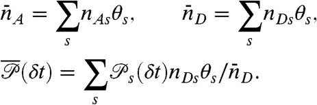
This algorithm involves recoloring the experimental photon trajectory from which the colors have been erased. It is exact for diffusing molecules when the above three conditions are met. In the absence of delay times, we have previously used a photon-by-photon recoloring scheme to validate parameters extracted from data using a maximum likelihood method (25). A more efficient burst-by-burst recoloring scheme that can be used to fit experimental FRET efficiency and lifetime histograms by varying the model parameters is shown in Fig. 4 (the step-by-step algorithm is given in Methods). For each burst or fragment of a burst selected for histogram analysis (Fig. 4B), a conformational state trajectory of length equal to the burst duration is generated. The state trajectory and the colorless experimental burst are superimposed (see Fig. 4C) and the number of photons in each state is counted. The random numbers of acceptor and donor photons are generated for each state from the appropriate binomial distribution that depends on the apparent FRET efficiency of the state and the total number of photons in that state. Finally, a random delay time is generated for each donor photon in a given state (see Fig. 4D). In this way, the total number of photons is the same as in the experimental burst, but the numbers of acceptor (donor) photons and the lifetimes, in general, differ. In the absence of lifetimes, this procedure is similar to that recently proposed by Torella et al. (26).

Fig. 4.

The burst-by-burst recoloring algorithm for data analysis. (A) Molecules diffusing through a laser spot. (B) A sequence of donor (green) and acceptor (red) photons in a burst of duration T. (C) The superposition of the photon sequence, from which the colors have been erased, with a three-state conformational trajectory. (D) Photons emitted by the same conformational state are first grouped together and then recolored using the appropriate binomial distribution (see Methods). Each donor photon in a given state is then assigned a random delay time (arrows). Finally, all photons and delay times from different states are combined.

This burst-by-burst recoloring procedure is not based on the assumption of quasi-immobilization that is implicit in all approaches that use experimentally determined distribution of the total number of photons. It circumvents the need to model diffusion by using the observed photon arrival times rather than just distribution of the total number of photons.

Concluding Remarks

We have developed the theory of joint FRET efficiency and fluorescence lifetime distributions for a single molecule that can undergo conformational changes on a variety of timescales. We found that, in favorable cases, one can establish the number and connectivity of the underlying conformational states by simply looking at the FRET efficiency-lifetime density histograms. In less favorable cases, efficient algorithms are provided that allow one to fit experimentally determined histograms to various models of conformational dynamics.

The focus of this work was on FRET but it is clear that our formalism also describes experiments in which the count rate and lifetime of a single dye fluctuates due to conformational changes (e.g., the nonradiative decay rate is modulated by quenching). Previously, we considered how two-state conformational changes influence the histogram of the number of photons of a single color in a bin (27). The corresponding joint distribution of the numbers of photons and fluorescence lifetimes is a special case of the results presented here.

Finally, we would like to point out how a complimentary method based on constructing the photon-by-photon likelihood function that we developed (25) to analyze single-molecule FRET experiments (28) can be readily extended to include lifetime information. Consider a sequence of N_ph photons detected at times t_i with colors c_i and delay times δt_i, i = 1,2,…,N_ph. We previously constructed the likelihood, L, that a discrete model of conformational dynamics describes the observed photon colors. The extension of the likelihood to include donor and acceptor delay times is

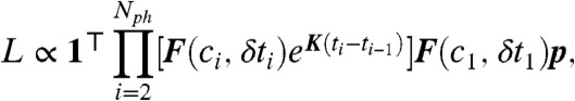[11]

where K is the rate matrix that describes transitions between states, 1^⊤ is a row vector with all elements equal to unity, p is the column vector of equilibrium populations, F(c_i,δt_i) is a diagonal matrix with the elements 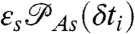if the ith photon is red (c_i = acceptor) and 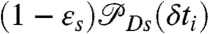if it is green (c_i = donor). Here ε_s is the apparent FRET efficiency of state s, an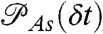d , and 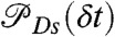are the acceptor and donor delay time distributions of state s. For diffusing molecules, this procedure, just like the recoloring algorithm described above, does not require the quasi-immobilization approximation.

Methods

FRET Efficiency-Lifetime Histograms for Immobilized Molecules.

Our algorithm to generate FRET efficiency-lifetime histograms for a model with multiple discrete states is based on the Monte-Carlo evaluation of the integrals over the fractional occupancies in Eq. 7. Each state s has photon count rates n_As and n_Ds and donor delay time distribution with moments and . The transition rate s → s^′ is K_s^′s. The equilibrium populations of the states, p_s, are normalized () and obey , where . Photon counts N_A, N_D, and donor lifetime τ in a bin of duration T are generated as follows. (i) A state trajectory of length T is simulated by using the Gillespie algorithm (20): (a) The initial state is chosen with probability p_s; (b) the waiting time in this state, t, is chosen from the exponential distribution, |K_ss| exp(-|K_ss|t); (c) a new state s^′ is selected with the probability K_s^′s/|K_ss|. This procedure is repeated and terminated when time T is reached. Alternatively, one can run a long trajectory and chop it up into segments of duration T. (ii) The fraction of time spent in each state s, θ_s (i.e., the total time spent in state s divided by T) is calculated from the state trajectory. (iii) The number of acceptor, N_A, and donor, N_D, photons are generated from Poisson distributions with means and 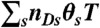, respectively. (iv) Having determined N_D, the random donor lifetime τ can be generated exactly (procedure a) or more efficiently to an excellent approximation for large photon counts (procedure b). In procedure a, a state s is chosen with the probability 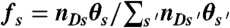and δt is chosen from , which is repeated N_D times and then 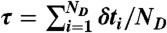. Procedure b is based on approximating the distribution by the gamma-distribution with the exact mean 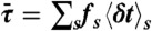and variance 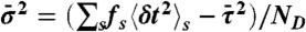; i.e., a single τ is chosen from 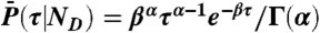, , and . The FRET efficiency is obtained from the photon counts using E = N_A/(N_A + γN_D), where γ is a correction factor used to construct experimental histograms (see SI Text, Fixed energy transfer rate). The random E and τ are then histogrammed.

Recoloring for Diffusing Molecules.

To recolor bursts of photons obtained in free diffusion measurements, we erase photon colors but keep the photon arrival times. For a burst of N photons (irrespective of color) and duration T, new random photon counts N_A, N_D, and lifetime τ are obtained thus: (i) Generate a state trajectory of duration T as above and superimpose it on the experimental burst of photons. (ii) Count the number of photons N_s in each state s that was visited during time T. must equal N. (iii) For each state s, generate the number of donor photons, N_Ds, from the binomial distribution , where ε_s = n_As/(n_As + n_Ds) is the apparent FRET efficiency of state s. (iv) For each state, generate N_Ds delay times δt_is from and calculate their sum 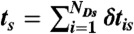. (v) Finally, the random FRET efficiency is E = 1 - N_D/N and the random lifetime in a bin is 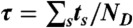, where .

References

- 1.Deniz AA, Mukhopadhyay S, Lemke EA. Single-molecule biophysics: At the interface of biology, physics and chemistry. J R Soc Interface. 2008;5:15–45. doi: 10.1098/rsif.2007.1021. [DOI] [PMC free article] [PubMed] [Google Scholar]
- 2.Schuler B, Eaton WA. Protein folding studied by single-molecule FRET. Curr Opin Struct Biol. 2008;18:16–26. doi: 10.1016/j.sbi.2007.12.003. [DOI] [PMC free article] [PubMed] [Google Scholar]
- 3.Roy R, Hohng S, Ha T. A practical guide to single-molecule FRET. Nat Methods. 2008;5:507–516. doi: 10.1038/nmeth.1208. [DOI] [PMC free article] [PubMed] [Google Scholar]
- 4.Sisamakis E, Valeri A, Kalinin S, Rothwell PJ, Seidel CAM. Accurate single-molecule FRET studies using multiparameter fluorescence detection. Methods Enzymol. 2010;475:455–514. doi: 10.1016/S0076-6879(10)75018-7. [DOI] [PubMed] [Google Scholar]
- 5.Gopich I, Szabo A. Theory of photon statistics in single-molecule Förster resonance energy transfer. J Chem Phys. 2005;122:014707. doi: 10.1063/1.1812746. [DOI] [PubMed] [Google Scholar]
- 6.Gopich IV, Szabo A. Single-molecule FRET with diffusion and conformational dynamics. J Phys Chem B. 2007;111:12925–12932. doi: 10.1021/jp075255e. [DOI] [PubMed] [Google Scholar]
- 7.Gopich IV, Szabo A. Theory of single-molecule FRET efficiency histograms. Adv Chem Phys. 2012;146:245–298. [Google Scholar]
- 8.Eggeling C, et al. Data registration and selective single-molecule analysis using multi-parameter fluorescence detection. J Biotechnol. 2001;86:163–180. doi: 10.1016/s0168-1656(00)00412-0. [DOI] [PubMed] [Google Scholar]
- 9.Yang H, Xie XS. Probing single-molecule dynamics photon by photon. J Chem Phys. 2002;117:10965–10979. [Google Scholar]
- 10.Kalinin S, Valeri A, Antonik M, Felekyan S, Seidel CAM. Detection of structural dynamics by FRET: A photon distribution and fluorescence lifetime analysis of systems with multiple states. J Phys Chem B. 2010;114:7983–7995. doi: 10.1021/jp102156t. [DOI] [PubMed] [Google Scholar]
- 11.Laurence TA, Kong X, Jäger M, Weiss S. Probing structural heterogeneities and fluctuations of nucleic acids and denatured proteins. Proc Natl Acad Sci USA. 2005;102:17348–17353. doi: 10.1073/pnas.0508584102. [DOI] [PMC free article] [PubMed] [Google Scholar]
- 12.Best RB, et al. Effect of flexibility and cis residues in single-molecule FRET studies of polyproline. Proc Natl Acad Sci USA. 2007;104:18964–18969. doi: 10.1073/pnas.0709567104. [DOI] [PMC free article] [PubMed] [Google Scholar]
- 13.Hoffmann A, et al. Mapping protein collapse with single-molecule fluorescence and kinetic synchrotron radiation circular dichroism spectroscopy. Proc Natl Acad Sci USA. 2007;104:105–110. doi: 10.1073/pnas.0604353104. [DOI] [PMC free article] [PubMed] [Google Scholar]
- 14.Sorokina M, Koh HR, Patel SS, Ha T. Fluorescent lifetime trajectories of a single fluorophore reveal reaction intermediates during transcription initiation. J Am Chem Soc. 2009;131:9630–9631. doi: 10.1021/ja902861f. [DOI] [PMC free article] [PubMed] [Google Scholar]
- 15.Haas E, Katchalski-Katzir E, Steinberg IZ. Brownian motion of the ends of oligopeptide chains in solution as estimated by energy transfer between the chain ends. Biopolymers. 1978;17:11–31. [Google Scholar]
- 16.Lakowicz JR. Principles of Fluorescence Spectroscopy. New York: Springer; 2006. p. 446. [Google Scholar]
- 17.Makarov DE, Plaxco KW. Measuring distances within unfolded biopolymers using fluorescence resonance energy transfer: The effect of polymer chain dynamics on the observed fluorescence resonance energy transfer efficiency. J Chem Phys. 2009;131:085105. doi: 10.1063/1.3212602. [DOI] [PMC free article] [PubMed] [Google Scholar]
- 18.Berezhkovskii AM, Szabo A, Weiss GH. Theory of single-molecule fluorescence spectroscopy of two-state systems. J Chem Phys. 1999;110:9145–9150. [Google Scholar]
- 19.Gopich IV, Szabo A. FRET efficiency distributions of multi-state single molecules. J Phys Chem B. 2010;114:15221–15226. doi: 10.1021/jp105359z. [DOI] [PMC free article] [PubMed] [Google Scholar]
- 20.Gillespie DT. Markov Processes: An Introduction for Physical Scientists. San Diego: Academic; 1992. [Google Scholar]
- 21.Gopich IV, Szabo A. Single-macromolecule fluorescence resonance energy transfer and free-energy profiles. J Phys Chem B. 2003;107:5058–5063. [Google Scholar]
- 22.Huan B, Perroud TD, Zare RN. Photon counting histogram: One-photon excitation. Chemphyschem. 2004;5:1523–1531. doi: 10.1002/cphc.200400176. [DOI] [PubMed] [Google Scholar]
- 23.Antonik M, Felekyan S, Gaiduk A, Seidel CAM. Separating structural heterogeneities from stochastic variations in fluorescence resonance energy transfer distributions via photon distribution analysis. J Phys Chem B. 2006;110:6970–6978. doi: 10.1021/jp057257+. [DOI] [PubMed] [Google Scholar]
- 24.Nir E, et al. Shot-noise limited single-molecule FRET histograms: Comparison between theory and experiments. J Phys Chem B. 2006;110:22103–22124. doi: 10.1021/jp063483n. [DOI] [PMC free article] [PubMed] [Google Scholar]
- 25.Gopich IV, Szabo A. Decoding the pattern of photon colors in single-molecule FRET. J Phys Chem B. 2009;113:10965–10973. doi: 10.1021/jp903671p. [DOI] [PMC free article] [PubMed] [Google Scholar]
- 26.Torella JP, Holden SJ, Santoso Y, Hohlbein J, Kapanidis AN. Identifying molecular dynamics in single-molecule fret experiments with burst variance analysis. Biophys J. 2011;100:1568–1577. doi: 10.1016/j.bpj.2011.01.066. [DOI] [PMC free article] [PubMed] [Google Scholar]
- 27.Gopich IV, Szabo A. In: Theory and Evaluation of Single-Molecule Signals. Barkai E, Brown FLH, Orrit M, Yang H, editors. Singapore: World Scientific; 2008. pp. 181–244. [Google Scholar]
- 28.Chung HS, et al. Extracting rate coefficients from single-molecule photon trajectories and FRET efficiency histograms for a fast-folding protein. J Phys Chem A. 2011;115:3642–3656. doi: 10.1021/jp1009669. [DOI] [PMC free article] [PubMed] [Google Scholar]
Associated Data
This section collects any data citations, data availability statements, or supplementary materials included in this article.