Abstract
It is of great interest in modern drug design to accurately calculate the free energies of protein-ligand or nucleic acid-ligand binding. MM-PBSA (Molecular Mechanics-Poisson Boltzmann Surface Area) and MM-GBSA (Molecular Mechanics-Generalized Born Surface Area) have gained popularity in this field. For both methods, the conformational entropy, which is usually calculated through normal mode analysis (NMA), is needed to calculate the absolute binding free energies. Unfortunately, NMA is computationally demanding and becomes a bottleneck of the MM-PB/GBSA-NMA methods. In this work, we have developed a fast approach to estimate the conformational entropy based upon solvent accessible surface area calculations. In our approach, the conformational entropy of a molecule, S, can be obtained by summing up the contributions of all atoms, no matter they are buried or exposed. Each atom has two types of surface areas, solvent accessible surface area (SAS) and buried SAS (BSAS). The two types of surface areas are weighted to estimate the contribution of an atom to S. Atoms having the same atom type share the same weight and a general parameter k is applied to balance the contributions of the two types of surface areas.
This entropy model was parameterized using a large set of small molecules for which their conformational entropies were calculated at the B3LYP/6-31G* level taking the solvent effect into account. The weighted solvent accessible surface area (WSAS) model was extensively evaluated in three tests. For the convenience, TS, the product of temperature T and conformational entropy S, were calculated in those tests. T was always set to 298.15 K through the text. First of all, good correlations were achieved between WSAS TS and NMA TS for 44 protein or nucleic acid systems sampled with molecular dynamics simulations (10 snapshots were collected for post-entropy calculations): the mean correlation coefficient squares (R2) was 0.56. As to the 20 complexes, the TS changes upon binding, TΔS, were also calculated and the mean R2 was 0.67 between NMA and WSAS. In the second test, TS were calculated for 12 proteins decoy sets (each set has 31 conformations) generated by the Rosetta software package. Again, good correlations were achieved for all decoy sets: the mean, maximum, minimum of R2 were 0.73, 0.89 and 0.55, respectively. Finally, binding free energies were calculated for 6 protein systems (the numbers of inhibitors range from 4 to 18) using four scoring functions. Compared to the measured binding free energies, the mean R2 of the six protein systems were 0.51, 0.47, 0.40 and 0.43 for MM-GBSA-WSAS, MM-GBSA-NMA, MM-PBSA-WSAS and MM-PBSA-NMA, respectively. The mean RMS errors of prediction were 1.19, 1.24, 1.41, 1.29 kcal/mol for the four scoring functions, correspondingly. Therefore, the two scoring functions employing WSAS achieved a comparable prediction performance to that of the scoring functions using NMA. It should be emphasized that no minimization was performed prior to the WSAS calculation in the last test.
Although WSAS is not as rigorous as physical models such as quasi-harmonic analysis and thermodynamic integration (TI), it is computationally very efficient as only surface area calculation is involved and no structural minimization is required. Moreover, WSAS has achieved a comparable performance to normal mode analysis. We expect that this model could find its applications in the fields like high throughput screening (HTS), molecular docking and rational protein design. In those fields, efficiency is crucial since there are a large number of compounds, docking poses or protein models to be evaluated. A list of acronyms and abbreviations used in this work is provided for quick reference.
Keywords: Conformational Entropy, Configurational Entropy, WSAS, Solvent Accessible Surface Area, MM-PBSA, MM-GBSA, Binding Free Energy Calculations, Protein Design, Drug Design
1.0 Introduction
1.1 MM-PBSA and MM-GBSA Methods
Free energy prediction is one of the central interests in computational chemistry. With the continually increased computer power, the calculations of free energy changes of biological events, such as protein folding, protein-ligand binding, protein-protein association, have become popular. The methods of calculating free energies and entropies through molecular simulations have been summarized in many reviews.1–7 Among a variety of approaches, MM-PBSA and MM-GBSA have gained popularity owing to their computational efficiency in comparison to the theoretically more rigorous methods such as free energy perturbation and thermodynamic integration.1, 8–16 Critical assessment of the two techniques on modeling protein-ligand binding begins to emerge.17–22
In a typical MM-PB/GBSA calculation, the molecular system of interest is first immersed in a water box and up to tens of nanoseconds molecular dynamics simulations are performed using either the “single trajectory” or the “individual trajectories” protocol.3 In most scenarios, the “single trajectory protocol” is superior to the “individual trajectories protocol” as the former can achieve a better error cancellation. However, when the binding leads to a dramatic conformational change, the ensembles of the receptor, ligand and complex need to be sampled separately (the “individual trajectories” protocol) since the conformational energies and entropies of the receptor and the ligand are significantly different in bound and unbound states.
In the second stage, post free energy analysis is carried out after peeling off the solvent and counter ions. In MM-PB/GBSA theory, the free energy of a molecule is calculated with Eqs. 1–3.
| (1) |
| (2) |
| (3) |
The first term in Eq. 1, Hgas, is replaced with Egas, the gas phase MM energy, as the PV term is negligible for a molecule in condensed phase. <> indicates those energy terms are ensemble averages. The second term in Eq.1, Gsolv consists of two components, the polar and nonpolar solvation free energies (Eq. 2). The polar solvation energy is evaluated either by a PB or a GB model; while the nonpolar solvation free energy is typically estimated with the solvent accessible surface area assuming that the non-polar contribution is proportional to SAS. The nonpolar term accounts for the entropy penalty associated with the reorganization of solvent molecules around the solute and the van der Waals interaction between the solute and solvent. The third term in Eq. (1), the conformational entropy, is further decomposed into three parts, the translational, the rotational and the vibrational entropies (Eq. 3). The translational entropy (Strans) and the rotational entropy (Srot) can be approximated using the standard equations for rigid body translation and rotation,23 and the vibrational part of conformational entropy (Svib) is typically estimated by normal mode analysis assuming that the vibrational movement around the energy well is harmonic. The Svib term can also be obtained by conducting a quasi-harmonic analysis using the MD trajectories in the sampling phase. As we propose to predict the conformational entropic term through solvent accessible surface area calculation, in practice, as long as the two SAS calculations using the same radii, should be combined to avoid double work.
Although successful stories of using MM-PB/GBSA for various biological systems have been reported, both accuracy and efficiency needs to improve for this promising free energy method. As there are many energy terms involved, simply improving one specific term, such as polar and nonpolar components of solvation energy or conformational entropy, may not necessarily improve the overall accuracy of this method. Thus, a step-by-step procedure must be applied to systematically improve the accuracies of all the terms.3 A good molecular mechanical force field for studying both biological and organic molecules with a high quality solvation model is mainly responsible for the success of this method. Certainly it is a challenging and time-consuming procedure to develop a good molecular mechanical force field and an implicit solvation model.
To improve the efficiency of the MM-PB/GBSA method, actions may be taken in both the sampling and the post free energy analysis phases. First of all, one may run MD simulations using an implicit water model, such as GBSA and PBSA, instead of an explicit water model. Although for large molecules, solving the Poisson-Boltzmann equation takes long time, the bottleneck of post free energy phase is to calculate the conformational entropy by NMA.
1.2 Normal Mode Analysis
To conduct normal mode analysis, a molecule must be fully minimized in order to make the harmonic assumption valid. Otherwise, the calculation result is meaningless or has a large computational error. To guarantee a real local minimum or the global minimum is found, a second derivative-based approach, such as Newton Raphson, is usually applied to minimize the RMS gradient to a very low value, otherwise, substantial errors can occur.24, 25 After that, the mass-weighted Hessian matrix is diagonalized and the thermochemical properties are calculated in the same way as frequently done in quantum mechanics. Both the geometrical optimization and normal mode analysis are time-consuming and computer memory demanding for large biological molecules. For example, the CPU time for running conjugate gradient minimization followed by a Newton Raphson minimization (the convergence criterion is the root-mean-square of gradient less than 1.0×10⁻¹² kcal/(molÅ)) are 66, 549 and 1689 minutes for 1BE9 (120 residues), 8GCH (238 residues) and 1A9U (352 residues), respectively. The CPU times for Hessian matrix diagonalization are 99, 701 and 3037 seconds for the three proteins, correspondingly. The above benchmark is based on Intel Xeon X5660 (2.80GHz) CPU. Apparently, full minimization for a middle-sized or large-sized protein is very expensive.
In order to break this bottleneck, a simplified computational strategy was proposed and routinely used in MM-PB/GBSA calculations: only residues within a short distance to the bound ligand, say 8 Å are kept and the other less important residues are truncated. The remaining residues, which are referred to as the active residues, are fully minimized using a distance-dependent dielectric constant.13, 14, 19, 26 A big problem with this truncating strategy is that full minimization may lead to significant conformational changes in the molecular geometry. Kongsted and Ryde recently proposed to add a buffer region surrounding the active residues to maintain the overall molecular geometry and to reduce the standard deviation of the conformational entropy.26 Nevertheless, as we will show later, the truncating strategy tends to underestimate the entropy changes of binding in our tests and should be used with caution.
1.3 Conformation Entropy Calculation
The major goal of this paper is to develop an efficient conformational entropy model for free energy calculations. In the following part of the introduction, we will first elaborate the definitions of conformational entropy and outline the conformational entropy calculations using various methods.
For a molecule in aqueous solution, the total entropy comes from three major contributions, namely, the external entropy due to the translational and rotational degrees of freedom, the internal entropy rooted in vibrational movement, and the entropy due to solvation. The solvation entropy along with the van der Waals interaction between the solute and solvent is well predicted using the solvent accessible surface area as discussed above.27 The vibrational part of conformational entropy is usually evaluated through normal mode analysis and the translational and rotational parts are estimated using rigid body/rotor approximation. Conformational entropy is also called configurational entropy in many publications,2, 28–31 here, we choose to use conformational entropy rather than configurational entropy in order to be consistent with our earlier publications.3, 14, 16 In this work, conformational entropy and configurational entropy are used interchangeably. It should be noted that in some papers conformational entropy is a measure of the number of occupied energy wells and has a different meaning from the conformational entropy defined here.31
Conformational entropy is an important term in the MM-PB/GBSA scoring function. In most cases of the protein-protein, protein-ligand binding, binding affinity is a combined function of binding enthalpy and binding entropy, and high affinity is achieved when both terms contribute favorably to the binding. However, when the binding is dominated by entropic effect, conformational entropy becomes an indispensable term. A scoring function without an entropic term has a biased tendency to select large molecules in virtual screenings.32–34
In molecular docking for which computation efficiency is crucial, conformational entropy is either omitted or simply estimated by the number of frozen rotatable bonds upon ligand binding.35–37 This simple entropy model has been further improved in some docking scoring functions so that the entropy loss of a given rotor depends on its environment.38, 39 However, the chemical nature of rotors which can also affect the entropy is not differentiated. Evidently, entropy models based on the number of frozen rotatable bonds are very crude and they have no discrimination power at all when the major contribution of conformation entropy results from the narrower energy well in the bound state.2 Gilson et al. found that for a set of small host-guest systems, there was no clear correlation between entropy change and the number of rotatable bonds, but the snugness of the guest’s fit in the host’s binding site correlated with entropy loss.40, 41 In another study, Kongsted and Ryde found that the numbers of frozen rotatable bonds have no correlation to the conformational entropies calculated by normal mode analysis for biotin/avidin binding system.26 In another efficient method, Abagyan et al. applied solvent accessible surface area to account for the conformational entropy of the side chains of proteins in conformational searches of peptides and proteins.42 However, their simple model may not be suitable to study protein-ligand binding.
More rigorous methods for calculating configurational entropy include quasi-harmonic analysis (QHA),43, M2 (second generation mining minima) of Gilson et al.44–46, FEP and TI through temperature-derivative calculations.47, non-parametric methods using histogram48 and k-nearest neighbor (kNN),28, 49, hypothetical scanning approach,50, 51 the adaptive anisotropic kernels and minimum information methods by Grubmuller et al.52, 53, and so on.
All the above-mentioned methods except the first two are time consuming and not suitable to be implemented in docking scoring functions or to be used in high throughput screenings. Wlodek et al. recently proposed to use the Hessian matrix generated by the quasi-Newton optimizers rather than the exact analytical Hessian matrix calculated for the optimized compounds to calculate the vibrational entropy.54 However, their method still requires massive structural minimization and therefore is also not suitable to be used in docking studies. To bridge the gap between the efficient but not accurate and the accurate but not efficient approaches, in this work, we proposed a very fast yet reasonably accurate approach for calculating conformational entropy based on solvent accessible surface area calculations. This new model can be used to estimate the conformational entropies of protein models and re-rank docking poses. It can also be integrated into a docking scoring function.
2. Methodology
2.1 Basic Theory
It is known that entropy is an additive property under some approximation, and as such, it is possible to calculate the conformational entropy of a molecule S by adding up the contributions of individual atoms. The interior atoms of a molecule are not fully free to move, therefore, they have less contribution to S than the exposed atoms. However, it is not proper to apply only solvent accessible surface area to measure an atom’s contribution to S since a fully buried atom has zero SAS but it can still make non-negligible contributions to S. For small molecules, this problem may not be severe as most atoms are exposable. However, for macromolecules, omitting the contribution of buried atoms could lead to a significant underestimation of the conformational entropy S since a larger portion of atoms of macromolecules are not accessible to solvent. To address the above problem, we propose to use the following equations to calculate conformational entropy:
| (4) |
| (5) |
Where wi is the weight for atom i; SASi is the solvent accessible surface area of atom i; N is the number of atoms in a molecule; BSASi, the buried solvent accessible surface area of atom i, is calculated using Eq. 5, note that BSAS of atom i is complementary to SAS of atom i; ri is the radius of atom i. The probe radius, rprob, was set to 0.8 Å. We did not use the standard radius of the water probe (1.4 Å), with an aim to explore more hidden areas not accessible by a large water probe. Using rprob of 0.8 Å, a set of encouraging SAS-based models have been developed by us for a variety of molecular properties which include solvation free energy and aqueous solubility.55, 56 The radius parameters used for SAS calculations are adopted from the MSMS program57 and listed in Table 1.
Table 1.
List of the atom type definitions, radius parameters for SAS calculations and the weights of the WSAS entropy model when k in Eq. 4 is set to 0.461.
| Atom Type | Radius (Å) | Weight (cal/(molKÅ2)) | Definition |
|---|---|---|---|
| h1 | 1.2 | 0.1676 | Hydrogen on aliphatic carbon with one electron-withdrawal group |
| h2 | 1.2 | 0.1539 | Hydrogen on aliphatic carbon with two electron-withdrawal groups |
| h3 | 1.2 | 0.1656 | Hydrogen on aliphatic carbon with three electron-withdrawal groups |
| h4 | 1.2 | 0.1708 | Hydrogen on aromatic carbon with one electron-withdrawal group |
| h5 | 1.2 | 0.1551 | Hydrogen on aromatic carbon with two electron-withdrawal groups |
| ha | 1.2 | 0.1525 | Hydrogen bonded to sp1 and sp2 carbon |
| hc | 1.2 | 0.1670 | Hydrogen bonded to sp3 carbon |
| hn | 1.2 | 0.1605 | Hydrogen bonded to nitrogen |
| ho | 1.2 | 0.0984 | Hydrogen bonded to oxygen |
| hs | 1.2 | 0.1225 | Hydrogen bonded to sulfur |
| hp | 1.2 | 0.1274 | Hydrogen bonded to phosphorus |
| hw | same as | ho | Hydrogen of water |
| hx | same as | h3 | Hydrogen on aliphatic carbon next to a positively charged group |
| c | 1.74 | 0.0881 | sp2 carbon in C=O and C=S |
| c1 | 1.74 | 0.0974 | sp1 carbon |
| c2 | 1.74 | 0.0374 | sp2 carbon, aliphatic |
| c3 | 1.74 | −0.0419 | sp3 carbon, aliphatic |
| ca | 1.74 | 0.0352 | sp2 carbon, aromatic |
| cc/cd | 1.74 | 0.0308 | Inner sp2 carbon in conjugated ring systems |
| ce/cf | 1.74 | 0.0321 | Inner sp2 carbon in conjugated chain systems |
| cg/ch | 1.74 | 0.1080 | Inner sp1 carbon in conjugated ring systems |
| cp/cq | 1.74 | 0.0260 | bridge sp2 carbon in biphenyl |
| cu | same as | c2 | sp2 carbon in three-membered rings |
| cv | same as | c2 | sp2 carbon in four-membered rings |
| cx | same as | c3 | sp3 carbon in three-membered rings |
| cy | same as | c3 | sp3 carbon in four-membered rings |
| cz | same as | c2 | sp2 carbon in guanidine |
| n | 1.54 | 0.0194 | sp2 nitrogen in amides |
| n1 | 1.54 | 0.1824 | sp1 nitrogen |
| n2 | 1.54 | 0.1647 | sp2 nitrogen with two substituents, real double bond formed |
| n3 | 1.54 | 0.0393 | sp3 nitrogen with three substituents |
| n4 | 1.54 | −0.0421 | sp3 nitrogen with four substituents |
| na | 1.54 | 0.0585 | sp2 nitrogen with three substituents |
| nb | 1.54 | 0.1271 | sp2 nitrogen in aromatic systems, such as pyridine |
| nc/nd | 1.54 | 0.1426 | Inner sp2 nitrogen in conjugated ring systems |
| ne/nf | 1.54 | 0.1398 | Inner sp2 nitrogen in conjugated chain systems |
| nh | 1.54 | 0.0317 | Amine nitrogen bonded to aromatic rings |
| no | 1.54 | 0.1343 | Nitrogen in nitro groups |
| o | 1.4 | 0.2022 | sp2 oxygen in C=O and COO− |
| oh | 1.4 | 0.2105 | sp3 oxygen in hydroxyl groups |
| os | 1.4 | 0.1804 | sp3 oxygen in ethers and esters |
| s | 2.0 | 0.1592 | sp1 or sp2 sulfur (P=S, C=S, etc.) |
| s4 | 2.0 | 0.1590 | Hypervalent sulfur, three substituents |
| s6 | 2.0 | 0.0900 | Hypervalent sulfur, four substituents |
| sh | 2.0 | 0.1674 | sp3 sulfur in thiol groups |
| ss | 2.0 | 0.1717 | sp3 sulfur other than ‘sh’, two substituents |
| sx | same as | s4 | Conjugated sulfur, three substituents |
| sy | same as | s6 | Conjugated sulfur, four substituents |
| p2 | 2.0 | 0.1821 | sp2 phosphorus (C=P, etc.) |
| p3 | 2.0 | 0.1435 | sp2 phosphorus, three substituents |
| p5 | 2.0 | 0.0846 | hypervalent phosphorus, four substituents |
| pc/pd | same as | p2 | Inner sp2 phosphorus in conjugated ring systems |
| pe/pf | same as | p2 | Inner sp2 phosphorus in conjugated chain systems |
| p4 | same as | p5 | hypervalent phosphorus, three substituents |
| px | same as | p5 | Conjugated phosphorus, three substituents |
| py | same as | p5 | Conjugated phosphorus, four substituents |
| f | 1.6 | 0.1992 | Any fluorine |
| cl | 1.79 | 0.2101 | Any chlorine |
| br | 2.04 | 0.2025 | Any bromine |
| i | 2.15 | 0.2012 | Any iodine |
| si | 2.1 | 0.0594 | Any silicon |
| fe | 2.0 | 0.0000 | Iron |
| consta | 34.7177 | Intercept of multiple linear regression | |
| nt |
k in Eq. 4 is an adjustable parameter to balance the contribution of buried atoms to S. Hereafter, we call conformational entropies calculated by Eqs 4–5 WSAS entropies. To compare the entropy contributions at the energy level, the product of temperature and entropy, TS, is reported throughout the article (T is set to 298.15 K).
To develop a coherent WSAS model for both small molecules and macromolecules, the following strategy is proposed: (1) all the atoms having the same atom type share the same weight; (2) the weigh parameters are derived by linear regression analysis solely using the ab initio entropies of small molecules for a given k parameter; (3) the k parameter is systematically searched from 0 (buried SAS has no contribution to S) to 1 (buried SAS contributes equally to S as SAS) and an ideal value of k is recognized when both the performance of linear regression analysis is satisfactory and the RMS error between the WSAS and NMA TS of macromolecules is as small as possible.
2.2 Data Sets
The objective of this paper is to develop an entropy model for both small organic and large biological molecules. Four types of data sets have been prepared to do parameterization and testing. Data Set I collects 2756 small molecules that come from different sources: molecules used for force field parameterization; those with experimental entropies; model compounds of different organic substituent groups and ring systems listed in CRC Handbook of Chemistry and Physics,58 etc. Data Set I was used to derive the weight parameters in Eq. 4. Since it covers most of if not all the chemical functional groups, our entropy model is unlikely to suffer from the missing parameter problem for arbitrary molecules.
Data Set II has eight protein-ligand systems (PDB Codes: 1A9U, 1ABE, 1AHA, 1FKG, 1FKI, 1HPV, 3PTB and 4PHV), three protein-peptide systems (1BE9, 1HEF and 8GCH), three unbound proteins (1F10, 1KOE and 1LMI), one DNA-ligand complex (195D) and one RNA (422D). For both 1A9U and 1HPV, four truncated systems were generated for each protein by only keeping residues within certain distances (8, 10, 12 and 15 Å) from any atom of the inhibitor. All the structures in this data set were downloaded from the Protein Data Bank (www.rcsb.org).59 MD simulations were performed for each protein or nucleic acid system using the “single trajectory protocol” and 10 snapshots were collected for the post entropy calculations. In total, there are 20×10 bound and 24×10 unbound protein or nucleic acid models prepared (Table 2).
Table 2.
Comparison between NMA and WSAS in TS (T = 298.15 K) calculations for 22 proteins and 2 nucleic acids.
| PDB_ID | Data Type | TS by NMA * | TS by WSAS * | Linear Regression ** | ||
|---|---|---|---|---|---|---|
| R2 | AUE | RMSE | ||||
| Protein-Ligand Complexes | ||||||
| 1A9U | Complex | 3949.05±10.88 | 3990.36±4.29 | 0.83 | 6.41 | 7.24 |
| Ligand | 47.97±0.00 | 46.80±0.02 | 0.00 | 0.01 | 0.02 | |
| Protein | 3922.79±11.72 | 3963.93±4.57 | 0.76 | 7.43 | 8.10 | |
| Binding | 21.71±4.00 | 20.37±1.83 | 0.61 | 2.05 | 2.76 | |
| 1A9U truncated R = 8 Å | Complex | 337.24±2.07 | 281.04±0.92 | 0.61 | 1.20 | 1.40 |
| Ligand | 47.97±0.00 | 46.80±0.01 | 0.00 | 0.01 | 0.01 | |
| Protein | 304.44±2.86 | 248.29±1.39 | 0.54 | 1.94 | 1.98 | |
| Binding | 15.16±3.72 | 14.05±1.40 | 0.55 | 2.52 | 2.79 | |
| 1A9U truncated R = 10 Å | Complex | 497.22±2.16 | 435.34±1.69 | 0.80 | 0.81 | 0.97 |
| Ligand | 47.97±0.00 | 46.80±0.01 | 0.00 | 0.01 | 0.01 | |
| Protein | 465.78±3.03 | 406.17±1.97 | 0.82 | 1.11 | 1.39 | |
| Binding | 16.53±3.07 | 17.63±2.56 | 0.72 | 1.35 | 1.65 | |
| 1A9U truncated R = 12 Å | Complex | 698.80±1.96 | 639.32±1.11 | 0.32 | 1.26 | 1.62 |
| Ligand | 47.97±0.00 | 46.80±0.01 | 0.00 | 0.01 | 0.01 | |
| Protein | 672.33±2.87 | 612.42±1.71 | 0.38 | 1.80 | 2.25 | |
| Binding | 21.49±3.02 | 19.90±2.12 | 0.76 | 1.14 | 1.52 | |
| 1A9U truncated R = 15 Å | Complex | 1125.27±6.65 | 1042.01±2.47 | 0.70 | 3.72 | 4.65 |
| Ligand | 47.97±0.00 | 46.80±0.01 | 0.00 | 0.01 | 0.01 | |
| Protein | 1098.35±3.04 | 1016.40±1.98 | 0.45 | 1.77 | 2.25 | |
| Binding | 21.05±6.89 | 21.19±2.85 | 0.80 | 3.39 | 4.51 | |
| 1ABE | Complex | 3249.00±4.45 | 3278.36±3.18 | 0.63 | 2.04 | 2.74 |
| Ligand | 29.24±0.04 | 28.33±0.02 | 0.78 | 0.02 | 0.03 | |
| Protein | 3232.34±5.41 | 3265.31±2.56 | 0.53 | 2.94 | 3.98 | |
| Binding | 12.59±2.53 | 15.29±1.70 | 0.50 | 1.34 | 1.84 | |
| 1AHA | Complex | 2715.46±5.04 | 2726.63±3.12 | 0.42 | 3.32 | 3.82 |
| Ligand | 25.22±0.00 | 23.51±0.01 | 0.00 | 0.01 | 0.01 | |
| Protein | 2704.94±4.31 | 2715.87±3.26 | 0.37 | 2.99 | 3.48 | |
| Binding | 14.71±3.44 | 12.75±2.17 | 0.80 | 1.44 | 1.65 | |
| 1FKG | Complex | 1232.21±3.38 | 1233.20±1.46 | 0.00 | 3.01 | 3.60 |
| Ligand | 61.60±0.00 | 60.93±0.01 | 0.00 | 0.01 | 0.01 | |
| Protein | 1193.46±3.66 | 1193.86±1.46 | 0.05 | 2.56 | 3.62 | |
| Binding | 22.85±2.45 | 21.59±1.37 | 0.40 | 1.48 | 1.90 | |
| 1FKI | Complex | 2427.95±4.40 | 2440.44±1.87 | 0.07 | 3.63 | 4.28 |
| Ligand | 59.59±0.16 | 62.97±0.13 | 0.99 | 0.03 | 0.04 | |
| Protein | 2384.62±5.92 | 2395.56±1.71 | 0.62 | 4.03 | 4.70 | |
| Binding | 16.26±3.59 | 18.09±2.16 | 0.71 | 1.79 | 2.22 | |
| 1HPV | Complex | 2218.89±5.06 | 2218.38±2.84 | 0.42 | 2.90 | 3.88 |
| Ligand | 67.71±0.02 | 64.29±0.03 | 0.40 | 0.04 | 0.05 | |
| Protein | 2181.30±6.46 | 2182.79±2.71 | 0.37 | 3.93 | 5.27 | |
| Binding | 30.11±4.83 | 28.71±1.03 | 0.67 | 3.38 | 4.00 | |
| 1HPV truncated R = 8 Å | Complex | 406.48±2.66 | 340.28±0.98 | 0.53 | 1.59 | 1.97 |
| Ligand | 67.71±0.02 | 64.29±0.03 | 0.40 | 0.04 | 0.05 | |
| Protein | 359.91±2.91 | 294.81±2.02 | 0.59 | 1.58 | 1.87 | |
| Binding | 21.14±3.46 | 18.82±2.00 | 0.16 | 2.95 | 3.30 | |
| 1HPV truncated R =10 Å | Complex | 582.00±2.88 | 523.89±0.95 | 0.01 | 2.56 | 2.98 |
| Ligand | 67.71±0.02 | 64.29±0.03 | 0.40 | 0.04 | 0.05 | |
| Protein | 540.15±3.14 | 482.95±2.62 | 0.69 | 1.18 | 1.78 | |
| Binding | 25.86±4.99 | 23.35±2.43 | 0.62 | 2.66 | 3.30 | |
| 1HPV truncated R = 12 Å | Complex | 770.23±1.62 | 712.70±0.84 | 0.34 | 1.09 | 1.32 |
| Ligand | 67.71±0.02 | 64.29±0.03 | 0.40 | 0.04 | 0.05 | |
| Protein | 727.74±3.44 | 670.24±1.86 | 0.88 | 1.47 | 1.70 | |
| Binding | 25.22±3.73 | 21.83±1.96 | 0.71 | 1.74 | 2.18 | |
| 1HPV truncated R = 15 ) | Complex | 1135.37±3.60 | 1081.09±1.57 | 0.68 | 1.89 | 2.43 |
| Ligand | 67.71±0.02 | 64.29±0.03 | 0.40 | 0.04 | 0.05 | |
| Protein | 1093.99±6.84 | 1041.29±2.58 | 0.73 | 3.97 | 4.75 | |
| Binding | 26.33±5.54 | 24.49±2.36 | 0.59 | 3.53 | 3.94 | |
| 3PTB | Complex | 2296.37±6.80 | 2302.52±3.27 | 0.74 | 3.60 | 4.32 |
| Ligand | 25.81±0.00 | 24.73±0.01 | 0.00 | 0.08 | 0.00 | |
| Protein | 2286.18±7.17 | 2294.37±3.35 | 0.78 | 3.37 | 4.51 | |
| Binding | 15.63±3.35 | 16.58±0.93 | 0.87 | 2.05 | 2.55 | |
| 4PHV | Complex | 2246.00±5.68 | 2237.64±2.13 | 0.77 | 3.27 | 3.95 |
| Ligand | 78.26±0.38 | 73.52±0.09 | 0.80 | 0.28 | 0.30 | |
| Protein | 2195.60±7.73 | 2192.79±3.34 | 0.85 | 3.98 | 4.83 | |
| Binding | 27.85±8.64 | 28.67±2.76 | 0.86 | 5.65 | 6.21 | |
| Protein-Peptide Complexes | ||||||
| 1BE9 | Complex | 1306.77±4.98 | 1315.13±2.34 | 0.25 | 3.72 | 4.31 |
| Peptide | 84.32±0.29 | 79.40±0.12 | 0.71 | 0.16 | 0.20 | |
| Protein | 1255.68±4.74 | 1259.23±1.35 | 0.07 | 3.60 | 4.58 | |
| Binding | 33.23±6.03 | 23.51±2.33 | 0.82 | 2.81 | 3.33 | |
| 1HEF | Complex | 1179.50±5.45 | 1178.84±2.67 | 0.59 | 3.25 | 3.79 |
| Peptide | 90.76±0.57 | 86.93±0.18 | 0.07 | 0.46 | 0.55 | |
| Protein | 1115.50±4.54 | 1114.67±2.58 | 0.89 | 1.97 | 2.27 | |
| Binding | 26.76±6.74 | 22.76±2.89 | 0.83 | 3.05 | 3.87 | |
| 8GCH | Complex | 2491.53±4.47 | 2489.09±3.05 | 0.33 | 2.99 | 3.68 |
| Peptide | 50.23±0.90 | 46.70±0.30 | 0.82 | 0.50 | 0.62 | |
| Protein | 2467.12±3.30 | 2463.14±3.32 | 0.69 | 1.54 | 1.93 | |
| Binding | 25.82±5.62 | 20.75±2.93 | 0.85 | 1.89 | 2.67 | |
| Protein Receptors | ||||||
| 1FL0 | Protein | 1817.62±6.65 | 1823.04±2.52 | 0.47 | 4.19 | 5.25 |
| 1KOE | Protein | 1859.37±7.42 | 1859.16±2.78 | 0.85 | 4.16 | 4.97 |
| 1LMI | Protein | 1380.58±3.97 | 1381.46±2.38 | 0.89 | 1.63 | 1.89 |
| Nucleic Acids | ||||||
| 195D | Complex | 645.24±2.28 | 658.07±1.45 | 0.80 | 0.98 | 1.19 |
| Ligand | 65.72±0.50 | 57.99±0.08 | 0.63 | 0.38 | 0.43 | |
| DNA | 611.69±3.06 | 625.47±1.81 | 0.42 | 2.17 | 2.34 | |
| Binding | 32.18±3.64 | 25.39±2.10 | 0.50 | 2.01 | 2.57 | |
| 422D | RNA | 668.23±5.02 | 658.56±2.55 | 0.88 | 2.32 | 2.75 |
For each TS by NMA or WSAS, the mean and the RMS deviation were estimated using 10 data points calculated using 10 MD snapshots.
The performance of a linear regression is measured by correlation coefficient square, the average unsigned error (AUE) and root-mean-square error (RMSE).
Data Set III collects 12 protein decoys generated by the Rosetta software package (www.rosettacommons.org). Every protein decoy contains 31 protein models including the crystal one. This data set was used by Lee et al. to evaluate if the state-of-the-art explicit solvent molecular dynamics and implicit solvent free energy calculation can identify the native states from conformational decoys.11 It can be downloaded from http://depts.washington.edu/bakerpg/decoys/. In total, there are 372 protein models in this data set.
Data Set IV is used to evaluate how well the WSAS model in combination with MM-PBSA and MM-GBSA performs in binding free energy calculations. It comprises six protein systems and each has several to tens of inhibitors (the total number of inhibitors is 53). This data set was originally applied by Hou et al. to assess the performance of MM-PBSA and MM-GBSA methods in binding free energy calculations.19
2.3 Ab initio Calculations
Two types of ab initio calculations were performed in this work. For all the molecules in Data Set I, the conformational entropies were calculated using the Jaguar software package of Schrodinger LLC (www.schrodingr.com). Structural optimization was first performed at the B3LYP/6-31G* level taking the aqueous solvent effect into account using a Poisson-Boltzmann model. It has been shown by Baron et al. that solvent has effect on the solute conformational entropy.60 The Hessian matrixes calculated in the first step were used to conduct frequency analysis. The B3LYP/6-31G* frequencies were scaled down using a scaling factor of 0.9945 to better reproduce the experimental values.61 The thermochemical properties at 295.15 K were then calculated using the scaled frequencies. The total entropy S including the contributions from the translational (Strans), rotational (Srot) and vibrational (Svib) movements was taken as the conformational entropy of a molecule.
For the second type of ab initio calculations, the inhibitors of 195D, 1A9U, 1ABE, 1AHA, 1FKG, 1FKI, 1HPV, 3PTB and 4PHV were extracted from the complexes and optimized at the HF/6-31G* level using the Gaussian 03 software package.62 The Merz-Singh-Kollman scheme was used to generate electrostatic potential (ESP).63 Then the RESP (Restrained Electrostatic Potential) charges64 were derived using the RESP program in AMBER 1165 taking the ab initio ESP as input.
2.4 Molecular Dynamics Simulations
The Parm99SB biomolecular force field66, 67 and the General AMBER Force Field (GAFF)68 were used for all the molecular mechanics calculations. The topologies of non-standard residues were prepared using the Antechamber module69 in AMBER 11.65 All MD simulations were performed with the periodic boundary condition to produce isothermal-isobaric ensembles at 300 K using the Sander program in AMBER11. The Particle Mesh Ewald (PME) method70–72 was used to calculate the full electrostatic energy of a unit cell in a macroscopic lattice of repeating images. The integration of the equations of motion was conducted at a time step of 2 femtoseconds. The covalent bonds involving hydrogen atoms were frozen with the SHAKE algorithm.73 Temperature was regulated using the Langevin dynamics74 with the collision frequency of 5 ps−1.75–77 Pressure regulation was achieved with isotropic position scaling and the pressure relaxation time was set to 1.0 picosecond. After the systems were well equilibrated, one nanosecod MD simulations were conducted and 10 snapshots were evenly recorded for the following entropy calculations using NMA and WSAS.
2.5 Normal Model Analysis
The normal mode analysis was conducted using the NAB module of the AMBER11 software package.65 Unless stated otherwise, the whole structures of biomolecules were used for normal mode analysis. For each snapshot, a maximum of 20,000 step-conjugate gradient minimization was first performed and the converge criterion of the gradient was set to 0.0001 kcal/(molÅ). Then a Newton Raphson minimization was performed until either the maximum of 200 steps was reached or the root-mean-square of gradient was less than 1.0×10⁻¹² kcal/(molÅ) The Generalized Born model of Hawkins, Cramer and Truhlar78 was utilized during the minimization and the followed normal mode analysis. The interior and exterior dielectric constants for the GB calculation were set to 1 and 78.5, respectively.
2.6 MM-PBSA/MM-GBSA Binding Free Energy Calculations
The computational details of MM-PBSA and MM-GBSA binding free calculations for Data Set IV were presented in Hou’s work.19 All the energy terms were adopted from the paper except for the conformational entropies, which were recalculated by our WSAS model as described below.
2.7 Model Construction
A two-step systematic search was applied to locate the ideal k parameter in Eq. 4. First of all, k was scanned from 0 to 1.0 at a step of 0.01. In the next fine tuning step, a much smaller step, 0.001, was used to scan a focused range of k. For a given k, the weight parameters were derived by linear regression analysis solely using the ab initio entropies of small molecules. Then the TS of macromolecules in Data Sets II and III were calculated by the current WSAS entropy model. An ideal k was recognized if it led to a good regression performance and simultaneously minimized the difference between the WSAS and NMA TS of macromolecules in Data Sets II and III.
3. Results and Discussion
In this section, we present the linear regression model of conformational entropy based upon solvent accessible surface area calculation, followed by assessing the performance of this model in three tests.
3.1 Development of a Conformational Entropy Model Based on Weighted Solvent Accessible Surface Area
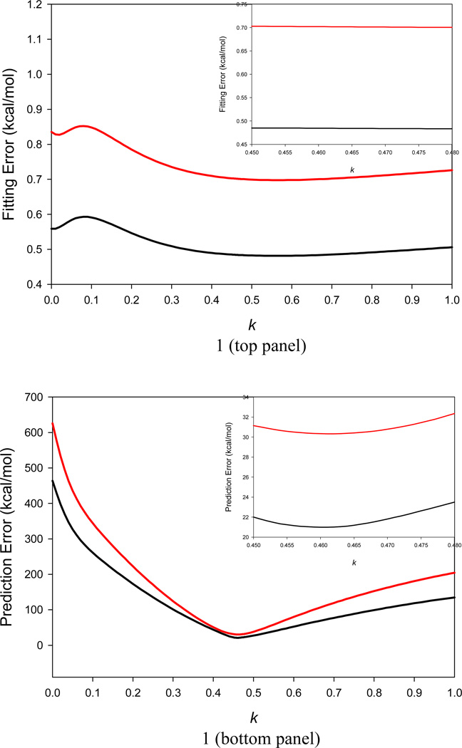
In our algorithm, k in Eq. 4 is a tunable parameter. Without this parameter, it is nearly impossible to develop one single entropy model to make satisfactory predictions for both small molecules and macromolecules. An ideal k value minimizes the RMS error between the WSAS and NMA TS of macromolecules in Data Sets II and III without sacrificing the performance of linear regression for the small molecules in Data Set I. A systemic search was applied to identify the ideal k value. As shown in Figure 1, for small molecules in Data Set I, the AUE and RMSE of TS predicted by the linear regression models do not change dramatically and the maximum difference of RMSE is only 0.01 kcal/mol for k ranged from 0.4 to 0.8 (the minimum of 0.698 kcal/mol is at k = 0.55). While for macromolecules, the RMSE of TS dramatically reduces from 625.8 to 30.3 kcal/mol when k increases from 0 to 0.461; and then the RMSE significantly increases to 204.6 kcal/mol when k approaches 1.0. We finally set k to 0.461 as the ideal value. When k is set to the ideal value, the RMSE of TS for the small molecules in Data Set I is 0.70 kcal/mol, while the RMSE of TS for the macromolecules in Data Sets II and III are 30.3 kcal/mol.
Figure 1.
Application of a two-step systematic search to scan the k parameter in Eq. 4. An ideal k value is recognized when the RMS error of conformational entropy by linear regression analysis for small molecules in Data Set I and the RMS error between the NMA TS and WSAS TS of biomolecules in Data Sets II and III are simultaneously minimized. It is shown that the AUE (black) and RMSE (red) of TS by linear regression analysis using Data Set I are almost unchanged for k from 0.45 to 0.48 (top panel); similarly, the AUE (black) and RMSE (red) between the NMA TS and WSAS TS of biomolecules in Data Sets II and III approach their minimum for k from 0.45 to 0.48 (bottom panel). Thus, the ideal k parameter is set to 0.461.
As illustrated in Figure 1, the buried solvent accessible surface areas make a big contribution to the TS of a given molecule. When this contribution is totally ignored (k = 0), not only the RMSE of TS between WSAS and NMA for macromolecules dramatically increases (625.8 kcal/mol), but also the RMSE of TS between WSAS and ab initio for small molecules (0.84 kcal/mol).
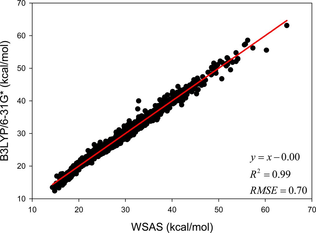
The weight parameters for k = 0.461 are listed in Table 1. The atom type definitions are the same as those for GAFF.68 The performance of the linear regression using Data Set I is demonstrated in Figure 2. The correlation coefficient square is 0.99, and the AUE and RMSE of TS are 0.48 and 0.70 kcal/mol (T = 298.15 K), respectively. The ab initio and WSAS entropies, the SAS and BSAS as well as the SMILES and SLN (Sybyl Line Notation) notations of the 2756 molecules are listed in Table S1 of supporting materials.
Figure 2.
Performance of the WSAS entropy model in reproducing the B3LYP/6-31G* TS for the 2756 small molecules in Data Set I.
It is interesting to investigate the performance of the regression model with all the atom types sharing the same weight. We have found that this simplified SAS model is far inferior to the above WSAS model: the R2 is 0.92 and the AUE and RMSE of TS are 1.24 and 1.73 kcal/mol, respectively. Therefore the approach to allowing different atom types have different weights is well justified.
The contribution of translational and rotational entropies dominates the conformational entropies of a small molecule as indicated by Table S1. However, it is not justified to neglect the contribution of vibrational entropy: the correlation coefficient square is only 0.79 between the translational/rotational entropies and the total entropies for Data Set I. As long as a macromolecule is concerned, the dominated component of conformational entropy is from vibrational frequencies and the vibrational entropy is certainly not negligible.
Is it a better idea to model vibrational entropy separately? To find out the answer, we constructed a WSAS model only using the vibrational entropies (Table S1). It is clear that the regression model is also inferior to the best WSAS model which calibrates the translational, rotational and vibrational entropies altogether: R2 = 0.97 and the AUE and RMSE of TS are 0.67 and 0.96 kcal/mol, respectively. In another word, the AUE and RMSE increase about 40% compared to the best WSAS model (k = 0.461).
Compared to normal mode analysis, the CPU time of WSAS is negligible. For the three aforementioned protein systems, the average CPU times are 0.7, 1.8 and 5.1 seconds for 1BE9, 8GCH and 1A9U, respectively.
3.2 Model Validation for Small Molecules
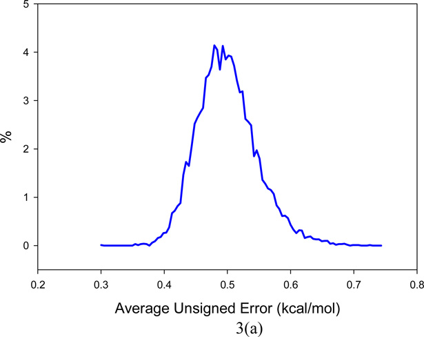
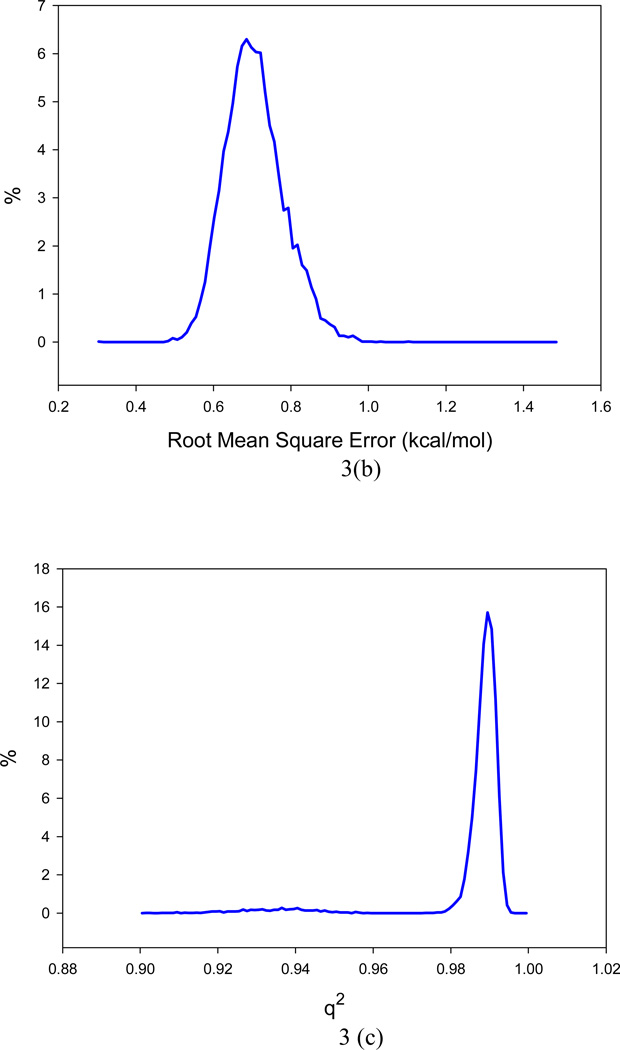
In order to test the predictability of the WSAS model described above, two validation analyses were conducted for Data Set I. First of all, the leave-one-out (LOO) analysis achieves a correlation coefficient square (q2), AUE and RMSE of 0.99, 0.50 and 0.79 kcal/mol, respectively. Then a 10,000 cross validation (CV) runs were performed. For each run, 5% entries were randomly selected to enter the test set and their entropies were calculated with the model generated using the remaining entries. The mean q2, AUE and RMSE for the 10,000 cross validation are 0.99 ± 0.01, 0.50 ± 0.05 and 0.76 ± 0.23 respectively. The distributions of cross validation q2, AUE and RMSE are shown in Figure 3. As the AUE and RMSE in both validation tests are only marginally larger than those of full regression analysis and the q2 of LOO and CV are essentially equal to the correlation coefficient square of the full regression analysis (R2), we are confident that our WSAS model is very reliable.
Figure 3.
Distributions of the key statistical parameters of the 10,000 cross-validation runs on the best WSAS model (k=0.461): (a) Average Unsigned Error of TS, (b) Root-mean-square Error of TS, (c) q2.
3.3 Model Validation for Macromolecules
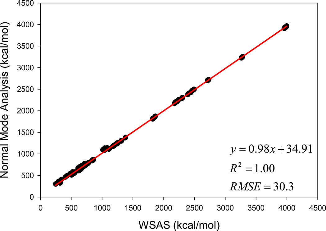
It should be emphasized that the weight parameters in Eq. 4 were determined using the small molecule data set (Data Set I). The macromolecule data sets (Data Sets II and III) were only used to determine the ideal value of the k parameter. The performance of the WSAS model in reproducing the NMA TS of macromolecules is illustrated in Figure 4. The correlation coefficient square is 1.00, and the AUE and RMSE are 21.0 and 30.3 kcal/mol, respectively.
Figure 4.
How the WSAS entropies reproduce the TS by normal mode analysis for 812 protein and nucleic acid models in Data Sets II and III.
For the normal mode analysis, attention must be paid to the first several frequencies. The first six frequencies are for the translational and rotational modes. Their values should be close to 0.0. If one or several negative vibrational frequencies are observed, it suggests that the structure is optimized to a transition state, or to a higher order point. To guarantee a local minimum or the global minimum is found, two types of algorithms, conjugate gradient followed by Newton Raphson were used to minimize the RMS gradient to a very low value. In this work, the final RMS gradients are all smaller than 1.0×10⁻¹² kcal/(molÅ). In our experience, when RMS gradients are larger than 1.0×10⁻⁴ kcal/(molÅ), the calculated thermodynamics properties may not be reliable.
3.4 Application of the WSAS Entropy in Protein Structure Prediction
In the following section, the WSAS model was challenged in more realistic applications. In the first test, we examine how WSAS performs in reproducing the NMA entropies of different conformations sampled by MD simulations for a single macromolecule. For each protein or nucleic acid of Data Set II, 10 snapshots were collected in one nanosecond MD simulations. The statistics of the means and the root-mean-square deviations of TS are summarized in Table 2. Although the absolute difference of conformational entropies by WSAS and NMA can be large, reasonably good correlations are achieved in most cases. The mean correlation coefficient squares R2 is 0.56 for 44 macromolecules (24 receptors and 20 complexes), while R2 of 20 ligands is 0.34 between WSAS and NMA. However, R2 for the ligands can be dramatically increased to 0.69 if those rigid ligands with the RMS deviations of TS by normal mode analysis smaller than 0.03 kcal/mol are eliminated. The R2, AUE and RMSE of the linear regressions analysis are listed in Table 2.
The changes of TS in ligand binding were calculated using the following equation: TΔS = T(Scomplex − Sreceptor − Sligand). Good correlations were achieved between the WSAS TΔS and NMA TΔS as shown in Table 2. The mean R2, AUE and RMSE of 20 protein and nucleic systems are 0.67, 2.41 and 2.94 kcal/mol, respectively. The significantly better correlation of TΔS than that of the TS of macromolecules is understandable since the former has achieved a better error cancellation.
The root-mean-square deviations (RMSD) of the NMA and WSAS TS were calculated and listed in Table 2. For the macromolecules (receptors and complexes), the average, minimum and maximum RMSD of NMA are 4.3, 0.3 and 11.7, respectively; while the three deviations are 2.1, 0.1 and 4.6 kcal/mol correspondingly for WSAS. As long as the RMSD for the binding entropy TΔS are compared, the deviations for WSAS (mean = 2.1, min = 0.9, max = 2.9 kcal/mol) are also much smaller than those for NMA (mean = 4.5, min = 2.4, max = 8.6 kcal/mol). It is also encouraging that the RMSE of linear regression analysis are always smaller than the RMS deviations of TS by NMA for biomolecules.
For large macromolecules, the widely used normal mode analysis is very time-consuming. A common strategy in MM-PB/GBSA analysis is to truncate the residues that are relatively far away from the binding site in order to save computer time. Here we investigated how this strategy affects the calculation results using two protein systems, MAP kinase P38 (PDB code: 1A9U)79 and HIV-1 protease (PDB code: 1HPV).80 Each protein was truncated by only keeping residues within 8, 10, 12 and 15 Å of any atoms of the inhibitors. As demonstrated by Table 2, the TS by NMA can be dramatically different between untruncated and truncated proteins. For the first truncating scheme (truncating radius R = 8 Å), the TΔS of ligand binding by NMA are underestimated by 6.6 and 8.9 kcal/mol for 1A9U and 1HPV, respectively. For the second truncating scheme (truncating radius R = 10 Å), the TΔS are underestimated by 5.2 and 4.2 kcal/mol for 1A9U and 1HPV, respectively. Even when the truncating radius is as large as 15 Å, the binding entropy is still underestimated by more than 3.8 kcal/mol for 1HPV. Therefore, the strategy of truncating less important residues to enhance computational efficiency should be exercised with great caution.
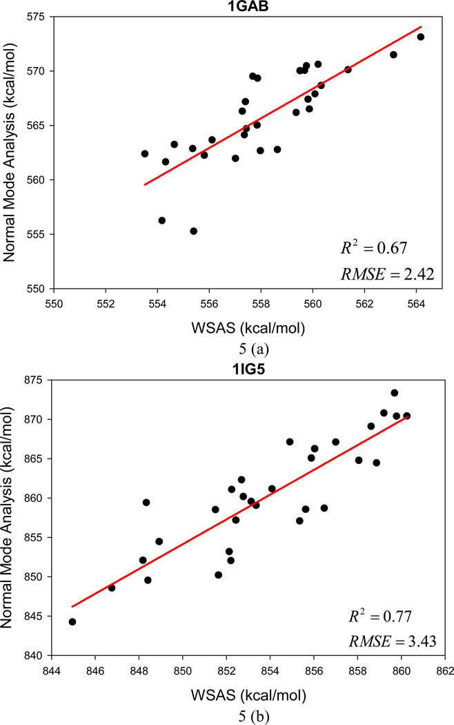
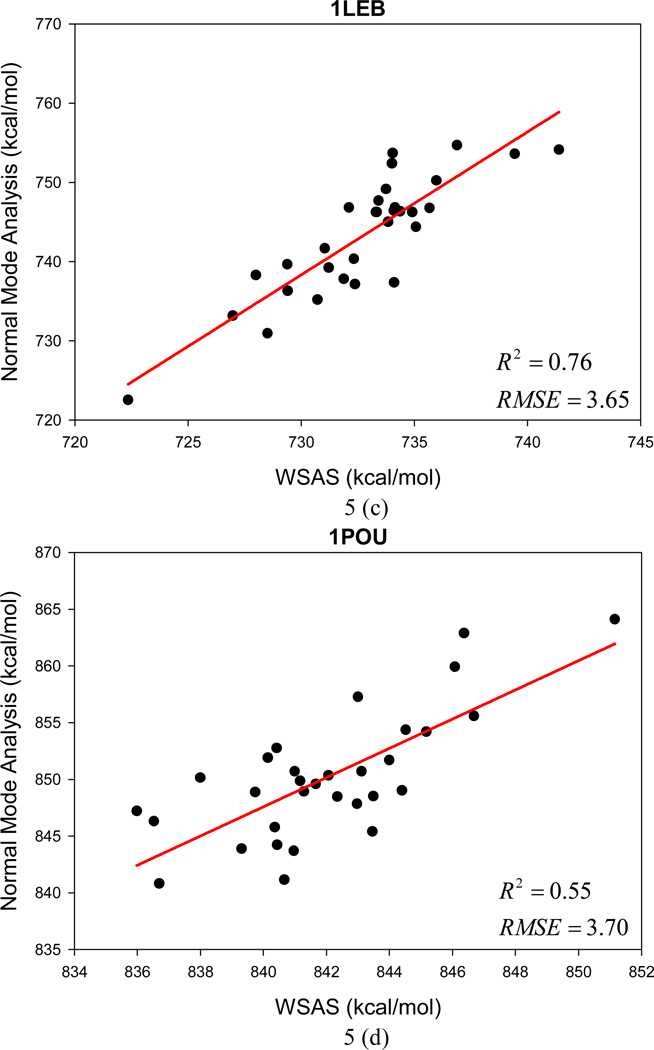
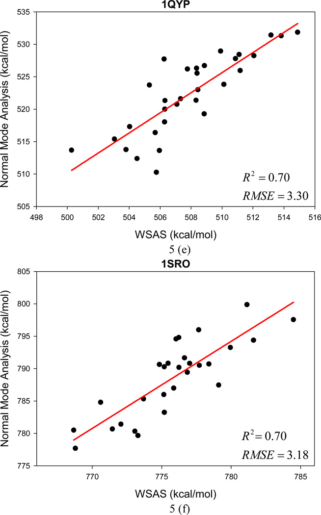
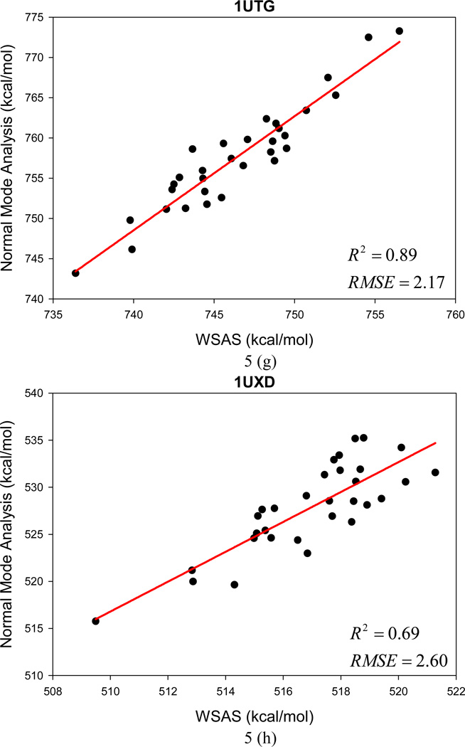
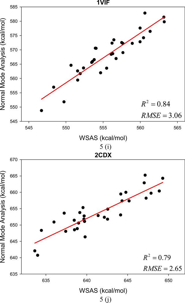
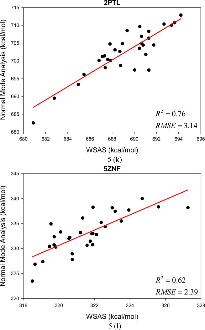
Unlike Data Set II for which the entries were sampled by MD simulations, Data Set III collects conformational decoys generated by the program of conducting ab initio protein predictions in the Rosetta software package (www.rosettacommons.org). An encouraging performance has been achieved by WSAS in comparison to NMA calculated by the NAB program. The mean R2 for 12 small protein systems is 0.73, and the AUE and RMSE of TS are 2.4 and 3.0 kcal/mol, respectively. Figure 5 illustrates the performance of linear regressions between WSAS and NMA for each protein decoy set.
Figure 5.
The performance of the WSAS entropy model in reproducing the TS by normal mode analysis for 12 protein decoys in Data Set III
In summary, our WSAS entropy model has achieved a very good performance in predicting the conformational entropies for a variety of protein and nucleic acids systems. Given the fact that WSAS is computationally very efficient, it could be implemented in protein structural prediction or protein design packages to take the entropic effect into account.
3.5 Application of the WSAS Model in Rational Drug Design
Unlike the above sections of using entropies by normal mode analysis as references, in this evaluation test, we investigate how WSAS in combination with MM-PB/GBSA performs when compared to experimental binding free energies. In a recent work by Hou et al,19 different MM-PBSA and MM-GBSA schemes, such as using different GB models and utilizing different intrinsic dielectric constants in solvation free energies calculations, were explored for six protein-ligand systems. Each protein-ligand system has several to tens of inhibitors and their binding free energies are known. Four binding free energy calculation schemes, namely, MM-PBSA-NMA, MM-PBSA-WSAS, MM-GBSA-NMA and MM-GBSA-WSAS, were assessed with the experimental data. All the energetic terms except the conformational entropies by WSAS are adopted from the work of Hou et al.19 It should be pointed out that the WSAS entropies were calculated using the MD sampled conformations without further minimization.
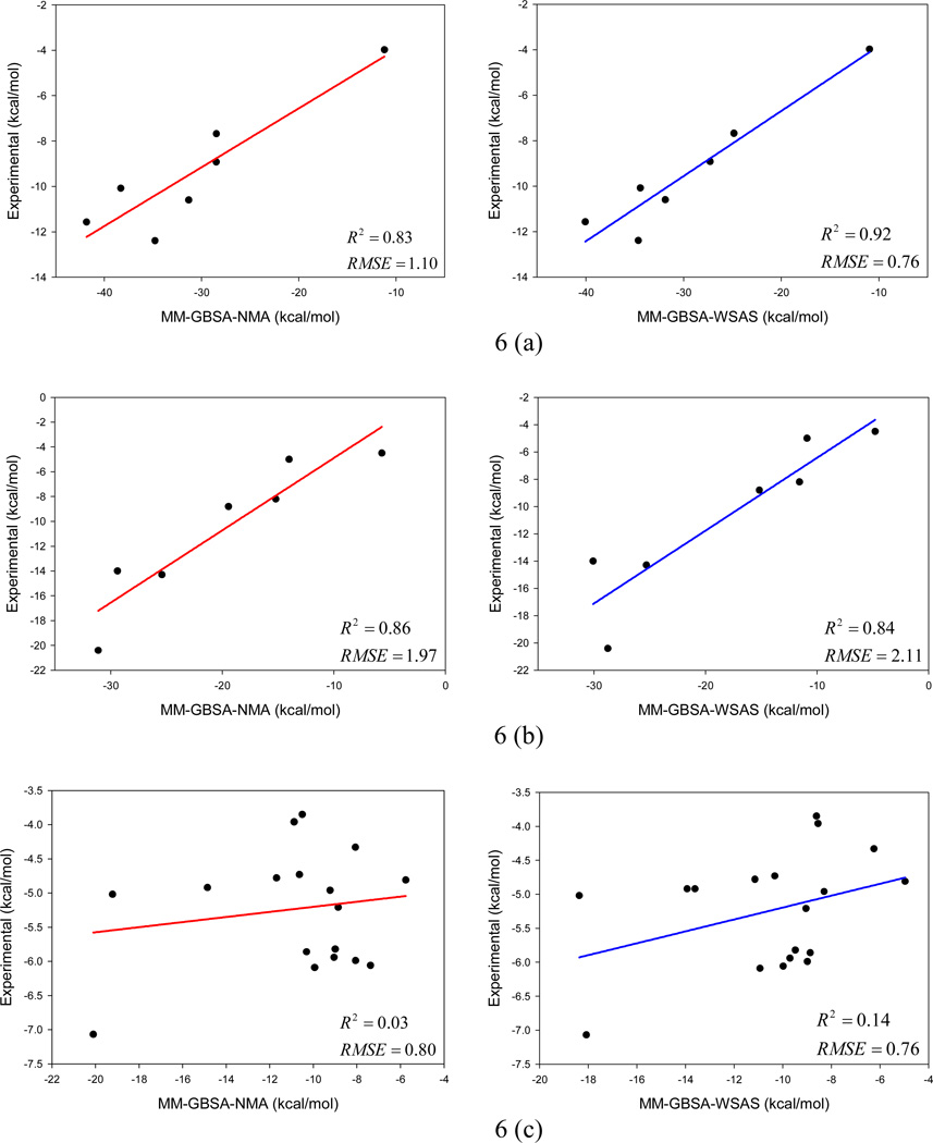
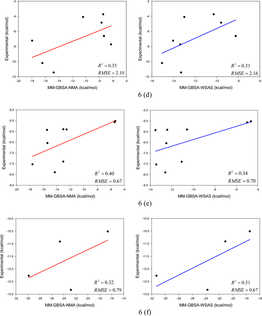
The multiple linear regression analysis results for the two MM-GBSA and two MM-PBSA schemes are listed in Tables 3 and 4, respectively. The linear fitting performance of the two MM-GBSA schemes is shown in Figure 6, and that of the two MM-PBSA schemes is illustrated in Figure S1 of the supporting materials. As shown in Figures 6 and S1, the absolute binding free energies of the first two systems (α-thrombin and avidin) are poorly predicted; however, very good correlations are achieved between the MM-PB/GBSA and experimental binding free energies for these two systems. The seven biotin/avidin complexes were also extensively studied by Genheden et al. using eight solvation models (two PBSA, four GBSA and two MM/3D-RISM solvation models).81 Their finding is similar to ours: the variation of solvation free energies of the eight models is very extensive and the differences are up to 49.7 kcal/mol; therefore, the absolute binding free energies of this particular protein system are difficult to predict, while the relative binding free energies can be well predicted (R2 range from 0.59 to 0.93). In drug design, it is more meaningful to correctly rank the binding affinities of a set of ligands than to predict their absolute binding free energies. The poor correlation between the predicted and experimental binding free energies of cytochrome C is understandable: the range of the experimental binding free energies is very narrow and 80% data points fall between −6.2 and −4.2 kcal/mol. The RMSE of prediction for this system are actually very good as shown in Tables 3 and 4.
Table 3.
Performance of two MM-GBSA protocols in binding free energy calculations*.
| Protein Systems | #Ligand | MM-GBSA-NMA | MM-GBSA-WSAS | ||||
|---|---|---|---|---|---|---|---|
| AUE | RMSE | R2 | AUE | RMSE | R2 | ||
| α-thrombin | 7 | 0.93 | 1.10 | 0.83 | 0.61 | 0.76 | 0.92 |
| avidin | 7 | 1.72 | 1.97 | 0.86 | 1.64 | 2.11 | 0.84 |
| cytochrome C peroxidase | 18 | 0.70 | 0.80 | 0.03 | 0.68 | 0.76 | 0.14 |
| neuraminidase | 8 | 1.95 | 2.10 | 0.35 | 1.78 | 2.16 | 0.31 |
| P450cam | 9 | 0.55 | 0.67 | 0.40 | 0.58 | 0.70 | 0.34 |
| Penicillopepsin** | 4 | 0.64 | 0.79 | 0.32 | 0.58 | 0.67 | 0.51 |
| Mean | 1.08 | 1.24 | 0.47 | 0.98 | 1.19 | 0.51 | |
AUE and RMSE are in kcal/mol.
Three ligands, f5, f6 and f7 in the paper of Hou et al. (Ref. 19) were eliminated because of apparently wrong molecular structures.
Table 4.
Performance of two MM-PBSA protocols in binding free energy calculations*.
| Protein Systems | #Ligand | MM-PBSA-NMA | MM-PBSA-WSAS | ||||
|---|---|---|---|---|---|---|---|
| AUE | RMSE | R2 | AUE | RMSE | R2 | ||
| α-thrombin | 7 | 1.40 | 1.57 | 0.64 | 1.21 | 1.42 | 0.70 |
| avidin | 7 | 1.62 | 1.92 | 0.87 | 2.43 | 2.58 | 0.77 |
| cytochrome C peroxidase | 18 | 0.66 | 0.77 | 0.09 | 0.65 | 0.76 | 0.11 |
| neuraminidase | 8 | 1.75 | 1.92 | 0.46 | 1.87 | 2.09 | 0.36 |
| P450cam | 9 | 0.54 | 0.64 | 0.46 | 0.66 | 0.75 | 0.25 |
| Penicillopepsin** | 4 | 0.89 | 0.94 | 0.03 | 0.66 | 0.86 | 0.18 |
| Mean | 1.14 | 1.29 | 0.42 | 1.25 | 1.41 | 0.40 | |
AUE and RMSE are in kcal/mol.
Three ligands, f5, f6 and f7 in the paper of Hou et al. (Ref. 19) were eliminated because of apparently wrong molecular structures.
Figure 6.
Comparison of two MM-GBSA protocols, MM-GBSA-NMA (left) and MM-GBSA-WSAS (right) in binding free energy calculations for six protein-ligand systems: (a) α-thrombin, (b) avidin, (c) cytochrome C peroxidase, (d) neuraminidase, (e) P450cam, and (f) penicillopepsin.
The means and uncertainties of energy terms other than TΔS by WSAS were listed in the work of Hou et al.19 The uncertainty of WSAS TS measured by the root-mean-square deviation of block averages are summarized as follows: the mean root-mean-square deviations are 0.05, 0.03, 0.02, 0.02, 0.02, and 0.06 kcal/mol for α-thrombin, avidin, cytochrome C peroxidase, neuraminidase, P450cam and penicillopepsin, respectively.
It is encouraging that MM-GBSA-WSAS and MM-PBSA-WSAS achieve a comparable performance to that of two scoring functions employing NMA as demonstrated by Tables 3 and 4. Interestingly, the performance of the two PBSA schemes is inferior to that of the two GBSA schemes, which might suggest the PBSA model Hou et al. used needs further parameterization. As this surprising result is unlikely related to conformational entropy, further discussion on this topic is beyond the scope of this paper.
3.6 Further Development
We have pointed out in the Methodology section that the weight parameters in Eq. 4 were derived solely using the B3LYP/6-31G* entropies of 2756 small molecules in Data Set I, while the k parameter was determined using both Data Set I and two macromolecular data sets (Data Sets II and III). Because of this, our WSAS model is somewhat independent of molecular mechanical force fields. Thus, we anticipate that the k parameter does not deviate from 0.461 too much for a harmonic force field other than AMBER Parm99SB.
We must point out that the WSAS model inherits some limitations of normal mode analysis, for example the anharmonic effect is totally ignored. However, the quality of the weight parameters may not be reduced as the anharmonicity is not significant for small molecules. The ideal k parameter may change when the conformational entropies of biological molecules in Data Sets II and III include the anharmonicity and high-order correlations. We plan to calculate the conformational entropies of biological molecules using the non-parametric kNN approach and to reoptimize the k parameter.
Although WASA has achieved an encouraging performance in several stringent tests, it is still improvable as the q2 of some cross-validation runs are lower than the mean by up to 0.1 (Figure 3C). We plan to add more model compounds into Data Set I and oversample the populations of the building blocks of biomolecules, bioactive compounds as well as approved and experimental drugs. Secondly, atom type definition schemes will be explored by adding and/or modifying some atom types to improve the regression performance. We expect that the redeveloped WSAS model will be much more reliable and suitable to calculate the entropies of biomolecules as well as the entropic changes of protein-ligand and nucleic acid-ligand binding.
4. Conclusions
In this work, we proposed an approach of calculating conformational entropies using both the solvent accessible surface areas (SAS) and the buried SAS. The introduction of the tunable parameter k in Eq. 4, which balances the contribution of the buried SAS to the conformational entropy of a molecule, facilitates us to develop a general SAS-based entropy model for both small molecules and macromolecules. The ideal value of k, 0.461, was determined by a systematic search. This mode is very efficient since only SAS calculation is involved and geometric minimization is not needed prior to the entropy calculation.
The WSAS model has been extensively validated using both the small molecular and macromolecular data sets. The applications of WSAS in protein structural prediction and binding free energy calculations have been discussed. The overall performance of the WSAS model is very encouraging: the mean correlation coefficients between the WSAS and NMA are 0.56 and 0.73 for conformational decoys of biological molecules sampled by MD and Rosetta, respectively; in combination with MM-PBSA and MM-GBSA, the WSAS entropy model achieves a comparable performance to that of NMA in reproducing the experimental binding affinities of six protein-ligand systems. How to further improve the WSAS model has also been discussed. Given the fact that the WSAS is computationally very efficient, we expect the WSAS model to have great applications in both protein structural modeling and structure-based drug design.
Supplementary Material
Acknowledgments
This work was supported by National Institutes of Health grants R21GM097617 (J. Wang, P.I.) and R01GM79383 (Y. Duan, P.I.). We are grateful to TeraGrid for the computational time (TG-CHE090098, J. Wang, P.I.) and the research support from OpenEye Scientific Software, Santa Fe, NM.
Abbreviations
- S
Conformational Entropy
- TS
Product of Temperature T Times Conformation Entropy S
- SAS
Solvent Accessible Surface Area
- BSAS
Buried Solvent Accessible Surface Area
- WSAS
Weighted Solvent Accessible Surface Area
- MM-PBSA
Molecular Mechanics-Poisson Boltzmann Surface Area
- MM-GBSA
Molecular Mechanics-Generalized Born Surface Area
- NMA
Normal Mode Analysis
- QHA
Quasi-harmonic Analysis
- kNN
k-nearest neighbor
- QSAR
Quantitative Structure – Activity Relationship
- MLR
Multiple Linear Regressions
- LOO
Leave-One-Out
- CV
Cross Validation
- R2
Square of Regression Coefficient
- q2
Square of Cross-Validation Regression Coefficient
- AUE
Average Unsigned Error
- RMSE
Root-Mean-Square Error
Footnotes
Supporting Information Available:
The SMILES and SLN notions of 2756 small molecules in Data Set I are listed in Table S1. This table also lists the ab initio TS at the B3LYP/6-31G* level and the predicted TS by the WSAS model. Performance of the two MM-PBSA protocols (MM-PBSA-NMA and MM-PBSA-WSAS) is shown in Figure S1. This material is available free of charge via the Internet at http://pubs.acs.org.
References
- 1.Kollman PA, Massova I, Reyes C, Kuhn B, Huo S, Chong L, Lee M, Lee T, Duan Y, Wang W, Donini O, Cieplak P, Srinivasan J, Case DA, Cheatham TE., III Calculating structures and free energies of complex molecules: Combining molecular mechanics and continuum models. Acc. Chem. Res. 2000;33:889–897. doi: 10.1021/ar000033j. [DOI] [PubMed] [Google Scholar]
- 2.Gilson MK, Given JA, Bush BL, McCammon JA. The statistical-thermodynamic basis for computation of binding affinities: A critical review. Biophys. J. 1997;72:1047–1069. doi: 10.1016/S0006-3495(97)78756-3. [DOI] [PMC free article] [PubMed] [Google Scholar]
- 3.Wang JM, Hou TJ, Xu XJ. Recent Advances in Free Energy Calculations with a Combination of Molecular Mechanics and Continuum Models. Curr. Comput.-Aided Drug Des. 2006;2:287–306. [Google Scholar]
- 4.Jorgensen WL. Free-Energy Calculations - A breakthrough for modeling organic-chemistry in solution. Acc. Chem. Res. 1989;22:184–189. [Google Scholar]
- 5.Beveridge DL, Dicapua FM. Free-energy via molecular simulation - applications to chemical and biomolecular systems. Annu. Rev. Biophys. Biophys. Chem. 1989;18:431–492. doi: 10.1146/annurev.bb.18.060189.002243. [DOI] [PubMed] [Google Scholar]
- 6.Meirovitch H. Recent developments in methodologies for calculating the entropy and free energy of biological systems by computer simulation. Curr. Opin. Struct. Biol. 2007;17:181–186. doi: 10.1016/j.sbi.2007.03.016. [DOI] [PubMed] [Google Scholar]
- 7.Boresch S, Tettinger F, Leitgeb M, Karplus M. Absolute binding free energies: A quantitative approach for their calculation. J. Phys. Chem. B. 2003;107:9535–9551. [Google Scholar]
- 8.Massova I, Kollman PA. Combined molecular mechanical and continuum solvent approach (MM-PBSA/GBSA) to predict ligand binding. Perspect. Drug Discov. Des. 2000;18:113–135. [Google Scholar]
- 9.Swanson JMJ, Henchman RH, McCammon JA. Revisiting free energy calculations: A theoretical connection to MM/PBSA and direct calculation of the association free energy. Biophys. J. 2004;86:67–74. doi: 10.1016/S0006-3495(04)74084-9. [DOI] [PMC free article] [PubMed] [Google Scholar]
- 10.Srinivasan J, Cheatham TE, Cieplak P, Kollman PA, Case DA. Continuum solvent studies of the stability of DNA, RNA, and phosphoramidate - DNA helices. J. Am. Chem. Soc. 1998;120:9401–9409. [Google Scholar]
- 11.Lee MR, Tsai J, Baker D, Kollman PA. Molecular dynamics in the endgame of protein structure prediction. J. Mol. Biol. 2001;313:417–430. doi: 10.1006/jmbi.2001.5032. [DOI] [PubMed] [Google Scholar]
- 12.Huo SH, Wang JM, Cieplak P, Kollman PA, Kuntz ID. Molecular dynamics and free energy analyses of cathepsin D-inhibitor interactions: Insight into structure-based ligand design. J. Med. Chem. 2002;45:1412–1419. doi: 10.1021/jm010338j. [DOI] [PubMed] [Google Scholar]
- 13.Wang W, Lim WA, Jakalian A, Wang J, Wang JM, Luo R, Bayly CT, Kollman PA. An analysis of the interactions between the Sem-5 SH3 domain and its ligands using molecular dynamics, free energy calculations, and sequence analysis. J. Am. Chem. Soc. 2001;123:3986–3994. doi: 10.1021/ja003164o. [DOI] [PubMed] [Google Scholar]
- 14.Wang JM, Morin P, Wang W, Kollman PA. Use of MM-PBSA in reproducing the binding free energies to HIV-1 RT of TIBO derivatives and predicting the binding mode to HIV-1 RT of efavirenz by docking and MM-PBSA. J. Am. Chem. Soc. 2001;123:5221–5230. doi: 10.1021/ja003834q. [DOI] [PubMed] [Google Scholar]
- 15.Wang W, Donini O, Reyes CM, Kollman PA. Biomolecular simulations: Recent developments in force fields, simulations of enzyme catalysis, protein-ligand, protein-protein, and protein-nucleic acid noncovalent interactions. Ann. Rev. Biophys. Biomol. Struct. 2001;30:211–243. doi: 10.1146/annurev.biophys.30.1.211. [DOI] [PubMed] [Google Scholar]
- 16.Wang JM, Kang XS, Kuntz ID, Kollman PA. Hierarchical database screenings for HIV-1 reverse transcriptase using a pharmacophore model, rigid docking, solvation docking, and MM-PB/SA. J. Med. Chem. 2005;48:2432–2444. doi: 10.1021/jm049606e. [DOI] [PubMed] [Google Scholar]
- 17.Kuhn B, Gerber P, Schulz-Gasch T, Stahl M. Validation and use of the MM-PBSA approach for drug discovery. J. Med. Chem. 2005;48:4040–4048. doi: 10.1021/jm049081q. [DOI] [PubMed] [Google Scholar]
- 18.Yang TY, Wu JC, Yan CL, Wang YF, Luo R, Gonzales MB, Dalby KN, Ren PY. Virtual screening using molecular simulations. Proteins. 2011;79:1940–1951. doi: 10.1002/prot.23018. [DOI] [PMC free article] [PubMed] [Google Scholar]
- 19.Hou T, Wang J, Li Y, Wang W. Assessing the performance of the MM/PBSA and MM/GBSA methods. 1. The accuracy of binding free energy calculations based on molecular dynamics simulations. J. Chem. Info. Model. 2011;51:69–82. doi: 10.1021/ci100275a. [DOI] [PMC free article] [PubMed] [Google Scholar]
- 20.Hou T, Wang J, Li Y, Wang W. Assessing the performance of the molecular mechanics/Poisson Boltzmann surface area and molecular mechanics/generalized Born surface area methods. II. The accuracy of ranking poses generated from docking. J. Comput. Chem. 2011;32:866–877. doi: 10.1002/jcc.21666. [DOI] [PMC free article] [PubMed] [Google Scholar]
- 21.Weis A, Katebzadeh K, Soderhjelm P, Nilsson I, Ryde U. Ligand affinities predicted with the MM/PBSA method: Dependence on the simulation method and the force field. J. Med. Chem. 2006;49:6596–6606. doi: 10.1021/jm0608210. [DOI] [PubMed] [Google Scholar]
- 22.Mobley DL, Dill KA. Binding of small-molecule ligands to proteins: "what you see" is not always "what you get". Structure. 2009;17:489–498. doi: 10.1016/j.str.2009.02.010. [DOI] [PMC free article] [PubMed] [Google Scholar]
- 23.McQuarrie DA, Simon JD. Molecular Thermodynamics. Sausalito, CA 94965: University Science Books; 1999. [Google Scholar]
- 24.Bahar I, Rader AJ. Coarse-grained normal mode analysis in structural biology. Curr. Opin. Struct. Biol. 2005;15:586–592. doi: 10.1016/j.sbi.2005.08.007. [DOI] [PMC free article] [PubMed] [Google Scholar]
- 25.Yang L, Song G, Jernigan RL. How well can we understand large-scale protein motions using normal modes of elastic network models? Biophys. J. 2007;93:920–929. doi: 10.1529/biophysj.106.095927. [DOI] [PMC free article] [PubMed] [Google Scholar]
- 26.Kongsted J, Ryde U. An improved method to predict the entropy term with the MM/PBSA approach. J. Comput.-Aided Mol. Des. 2009;23:63–71. doi: 10.1007/s10822-008-9238-z. [DOI] [PubMed] [Google Scholar]
- 27.Genheden S, Mikulskis P, Hu LH, Kongsted J, Soderhjelm P, Ryde U. Accurate predictions of nonpolar solvation free energies require explicit consideration of binding-site hydration. J. Am. Chem. Soc. 2011;133:13081–13092. doi: 10.1021/ja202972m. [DOI] [PubMed] [Google Scholar]
- 28.Hnizdo V, Tan J, Killian BJ, Gilson MK. Efficient calculation of configurational entropy from molecular simulations by combining the mutual-information expansion and nearest-neighbor methods. J. Comput. Chem. 2008;29:1605–1614. doi: 10.1002/jcc.20919. [DOI] [PMC free article] [PubMed] [Google Scholar]
- 29.Jusuf S, Loll PJ, Axelsen PH. Configurational entropy and cooperativity between ligand binding and dimerization in glycopeptide antibiotics. J. Am. Chem. Soc. 2003;125:3988–3994. doi: 10.1021/ja027780r. [DOI] [PubMed] [Google Scholar]
- 30.Harpole KW, Sharp KA. Calculation of configurational entropy with a Boltzmann-Quasiharmonic model: The origin of high-affinity protein-ligand binding. J. Phys. Chem. B. 2011;115:9461–9472. doi: 10.1021/jp111176x. [DOI] [PubMed] [Google Scholar]
- 31.Chang CEA, Chen W, Gilson MK. Ligand configurational entropy and protein binding. Proc. Natl. Acad. Sci. USA. 2007;104:1534–1539. doi: 10.1073/pnas.0610494104. [DOI] [PMC free article] [PubMed] [Google Scholar]
- 32.Liu L, Yang C, Guo QX. A study on the enthalpy-entropy compensation in protein unfolding. Biophys. Chem. 2000;84:239–251. doi: 10.1016/s0301-4622(00)00130-7. [DOI] [PubMed] [Google Scholar]
- 33.Livesay DR, Dallakyan S, Wood GG, Jacobs DJ. A flexible approach for understanding protein stability. Febs Lett. 2004;576:468–476. doi: 10.1016/j.febslet.2004.09.057. [DOI] [PubMed] [Google Scholar]
- 34.Li DW, Khanlarzadeh M, Wang JB, Huo SH, Brcuschweiler R. Evaluation of configurational entropy methods from peptide folding-unfolding simulation. J. Phys. Chem. B. 2007;111:13807–13813. doi: 10.1021/jp075220e. [DOI] [PubMed] [Google Scholar]
- 35.Bohm HJ. The development of a simple empirical scoring function to estimate the binding constant for a protein-ligand complex of known three-dimensional structure. J. Comput.-Aided Mol. Des. 1994;8:243–256. doi: 10.1007/BF00126743. [DOI] [PubMed] [Google Scholar]
- 36.Wang R, Lai L, Wang S. Further development and validation of empirical scoring functions for structure-based binding affinity prediction. J. Comput.-Aided Mol. Des. 2002;16:11–26. doi: 10.1023/a:1016357811882. [DOI] [PubMed] [Google Scholar]
- 37.Rarey M, Kramer B, Lengauer T, Klebe G. A fast flexible docking method using an incremental construction algorithm. J. Mol. Biol. 1996;261:470–489. doi: 10.1006/jmbi.1996.0477. [DOI] [PubMed] [Google Scholar]
- 38.Eldridge MD, Murray CW, Auton TR, Paolini GV, Mee RP. Empirical scoring functions: I. The development of a fast empirical scoring function to estimate the binding affinity of ligands in receptor complexes. J. Comput.-Aided Mol. Des. 1997;11:425–445. doi: 10.1023/a:1007996124545. [DOI] [PubMed] [Google Scholar]
- 39.Giordanetto F, Cotesta S, Catana C, Trosset JY, Vulpetti A, Stouten PF, Kroemer RT. Novel scoring functions comprising QXP, SASA, and protein side-chain entropy terms. J. Chem. Info. Comput. Sci. 2004;44:882–893. doi: 10.1021/ci0499626. [DOI] [PubMed] [Google Scholar]
- 40.Chang CE, Gilson MK. Free energy, entropy, and induced fit in host-guest recognition: calculations with the second-generation mining minima algorithm. J. Am. Chem. Soc. 2004;126:13156–13164. doi: 10.1021/ja047115d. [DOI] [PubMed] [Google Scholar]
- 41.Chen W, Chang CE, Gilson MK. Calculation of cyclodextrin binding affinities: energy, entropy, and implications for drug design. Biophys. J. 2004;87:3035–3049. doi: 10.1529/biophysj.104.049494. [DOI] [PMC free article] [PubMed] [Google Scholar]
- 42.Abagyan R, Totrov M. Biased probability Monte Carlo conformational searches and electrostatic calculations for peptides and proteins. J. Mol. Biol. 1994;235:983–1002. doi: 10.1006/jmbi.1994.1052. [DOI] [PubMed] [Google Scholar]
- 43.Karplus M, Kushick JN. Method for estimating the configurational entropy of macromolecules. Macromolecules. 1981;14:325–332. [Google Scholar]
- 44.Chang CE, Gilson MK. Tork: Conformational analysis method for molecules and complexes. J. Comput. Chem. 2003;24:1987–1998. doi: 10.1002/jcc.10325. [DOI] [PubMed] [Google Scholar]
- 45.Chen W, Chang CE, Gilson MK. Concepts in receptor optimization: targeting the RGD peptide. J. Am. Chem. Soc. 2006;128:4675–4684. doi: 10.1021/ja056600l. [DOI] [PubMed] [Google Scholar]
- 46.Chang CE, Potter MJ, Gilson MK. Calculation of molecular configuration integrals. J. Phys. Chem. B. 2003;107:1048–1055. [Google Scholar]
- 47.Peter C, Oostenbrink C, van Dorp A, van Gunsteren WF. Estimating entropies from molecular dynamics simulations. J. Chem. Phys. 2004;120:2652–2661. doi: 10.1063/1.1636153. [DOI] [PubMed] [Google Scholar]
- 48.Killian BJ, Kravitz JY, Gilson MK. Extraction of configurational entropy from molecular simulations via an expansion approximation. J. Chem. Phys. 2007;127:024107. doi: 10.1063/1.2746329. [DOI] [PMC free article] [PubMed] [Google Scholar]
- 49.Hnizdo V, Darian E, Fedorowicz A, Demchuk E, Li S, Singh H. Nearest-neighbor nonparametric method for estimating the configurational entropy of complex molecules. J. Comput. Chem. 2007;28:655–668. doi: 10.1002/jcc.20589. [DOI] [PubMed] [Google Scholar]
- 50.Cheluvaraja S, Meirovitch H. Calculation of the entropy and free energy of peptides by molecular dynamics simulations using the hypothetical scanning molecular dynamics method. J. Chem. Phys. 2006;125:24905. doi: 10.1063/1.2208608. [DOI] [PubMed] [Google Scholar]
- 51.Meirovitch H. Methods for calculating the absolute entropy and free energy of biological systems based on ideas from polymer physics. J. Mol. Recognit. 2010;23:153–172. doi: 10.1002/jmr.973. [DOI] [PMC free article] [PubMed] [Google Scholar]
- 52.Hensen U, Grubmuller H, Lange OF. Adaptive anisotropic kernels for nonparametric estimation of absolute configurational entropies in high-dimensional configuration spaces. Phys. Rev. E. 2009;80:011913. doi: 10.1103/PhysRevE.80.011913. [DOI] [PubMed] [Google Scholar]
- 53.Hensen U, Lange OF, Grubmuller H. Estimating absolute configurational entropies of macromolecules: the minimally coupled subspace approach. PloS one. 2010;5:e9179. doi: 10.1371/journal.pone.0009179. [DOI] [PMC free article] [PubMed] [Google Scholar]
- 54.Wlodek S, Skillman AG, Nicholls A. Ligand Entropy in Gas-Phase, Upon Solvation and Protein Complexation. Fast Estimation with Quasi-Newton Hessian. J. Chem. Theory Comput. 2010;6:2140–2152. doi: 10.1021/ct100095p. [DOI] [PubMed] [Google Scholar]
- 55.Wang J, Hou T, Xu X. Aqueous solubility prediction based on weighted atom type counts and solvent accessible surface areas. J. Chem. Inf. Model. 2009;49:571–581. doi: 10.1021/ci800406y. [DOI] [PubMed] [Google Scholar]
- 56.Wang JM, Krudy G, Hou TJ, Zhang W, Holland G, Xu XJ. Development of reliable aqueous solubility models and their application in druglike analysis. J. Chem. Inf. Model. 2007;47:1395–1404. doi: 10.1021/ci700096r. [DOI] [PubMed] [Google Scholar]
- 57.Sanner MF, Olson AJ, Spehner JC. Reduced surface: An efficient way to compute molecular surfaces. Biopolymers. 1996;38:305–320. doi: 10.1002/(SICI)1097-0282(199603)38:3%3C305::AID-BIP4%3E3.0.CO;2-Y. [DOI] [PubMed] [Google Scholar]
- 58.Lide DRE. CRC Handbook of Chemistry and Physics. Ed. 86. Boca Raton, FL: CRC Press; 2005. pp. 4–523. [Google Scholar]
- 59.Berman HM, Westbrook J, Feng Z, Gilliland G, Bhat TN, Weissig H, Shindyalov IN, Bourne PE. The Protein Data Bank. Nucleic Acids Res. 2000;28:235–242. doi: 10.1093/nar/28.1.235. [DOI] [PMC free article] [PubMed] [Google Scholar]
- 60.Baron R, Bakowies D, van Gunsteren WF. Principles of carbopeptoid folding: a molecular dynamics simulation study. J. Pept. Sci. 2005;11:74–84. doi: 10.1002/psc.597. [DOI] [PubMed] [Google Scholar]
- 61.Scott AP, Radom L. Harmonic vibrational frequencies: An evaluation of Hartree-Fock, Moller-Plesset, quadratic configuration interaction, density functional theory, and semiempirical scale factors. J. Phys. Chem. 1996;100:16502–16513. [Google Scholar]
- 62.Frisch MJ, Trucks GW, Schlegel HB, Scuseria GE, Robb MA, Cheeseman JR, Montgomery JJA, Vreven T, Kudin KN, Burant JC, Millam JM, Iyengar SS, Tomasi J, Barone V, Mennucci B, Cossi M, Scalmani G, Rega N, Petersson GA, Nakatsuji H, Hada M, Ehara M, Toyota K, Fukuda R, Hasegawa J, Ishida M, Nakajima T, Honda Y, Kitao O, Nakai H, Klene M, Li X, Knox JE, Hratchian HP, Cross JB, Bakken V, Adamo C, Jaramillo J, Gomperts R, Stratmann RE, Yazyev O, Austin AJ, Cammi R, Pomelli C, Ochterski JW, Ayala PY, Morokuma K, Voth GA, Salvador P, Dannenberg JJ, Zakrzewski VG, Dapprich S, Daniels AD, Strain MC, Farkas O, Malick DK, Rabuck AD, Raghavachari K, Foresman JB, Ortiz JV, Cui Q, Baboul AG, Clifford S, Cioslowski J, Stefanov BB, Liu G, Liashenko A, Piskorz P, Komaromi I, Martin RL, Fox DJ, Keith T, Al-Laham MA, Peng CY, Nanayakkara A, Challacombe M, Gill PMW, Johnson B, Chen W, Wong MW, Gonzalez C, Pople JA. Gaussian 03. Wallingford, CT: Gaussian, Inc; 2004. [Google Scholar]
- 63.Singh UC, Kollman PA. An Approach to Computing Electrostatic Charges for Molecules. J. Comput. Chem. 1984;5:129–145. [Google Scholar]
- 64.Bayly CI, Cieplak P, Cornell WD, Kollman PA. A well-behaved electrostatic potential based method using charge restraints for deriving atomic charges-the RESP model. J. Phys. Chem. 1993;97:10269–10280. [Google Scholar]
- 65.Case DA, Darden TA, Cheatham ITE, Simmerling C, Wang J, Duke RE, Luo R, Walker RC, Zhang W, Merz KM, Roberts B, Wang B, Hayik S, Roitberg A, Seabra G, Kolossvary I, Wong KF, Paesani F, Vanicek J, Liu J, Wu X, Brozell SR, Steinbrecher T, Gohlke H, Cai Q, Ye X, Wang J, Hsieh MJ, Cui G, Roe DR, Mathews DH, Seetin MG, Sagui C, Babin V, Luchko T, Gusarov S, Kovalenko A, Kollman PA. AMBER11. San Francisco, CA: University of California; 2010. [Google Scholar]
- 66.Wang J, Cieplak P, Kollman PA. How well does a restrained electrostatic potential (RESP) model perform in calculating conformational energies of organic and biological molecules? J. Comput. Chem. 2000;21:1049–1074. [Google Scholar]
- 67.Hornak V, Abel R, Okur A, Strockbine B, Roitberg A, Simmerling C. Comparison of multiple Amber force fields and development of improved protein backbone parameters. Proteins. 2006;65:712–725. doi: 10.1002/prot.21123. [DOI] [PMC free article] [PubMed] [Google Scholar]
- 68.Wang J, Wolf RM, Caldwell JW, Kollman PA, Case DA. Development and testing of a general amber force field. J. Comput. Chem. 2004;25:1157–1174. doi: 10.1002/jcc.20035. [DOI] [PubMed] [Google Scholar]
- 69.Wang JM, Wang W, Kollman PA, Case DA. Automatic atom type and bond type perception in molecular mechanical calculations. J. Mol. Graph. Modell. 2006;25:247–260. doi: 10.1016/j.jmgm.2005.12.005. [DOI] [PubMed] [Google Scholar]
- 70.Darden T, Perera L, Li L, Pedersen L. New tricks for modelers from the crystallography toolkit: the particle mesh Ewald algorithm and its use in nucleic acid simulations. Structure. 1999;7:R55–R60. doi: 10.1016/s0969-2126(99)80033-1. [DOI] [PubMed] [Google Scholar]
- 71.Essmann U, Perera L, Berkowitz ML, Darden T, Lee H, Pedersen LG. A smooth particle mesh Ewald method. J. Chem. Phys. 1995;103:8577–8593. [Google Scholar]
- 72.Sagui C, Pedersen LG, Darden TA. Towards an accurate representation of electrostatics in classical force fields: Efficient implementation of multipolar interactions in biomolecular simulations. J. Chem. Phys. 2004;120:73–87. doi: 10.1063/1.1630791. [DOI] [PubMed] [Google Scholar]
- 73.Miyamoto S, Kollman PA. Settle - an analytical version of the Shake and Rattle algorithm for rigid water models. J. Comput. Chem. 1992;13:952–962. [Google Scholar]
- 74.Uberuaga BP, Anghel M, Voter AF. Synchronization of trajectories in canonical molecular-dynamics simulations: observation, explanation, and exploitation. J. Chem. Phys. 2004;120:6363–6374. doi: 10.1063/1.1667473. [DOI] [PubMed] [Google Scholar]
- 75.Izaguirre JA, Catarello DP, Wozniak JM, Skeel RD. Langevin stabilization of molecular dynamics. J. Chem. Phys. 2001;114:2090–2098. [Google Scholar]
- 76.Larini L, Mannella R, Leporini D. Langevin stabilization of molecular-dynamics simulations of polymers by means of quasisymplectic algorithms. J. Chem. Phys. 2007;126:104101. doi: 10.1063/1.2464095. [DOI] [PubMed] [Google Scholar]
- 77.Loncharich RJ, Brooks BR, Pastor RW. Langevin dynamics of peptides - the frictional dependence of Isomerization rates of N-acetylalanyl-N'-methylamide. Biopolymers. 1992;32:523–535. doi: 10.1002/bip.360320508. [DOI] [PubMed] [Google Scholar]
- 78.Hawkins GD, Cramer CJ, Truhlar DG. Parametrized models of aqueous free energies of solvation based on pairwise descreening of solute atomic charges from a dielectric medium. J. Phys. Chem. 1996;100:19824–19839. [Google Scholar]
- 79.Wang ZL, Canagarajah BJ, Boehm JC, Kassisa S, Cobb MH, Young PR, Abdel-Meguid S, Adams JL, Goldsmith EJ. Structural basis of inhibitor selectivity in MAP kinases. Struct. Fold. Des. 1998;6:1117–1128. doi: 10.1016/s0969-2126(98)00113-0. [DOI] [PubMed] [Google Scholar]
- 80.Kim EE, Baker CT, Dwyer MD, Murcko MA, Rao BG, Tung RD, Navia MA. Crystal-structure of HIV-1 protease in complex with VX-478, a potent and orally bioavailable inhibitor of the enzyme. J. Am. Chem. Soc. 1995;117:1181–1182. [Google Scholar]
- 81.Genheden S, Luchko T, Gusarov S, Kovalenko A, Ryde U. An MM/3D-RISM Approach for Ligand Binding Affinities. J. Phys. Chem. B. 2010;114:8505–8516. doi: 10.1021/jp101461s. [DOI] [PubMed] [Google Scholar]
Associated Data
This section collects any data citations, data availability statements, or supplementary materials included in this article.


