On the Nondifferential Misclassification of a Binary Confounder

Abstract

Consider a study with binary exposure, outcome, and confounder, where the confounder is nondifferentially misclassified. Epidemiologists have long accepted the unproven but oft-cited result that, if the confounder is binary, then odds ratios, risk ratios, and risk differences that control for the mismeasured confounder will lie between the crude and the true measures. In this paper we provide an analytic proof of the result in the absence of a qualitative interaction between treatment and confounder, and demonstrate via counterexample that the result need not hold when there is such a qualitative interaction. We also present an analytic proof of the result for the effect of treatment among the treated, and describe extensions to measures conditional on or standardized over other covariates.

Observational studies of any design require accurate measurement of and adjustment for confounders in order to estimate causal effects without bias. However, misclassification of confounders is a pervasive—indeed some would say ubiquitous—problem that has been written about extensively.^1–12 While misclassification and measurement error continue to be the subject of much research, the problem of describing and bounding bias due to misclassification is considered solved, at least in some simple settings. In 1980, Greenland¹³ argued that adjustment for a binary nondifferentially mismeasured confounder reduces the bias due to the confounder and therefore produces a partially adjusted effect measure that falls between the crude (i.e. unadjusted) and true (i.e. adjusted by the true confounder) measures. We hereafter refer to this as the “partial-control” result. Savitz and Baron¹⁴ presented a framework for quantifying the percent of the bias of the crude effect measure that remains after partial adjustment for a nondifferentially mismeasured confounder. They found, via simulations, that this “residual confounding” decreases with increasing sensitivity and specificity. Fung and Howe¹⁵ presented evidence from simulations showing that adjustment for a nondifferentially mismeasured polytomous confounder similarly accomplishes partial control for confounding, but Brenner¹⁶ corrected the record by showing that adjustment for a non-differential misclassified polytomous confounder may induce greater bias than failing to adjust for the confounder at all, or it may change the direction of the bias. He argued that appeal should be made to the partial-control result only for a binary confounder. Though this result has never been proven, it has been cited without qualification in methodological and applied work from 1980 onward.^{11,12,17–20}

We prove that the partial-control result holds for binary confounders under the additional assumption that the effect of the confounder on the outcome is in the same direction among the treated and the untreated (i.e., there is no qualitative interaction between the treatment and the confounder). We demonstrate via counterexample that the result does not necessarily hold when this assumption is violated. We also prove that the partial-control result holds for the effect of treatment on the treated, i.e. when estimates are standardized by the distribution of the confounder among the exposed rather than in the entire population. Our remarks and results apply equally to effects on the risk difference, risk ratio, and odds ratio scales. The assumption of no qualitative interaction between treatment and confounder will likely hold in most applications in epidemiology, and therefore adjusting for a nondifferentially misclassified binary confounder will usually reduce the bias of the effect estimate relative to the crude, unadjusted estimate. If there is reason to believe, however, that qualitative interaction may exist between treatment and a mismeasured confounder, then adjusting for the mismeasured confounder may not reduce bias.

BACKGROUND AND NOTATION

We assume that a “true” 2 × 2 × 2 table represents the effect of a binary exposure, A, on a binary outcome, Y, stratified by a binary covariate, C. We assume for now that C suffices to control for all confounding of the effect of A on Y, so that adjustment for C allows identification of the true effect. As discussed below, the results here also hold if adjustment for other covariates is necessary to control for confounding. We assume that C is not observed and that C′, an imperfect measure of C, is observed instead. An “observed” table represents the association between A on Y stratified by C′. Let e = P [C′= 1|C = 1] be the sensitivity and f = P [C′= 0|C = 0] be the specificity. Then P [C′= 1] = e · P [C = 1] + (1 − f)P [C = 0]. We assume that all measurement error is nondifferential, i.e. P [C′= d|C = c, A = a, Y = y] = P [C′= d|C = c] for all a, and y. A diagram depicting the relationships among the variables is given in Figure 1.

Figure 1.

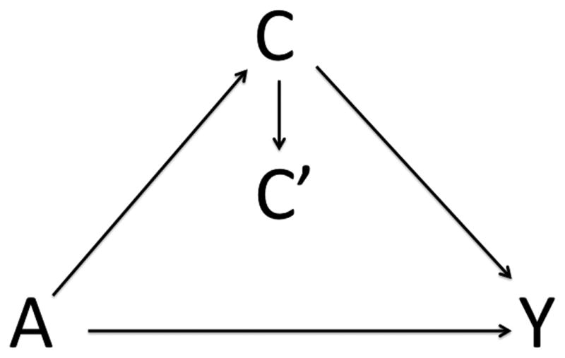
Relations among A, Y, and C

We will call effect measures that adjust for C′“observed adjusted” measures,¹⁶ those that adjust for C “true,” and those that collapse over C “crude.” Let Y₁ be the counterfactual outcome under exposure A = 1, i.e. the outcome we would have observed if, possibly contrary to fact, a subject had received exposure A = 1. Let Y₀ be the counterfactual outcome under exposure A = 0. We make the consistency assumption that Y_a= Y when A = a. The true effect measures are formulated in terms of the distributions of these counterfactuals, e.g. the true risk difference (RD) is RD_true,= E[Y₁] − E[Y₀]. For no subject do we observe both Y₁ and Y₀; we observe only the counterfactual corresponding to the subject’s actual exposure. However, within levels of C, subjects are effectively randomized with respect to treatment (by the assumption that C is the sole confounder), so E[Y₁|A = 0, C = c] = E[Y₁|A = 1, C = c] = E[Y|A = 1, C = c]. Therefore both E[Y₁] and E[Y₀] can be calculated by standardizing by C: E[Y_a] = E[Y|A = a, C = 1]P [C = 1] + E[Y|A = a, C = 0]P [C = 0], for a = 0, 1. We will denote by E_C′[Y|A = a] the corresponding expression standardized by C′ instead of C: E_C′ [Y|A = a] = E[Y|A = a, C′ = 1]P [C′ = 1] + E[Y|A = a, C′ = 0]P [C′ = 0], for a = 0, 1. The observed adjusted measures are formulated in terms of the means standardized by C′; for example the observed adjusted RD is RD_obs = E_C′ [Y|A = 1] − E_C′ [Y|A = 0], and the crude measures are formulated in terms of the unstandardized conditional means: RD_crude = E[Y|A = 1] − E[Y|A = 0].

Our interest is in comparing the observed adjusted risk difference, given above, risk ratio (RR), RR_obs = E_C′ [Y|A = 1]/E_C′ [Y|A = 0], and odds ratio (OR), OR_obs = {E_C′ [Y|A = 1] (1 − E_C′ [Y|A = 0])}/{E_C′ [Y|A = 0] (1 − E_C′ [Y|A = 1])}, to the corresponding true and crude measures.

RESULTS

The partial-control result need not hold in general, but we prove that it always holds under an additional assumption about the joint distribution of Y, A, and C. We define monotonicity of conditional expectations and then present our main result. If E[Y|A = a, C = 0] ≤ E[Y|A = a, C = 1] for both a = 0 and a = 1, then we say that E[Y|A, C] is nondecreasing in C. If E[Y|A = a, C = 0] ≥ E[Y|A = a, C = 1] for both a = 0 and a = 1 then we say that E[Y|A, C] is nonincreasing in C. If E[Y|A, C] is either nonincreasing or nondecreasing in C then it is monotonic in C. In what follows we will refer to this property simply as monotonicity in C, and to monotonicity of E[Y|A, C′] in C′ as monotonicity in C′. Monotonicity in C requires that the confounder affects the outcome in the same direction among the exposed and unexposed. If the confounder has a protective effect among one exposure group and a harmful effect among the other, i.e. if there is a qualitative interaction between A and C, then monotonicity will be violated.

Result 1 For A and C binary and C′ nondifferentially misclassified, if E[Y|A, C] is monotonic in C, then the observed adjusted effect lies between the crude and true effects on the RD, RR, and OR scales.

For the proof see the Appendix.

Not all departures from monotonicity will result in observed adjusted effects that fall outside of the range of the crude and the true effects, but without monotonicity there is no guarantee that the partial-control result will hold. Unfortunately, because the true C is unobserved, it is often impossible to verify the assumption of monotonicity. One must instead rely on subject matter knowledge to determine whether monotonicity is a reasonable assumption.

It is possible to test monotonicity in C′ in the observed data, and monotonicity in C entails monotonicity in C′(see Appendix). Therefore if E[Y|A, C′] is not monotonic in C′, then the assumption on which the partial-control result depends is not satisfied. On the other hand, monotonicity in C′ does not guarantee monotonicity in C.

If E[Y|A, C′] is monotonic in C′, subject-matter understanding of the relationships among Y, A, and C may allow researchers to assume that monotonicity holds or is violated. For monotonicity to hold, C must either increase the risk of Y among both exposed and unexposed subjects, or decrease the risk of Y among both the exposed and unexposed. In order for monotonicity to be violated, C must exhibit a qualitative interaction with A such that it has a protective effect among either the exposed or the unexposed and a harmful effect among the other exposure group. For example, let Y be hypertension, A be type 2 diabetes (a chronic condition positively associated with hypertension), and C be thiazide (a drug commonly prescribed to treat hypertension). While thiazide lowers the risk of hypertension in the general population, it is known to increase blood glucose levels and thereby exacerbate diabetes among diabetics.²¹ It is possible that, though protective in the non-diabetic stratum, thiazide may increase the risk of hypertension in the diabetic group by aggravating their condition. This would constitute a violation of the monotonicity assumption.

Counterexample to the partial-control result when monotonicity is violated

The counterexample given in Table 1 demonstrates that when the assumption of monotonicity is violated, the observed adjusted effect need not lie between the crude and true. In this example, E [Y|A = 1, C = c] is decreasing in c while E [Y|A = 0, C = c] is increasing in c. The observed adjusted effect measure is less than both the crude and the true effect measures (and thus not between the two) on the RD, RR, and OR scales. The ordering of the risk ratios, RR_obs < RR_crude < RR_true, indicates that the observed adjusted risk ratio is more biased than the crude, no matter what measure of bias is used. (This is because the crude measure is between the observed adjusted and the true measures and is therefore closer to the true measure on any scale. This occurred for the RR in this example, but other examples in which monotonicity is violated can be found in which RD and OR follow this same ordering.)

TABLE 1.

Counter example to the Partial Control Result

Crude		A = 1	A = 0				RDcrude	0.016
	Y = 1	44	41				RRcrude	1.244
	Y = 0	509	600				ORcrude	1.263
True	C = 1	A = 1	A = 0	C = 0	A = 1	A = 0	RDtrue	0.013
	Y = 1	39	1	Y = 1	5	40	RRtrue	1.246
	Y = 0	300	200	Y = 0	209	400	ORtrue	1.263
	Sensitivity = 1, specificity = 0.75
Observed	C[prime] = 1	A = 1	A = 0	C[prime] = 0	A = 1	A = 0	RDobs	0.012
	Y = 1	40.25	11	Y = 1	3.75	30	RRobs	1.203
	Y = 0	352.25	300	Y = 0	156.75	300	ORobs	1.219

Figure 2 demonstrates that the bias of the observed adjusted effect can vary with sensitivity and specificity parameters in counterintuitive ways. Using the “true” data from Table 1, and keeping specificity fixed at 0.75, we varied the sensitivity parameter from 0.6 to 1 and plotted the resulting value of the observed adjusted OR (similar results also hold for the RR and RD). Surprisingly, the bias of the observed adjusted effect decreases as the probability of misclassification increases for sensitivity values between 1 and 0.68; at sensitivity = 0.68 the observed adjusted OR is equal to the true OR and therefore unbiased, and for sensitivity between 0.68 and 0.6 the bias increases with increasing probability of misclassification. Similar counterintuitive examples can be constructed to show that, for fixed sensitivity, bias can increase with increasing specificity.

Figure 2.

Relation between sensitivity and the bias of the observed adjusted OR (specificity = 0.75)

Result for the treatment effect among the treated

Measures of the treatment effect among the treated are defined analogously to the general treatment-effect measures described above, but restricted to the subpopulation of subjects with A = 1. We will denote such measures with a superscript T. So, for example, the true treatment effect among the treated on the risk difference scale is ${RD}_{\mathit{true}}^T=E[Y_1\mid A=1]-E[Y_0\mid A=1]$, where, if C is the only confounder, E[Y_a|A = 1] = Σ_c E[Y|A = a, C = c]P [C = c|A = 1] is the mean of Y given A = a standardized by the distribution of C among the treated. We define the analogous observed adjusted measures by E_C′|A=1[Y][A = a] = Σ_c E[Y|A = a, C′ = c]P[C′ = c|A = 1] which is the mean of Y given A = a standardized by the distribution of C′ among the treated, and ${RD}_{\mathit{obs}}^T=E_{C^{\prime }\mid A=1}[Y\mid A=1]-E_{C^{\prime }\mid A=1}[Y\mid A=0]$, which is the observed adjusted treatment effect among the treated on the risk difference scale. The crude correlates of these mean outcomes among the treated are simply E[Y|A = 1] and E[Y|A = 0], because the premise of the crude calculations is that the effect of A on Y is unconfounded and therefore the counterfactual outcome had the treated not received treatment would simply be the observed outcome among the untreated.

Result 2 For Y, A, and C binary and for C′ nondifferentially misclassified, the observed adjusted effect of treatment on the treated is between the crude and the true effects of treatment on the treated on the RD, RR, and OR scales.

Note that, for the effect of treatment on the treated, monotonicity is not required for the partial-control result to hold. The proof is nontrivial and is given in the eAppendix (http://links.lww.com). The analogous result for the effect measures standardized by the confounder distribution among the unexposed also holds by a similar argument.

Extensions

All of these results may be extended to Y ordinal or continuous, as none of our proofs depends on the distribution of Y. The results may also be extended to effects conditional on additional covariates X, provided that the misclassification of C is nondifferential with respect to A and Y conditional on X, and that E[Y|A, C, X = x] is monotonic in C for each value x in the support of X. This extension is immediate because, under these conditions, our proofs hold conditional on X.

Furthermore, the results will also hold standardized over X if E[Y|A, C, X] and E[A|C, X] are both monotonic in C (that is, if E[Y|A = a, C = c, X = x] is non-increasing in c for all a and for all x or is non-decreasing in c for all a and for all x, and E[A|C = c, X = x] is either non-increasing in c for all x or is non-decreasing in c for all x). Whereas conditioning on X requires merely that monotonicity holds within each level of X, standardizing over X requires that the effect of C on Y be in the same direction for each level of X. We now require monotonicity of E[A|C, X] for the same reason: because A is binary, monotonicity is guaranteed to hold for E[A|C], but when standardizing over X we require the direction of the effect of C on A to be the same in each level of X. If this is the case, then the same ordering for the true, observed adjusted, and crude effect measures will hold for each level of X and therefore for the effect measures standardized over X.

Finally, although the bias of the observed adjusted effect can increase with increasing sensitivity and specificity when monotonicity is violated, we show in the eAppendix (http://links.lww.com) that, when the partial-control result holds and under the additional assumption that the probability of misclassification is less than half for any given subject, the bias of the observed adjusted effect decreases with increasing sensitivity and specificity. Specifically, we have the following result:

Result 3 For A and C binary, if sensitivity+specificity ≥ 1 then the bias of the observed adjusted effect of treatment on the treated decreases with increasing sensitivity and specificity. If in addition E[Y|A, C] is monotonic in C, then the bias of the observed adjusted average treatment effect decreases with increasing sensitivity and specificity.

(Refer to the eAppendix [http://links.lww.com] for the proof.) The condition that sensitivity+specificity ≥ 1 is equivalent to the condition that the Youden index be non-negative. The Youden index, which is equal to sensitivity + specificity − 1, is a measure of the correlation between C and C′.²²

DISCUSSION

We have provided an analytic proof that the partial-control result holds under the assumption that the confounder has a monotonic effect on the outcome across levels of the exposure, and we demonstrated that it need not hold when this monotonicity condition is not met. In addition we have provided an analytic proof that the partial-control result holds, even without monotonicity, for the effect of treatment on the treated. In future work we plan to extend these results to polytomous and continuous confounders and to multiple misclassified confounders.

While it has long been understood that the bias due to nondifferential misclassification of a binary confounder need not be towards the null, it was thought that the biased effect was necessarily bounded on one side by the crude effect and on the other by the true effect, and furthermore that the residual bias was monotonically related to sensitivity and specificity. We have shown that the observed adjusted measure need not be so bounded in the presence of a qualitative interaction between the treatment and confounder, and that the measure may be unpredictably responsive to small changes in sensitivity and specificity. Fortunately, in most applications such qualitative interaction will likely be absent, but researchers should determine whether qualitative interaction is possible before relying on the partial-control and related results. A body of literature has emerged over the last decade urging thorough assessment of bias due to misclassification before drawing definite conclusions;^{4,5,8,23–26} our results underscore the need to perform such assessments, especially when qualitative interaction cannot be ruled out.

APPENDIX

We give the proof that the partial-control result holds for 2 × 2 × 2 tables under monotonicity in C after proving several lemmas which we will use therein.

Lemma 1

Monotonicity in C implies monotonicity in C′.

Proof

Let λ = P (C = 1). Then E[Y|A = a, C′ = 0] can both be expressed as convex combinations of E[Y|A = a, C = 1] and E[Y|A = a, C = 0]:

$$E[Y\mid A=a,C^{\prime }=1]=E[Y\mid A=a,C=1]\frac{P[A=a\mid C=1]\lambda e}{P[A=a\mid C=1]\lambda e+P[A=a\mid C=0](1-\lambda )(1-f)}+E[Y\mid A=a,C=0]\frac{P[A=a\mid C=0](1-\lambda )(1-f)}{P[A=a\mid C=1]\lambda e+P[A=a\mid C=0](1-\lambda )(1-f)}$$

and

$$E[Y\mid A=a,C^{\prime }=0]=E[Y\mid A=a,C=1]\frac{P[A=a\mid C=1]\lambda (1-e)}{P[A=a\mid C=1]\lambda (1-e)+P[A=a\mid C=0](1-\lambda )f}+E[Y\mid A=a,C=0]\frac{P[A=a\mid C=0](1-\lambda )f}{P[A=a\mid C=1]\lambda (1-e)+P[A=a\mid C=0](1-\lambda )f},$$

and therefore must both lie between E[Y|A = a, C = 1] and E[Y|A = a, C = 0]. Furthermore, their relative positions on the number line between E[Y|A = a, C = 1] and E[Y|A = a, C = 0] is entirely determined by the ratio of the numerators of the convex coefficients, i.e. P [A = a|C = 1]λe : P [A = a|C = 0](1 − λ)(1 − f) compared to P [A = a|C = 1]λ(1 − e) : P [A = a|C = 0](1 − λ)f.

$$\begin{array}{l}\lambda e:(1-\lambda )(1-f)\ge \lambda (1-e):(1-\lambda )f\\ \iff E[A\mid C=1]\lambda e:E[A\mid C=0](1-\lambda )(1-f)\ge E[A\mid C=1]\lambda (1-e):E[A\mid C=0](1-\lambda )f\\ \iff \{1-E[A\mid C=1]\}\lambda e:\{1-E[A\mid C=0]\}(1-\lambda )(1-f)\ge \{1-E[A\mid C=1]\}\lambda (1-e):\{1-E[A\mid C=0]\}(1-\lambda )f.\end{array}$$

(This can be seen by rewriting the ratios in fraction form and noting that E[A|C] and 1 − E[A|C] are positive so one may divide and multiply by them without changing the direction of the inequality.) Therefore, E[Y|A = 1, C′ = 1] is closer to (or the same distance from) E[Y|A = 1, C = 1] than E[Y|A = 1, C′ = 0] is if and only if E[Y|A = 0, C′ = 1] is closer to (or the same distance from) E[Y|A = 0, C = 1] than E[Y|A = 0, C′ = 0] is. If E[Y|A, C] is non-decreasing in C this means that E[Y|A = 1, C′ = 1] ≥ E[Y|A = 1, C′ = 0] if and only if E[Y|A = 0, C′ = 1] ≥ E[A = 0, C′ = 0]; if E[Y|A, C] is non-increasing in C the same argument can be used, reversing both inequalities. Either way, monotonicity in C′ holds.

Lemma 2

If E[Y|A, C] is monotonic in C and E[Y|A, C] and E[A|C] are either both non-increasing or both non-decreasing in C, then E[Y|A, C′] and E[A|C′] are either both non-increasing or both non-decreasing in C′.

Proof

E[A|C′= 1] and E[A|C′= 0] are both convex combinations of E[A|C = 1] and E[A|C = 0]:

$$\begin{array}{l}E[A\mid C^{\prime }=1]=E[A\mid C=1]\frac{\lambda e}{\lambda e+(1-\lambda )(1-f)}+E[A\mid C=0]\frac{(1-\lambda )(1-f)}{\lambda e+(1-\lambda )(1-f)}\\ E[A\mid C^{\prime }=0]=E[A\mid C=1]\frac{\lambda (1-e)}{\lambda (1-e)+(1-\lambda )f}+E[A\mid C=0]\frac{(1-\lambda )f}{\lambda (1-e)+(1-\lambda )f}\end{array}$$

The ordering of E[A|C′ = 1] and E[A|C′ = 0] depends on the ordering of the same ratios as above: λe : (1 − λ)(1 − f) and (1 − e) : (1 − λ)f. Therefore E[A|C′ = 1] is closer to (or the same distance from) E[A|C = 1] than E[A|C′ = 0] is if and only if E[Y|A = 1, C′ = 1] is closer to (or the same distance from) E[Y|A = 1, C = 1] than E[Y|A = 1, C′ = 0] is and E[Y|A = 0, C′ = 1] is closer to (or the same distance from) E[Y|A = 0, C = 1] than E[Y|A = 0, C′= 0] is.

Lemma 3

If E[Y|A, C] and E[A|C] are either both non-increasing or both non-decreasing in C, then the true effect is less than or equal to the crude effect on the RD, RR, and OR scales. If one of E[Y|A, C] and E[A|C] is non-increasing and the other non-decreasing in C, then the true effect is greater than or equal to the crude effect on the RD, RR, and OR scales.

The proof of this lemma and the following corollary are due to VanderWeele.²⁷

Corollary to lemma 3

If E[Y|A, C′] and E[A|C′] are either both non-increasing or both non-decreasing in C, then the observed adjusted effect is less than or equal to the crude effect on the RD, RR, and OR scales. If one of E[Y|A, C′] and E[A|C′] is non-increasing and the other non-decreasing in C, then the observed adjusted effect is greater than or equal to the crude effect on the RD, RR, and OR scales.

Lemma 4

If E[Y|A, C] is monotonic in C and E[Y|A, C] and E[A|C] are either both non-increasing or both non-decreasing in C, then E_C′ [Y|A = 1] ≥ E[Y₁] and E_C′ [Y|A = 0] ≤ E[Y₀]. If one of E[Y|A, C] and E[A|C] is non-increasing and the other non-decreasing in C, then E_C′ [Y|A = 1] ≤ E[Y₁] and E_C′ [Y|A = 0] ≥ E[Y₀].

Proof

We prove the results for E_C′ [Y|A = 1]; the result for E_C′ [Y|A = 0] follows from a similar argument. First we prove that E_C′ [Y|A = 1] ≥ E[Y₁] when E[Y|A, C] are both either nonincreasing or nondecreasing in C. Holding E[Y₁] constant we will minimize E_C′ [Y|A = 1] and show that at its minimum E_C′ [Y|A = 1] = E[Y₁]. The result then follows immediately. We minimize E_C′ [Y|A = 1] = E[Y|A = 1, C′ = 1]P [C′ = 1] + E[Y|A = 1, C′ = 0]P [C′ = 0] by minimizing both E[Y|A = 1, C′ = 1] and E[Y|A = 1, C′ = 0].

$$\begin{array}{l}E[Y\mid A=1,C^{\prime }=1]=E[Y\mid A=1,C=1]\frac{E[A\mid C=1]\lambda e}{E[A\mid C=1]\lambda e+E[A\mid C=0](1-\lambda )(1-f)}+E[Y\mid A=1,C=0]\frac{E[A\mid C=0](1-\lambda )(1-f)}{E[A\mid C=1]\lambda e+E[A\mid C=0](1-\lambda )(1-f)}\\ E[Y\mid A=1,C^{\prime }=0]=E[Y\mid A=1,C=1]\frac{E[A\mid C=1]\lambda (1-e)}{E[A\mid C=1]\lambda (1-e)+E[A\mid C=0](1-\lambda )f}+E[Y\mid A=1,C=0]\frac{E[A\mid C=0](1-\lambda )f}{E[A\mid C=1]\lambda (1-e)+E[A\mid C=0](1-\lambda )(1-f)}\end{array}$$

Each of these expectations is a convex combination of E[Y|A, C = 1] and E[Y|A, C = 0]. Therefore, minimizing entails minimizing the coefficient of the larger of E[Y|A, C = 1] and E[Y|A, C = 0], while maximizing entails maximizing the coefficient of the larger of E[Y|A, C = 1] and E[Y|A, C = 0], and these operations in turn reduce to either minimizing or maximizing the ratio of the numerator of the coefficients. We will minimize E[Y|A = 1, C′ = 1] and E[Y|A = 1, C′ = 0] with respect to E[A|C] and show that at this minimum, regardless of the values E[Y|A, C], E[C], E[C′] e, or f might take, E_C′ [Y|A = 1] = E[Y₁]. Since E[Y₁] is invariant under changes to E[A|C], we are holding E[Y₁] constant while minimizing E_C′ [Y|A = 1]. If E[Y|A, C] and E[A|C] are non-decreasing in C, then our goal is to minimize E[A|C = 1]λe : E[A|C = 0](1 − λ)(1 − f) and E[A|C = 1]λ(1 − e) : E[A|C = 0](1 − λ)f, which is accomplished by minimizing E[A|C = 1] and maximizing E[A|C = 0], subject to the constraint that E[A|C = 1] ≥ E[A|C = 0]. Therefore E_C′ [Y|A = 1] is minimized by setting E[A|C = 1] = E[A|C = 0] ≡ γ. If E[Y|A, C] and E[A|C] are non-increasing in C, then we want to maximize E[A|C = 1]λe : E[A|C = 0](1 − λ)(1 − f) and E[A|C = 1]λ(1 − e) : E[A|C = 0](1 − λ)f, which is accomplished by maximizing E[A|C = 1] and minimizing E[A|C = 0], subject to the constraint that E[A|C = 1] ≤ E[A|C = 0]. Therefore E_C′ [Y|A = 1] is again minimized by setting E[A|C = 1] = E[A|C = 0].

Now we show that E_C′ [Y|A = 1] = E[Y₁] when E[A|C = 1] = E[A|C = 0].

$$\begin{array}{l}{E}_{C^{\prime }}[Y\mid A=1]\\ =E[Y\mid A=1,C^{\prime }=1]P[C^{\prime }=1]+E[Y\mid A=1,C^{\prime }=0]P[C^{\prime }=0]\\ =\left(E[Y\mid A=1,C=1]\frac{\lambda e}{\lambda e+(1-\lambda )(1-f)}+E[Y\mid A=1,C=0]\frac{(1-\lambda )(1-f)}{\lambda e+(1-\lambda )(1-f)}\right)\\ \times (\lambda e+(1-\lambda )(1-f))\\ +\left(E[Y\mid A=1,C=1]\frac{\lambda (1-e)}{\lambda (1-e)+(1-\lambda )f}+E[Y\mid A=1,C=0]\frac{(1-\lambda )f}{\lambda (1-e)+(1-\lambda )f}\right)\\ \times (\lambda (1-e)+(1-\lambda )f)\\ =E[Y\mid A=1,C=1]\lambda +E[Y\mid A=1,C=0](1-\lambda )\\ =E[Y_1]\end{array}$$

We now turn to the case in which one of E[Y|A, C] and E[A|C] is nonincreasing and the other nondecreasing in C, and prove that E_C′ [Y|A = 1] ≤ E[Y₁] when E[Y|A, C] is non-decreasing and E[A|C] is non-increasing in C. The other cases may be proved analogously. We maximize E_C′ [Y|A = 1] with respect to E[A|C] and show that at its maximum E_C′ [Y|A = 1] = E[Y₁]. As above, we maximize E_C′ [Y|A = 1] by maximizing E[Y|A = 1, C′ = 1] and E[Y|A = 1, C′ = 0]. Since E[Y|A = 1, C = 1] ≥ E[Y|A = 1, C = 0] this means maximizing E[A|C = 1]λe : E[A|C = 0](1 − λ)(1 − f) and E[A|C = 1]λ(1 − e) : E[A|C = 0](1 − λ)f, which is accomplished by maximizing E[A|C = 1] and minimizing E[A|C = 0], subject to the constraint that E[A|C = 1] ≤ E[A|C = 0]. Therefore E_C′ [Y|A = 1] is maximized by setting E[A|C = 1] = E[A|C = 0].

Result 1 For A and C binary and C′ nondifferentially misclassified, if E[Y|A, C] is monotonic in C then the observed adjusted effect lies between the crude and true effects on the RD, RR, and OR scales.

Proof of result 1

If E[Y|A, C] is monotonic in C and E[Y|A, C] and E[A|C] are either both non-increasing or both non-decreasing in C, then by lemma 3 and its corollary the true and observed adjusted effects are less than or equal to the crude effect; it remains only to be shown that the observed adjusted effect is greater than or equal to the true effect. By lemma 4, E_C′ [Y|A = 1] ≥ E[Y₁] and E_C′ [Y|A = 0] ≤ E[Y₀], from which it follows that the observed adjusted effect is greater than or equal to the true effect on the RD, RR, and OR scales. If E[Y|A, C] is monotonic in C and one of E[Y|A, C] and E[A|C] is non-increasing and the other non-decreasing in C then by lemma 3 and its corollary the true and observed adjusted effects are greater than or equal to the crude effect; we are done if we can show that the observed adjusted effect is less than or equal to the true effect. By lemma 4, under these conditions E_C′ [Y|A = 1] ≤ E[Y₁] and E_C′ [Y|A = 0] ≥ E[Y₀], from which it follows that the observed adjusted effect is less than or equal to the true effect on the RD, RR, and OR scales.

References

- 1.Ahlbom A, Steineck G. Aspects of misclassification of confounding factors. Am J Ind Med. 1992;21:107–112. doi: 10.1002/ajim.4700210113. [DOI] [PubMed] [Google Scholar]
- 2.Fox MP, Lash TL, Greenland S. A method to automate probabilistic sensitivity analyses of misclassified binary variables. Int J Epidemiol. 2005;34:1370–1376. doi: 10.1093/ije/dyi184. [DOI] [PubMed] [Google Scholar]
- 3.Greenland S. Basic methods for sensitivity analysis of biases. Int J Epidemiol. 1996;25:1107–1116. [PubMed] [Google Scholar]
- 4.Greenland S. Interval estimation by simulation as an alternative to and extension of confidence intervals. Int J Epidemiol. 2004;33:1389–1397. doi: 10.1093/ije/dyh276. [DOI] [PubMed] [Google Scholar]
- 5.Greenland S. Multiple-bias modeling for analysis of observational data. J Roy Stat Soc A Sta. 2005;168:267–306. [Google Scholar]
- 6.Kaufman JS, Cooper RS, McGee DL. Socioeconomic status and health in blacks and whites: the problem of residual confounding and the resiliency of race. Epidemiology. 1997;8:621–628. [PubMed] [Google Scholar]
- 7.Kelsey JL. Methods in Observational Epidemiology. New York, NY: Oxford University Press; 1996. [Google Scholar]
- 8.Lash TL, Fink AK. Semi-automated sensitivity analysis to assess systematic errors in observational data. Epidemiology. 2003;14:451–458. doi: 10.1097/01.EDE.0000071419.41011.cf. [DOI] [PubMed] [Google Scholar]
- 9.Rothman KJ. Epidemiology: An Introduction. Oxford, United Kingdom: Oxford University Press; 2002. [Google Scholar]
- 10.Rothman KJ, Greenland S, Lash TL. Modern Epidemiology. 3. Philadelphia, PA: Lippincott Williams and Wilkins; 2008. [Google Scholar]
- 11.Szklo M, Nieto FJ. Epidemiology: Beyond the Basics. Sudbury, MA: Jones and Bartlett Publishers; 2004. [Google Scholar]
- 12.Willett W. An overview of issues related to the correction of non-differential exposure measurement error in epidemiologic studies. Stat Med. 1989;8:1031–1040. doi: 10.1002/sim.4780080903. [DOI] [PubMed] [Google Scholar]
- 13.Greenland S. The effect of misclassification in the presence of covariates. Am J Epidemiol. 1980;112:564–569. doi: 10.1093/oxfordjournals.aje.a113025. [DOI] [PubMed] [Google Scholar]
- 14.Savitz DA, Baron AE. Estimating and correcting for confounder misclassification. Am J Epidemiol. 1989;129:1062–1071. doi: 10.1093/oxfordjournals.aje.a115210. [DOI] [PubMed] [Google Scholar]
- 15.Fung KY, Howe GR. Methodological Issues in Case-Control Studies III: The Effect of Joint Misclassification of Risk Factors and Confounding Factors upon Estimation and Power. Int J Epidemiol. 1984;13:366–370. doi: 10.1093/ije/13.3.366. [DOI] [PubMed] [Google Scholar]
- 16.Brenner H. Bias due to non-differential misclassification of polytomous confounders. J Clin Epidemiol. 1993;46:57–63. doi: 10.1016/0895-4356(93)90009-p. [DOI] [PubMed] [Google Scholar]
- 17.Armstrong BG, Whittemore AS, Howe GR. Analysis of case-control data with covariate measurement error: Application to diet and colon cancer. Stat Med. 1989;8:1151–1163. doi: 10.1002/sim.4780080916. [DOI] [PubMed] [Google Scholar]
- 18.Chen TT. A review of methods for misclassified categorical data in epidemiology. Stat Med. 1989;8:1095–1106. doi: 10.1002/sim.4780080908. [DOI] [PubMed] [Google Scholar]
- 19.Christenfeld NJS, Sloan RP, Carroll D, et al. Risk factors, confounding, and the illusion of statistical control. Psychosom Med. 2004;66:868–875. doi: 10.1097/01.psy.0000140008.70959.41. [DOI] [PubMed] [Google Scholar]
- 20.Delgado-Rodriguez M, Llorca J. Bias. J Epidemiol Community Health. 2004;58:635–641. doi: 10.1136/jech.2003.008466. [DOI] [PMC free article] [PubMed] [Google Scholar]
- 21.Goldner MG, Zarowitz H, Akgun S. Hyperglycemia and glycosuria due to thiazide derivatives administered in diabetes mellitus. N Engl J Med. 1960;262:403–405. doi: 10.1056/NEJM196002252620807. [DOI] [PubMed] [Google Scholar]
- 22.Youden WJ. Index for rating diagnostic tests. Cancer. 1950;3:32–35. doi: 10.1002/1097-0142(1950)3:1<32::aid-cncr2820030106>3.0.co;2-3. [DOI] [PubMed] [Google Scholar]
- 23.Fewell Z, Davey Smith G, Sterne JAC. The impact of residual and unmeasured confounding in epidemiologic studies: a simulation study. Am J Epidemiol. 2007;166:646–655. doi: 10.1093/aje/kwm165. [DOI] [PubMed] [Google Scholar]
- 24.Phillips CV. Quantifying and reporting uncertainty from systematic errors. Epidemiology. 2003;14:459–466. doi: 10.1097/01.ede.0000072106.65262.ae. [DOI] [PubMed] [Google Scholar]
- 25.Gustafson P, Greenland S. Interval estimation for messy observational data. Stat Sci. 2009;24:328–342. [Google Scholar]
- 26.Maldonado G. Adjusting a relative-risk estimate for study imperfections. J Epidemiol Community Health. 2008;62:655–663. doi: 10.1136/jech.2007.063909. [DOI] [PubMed] [Google Scholar]
- 27.VanderWeele TJ. The sign of the bias of unmeasured confounding. Biometrics. 2008;64:702–706. doi: 10.1111/j.1541-0420.2007.00957.x. [DOI] [PubMed] [Google Scholar]
Associated Data
This section collects any data citations, data availability statements, or supplementary materials included in this article.