

Abstract
Motivation: Alignment errors are still the main bottleneck for current template-based protein modeling (TM) methods, including protein threading and homology modeling, especially when the sequence identity between two proteins under consideration is low (<30%).
Results: We present a novel protein threading method, CNFpred, which achieves much more accurate sequence–template alignment by employing a probabilistic graphical model called a Conditional Neural Field (CNF), which aligns one protein sequence to its remote template using a non-linear scoring function. This scoring function accounts for correlation among a variety of protein sequence and structure features, makes use of information in the neighborhood of two residues to be aligned, and is thus much more sensitive than the widely used linear or profile-based scoring function. To train this CNF threading model, we employ a novel quality-sensitive method, instead of the standard maximum-likelihood method, to maximize directly the expected quality of the training set. Experimental results show that CNFpred generates significantly better alignments than the best profile-based and threading methods on several public (but small) benchmarks as well as our own large dataset. CNFpred outperforms others regardless of the lengths or classes of proteins, and works particularly well for proteins with sparse sequence profiles due to the effective utilization of structure information. Our methodology can also be adapted to protein sequence alignment.
Contact: j3xu@ttic.edu
Supplementary information: Supplementary data are available at Bioinformatics online.
1 INTRODUCTION
Template-based modeling (TM) methods, including homology modeling and protein threading have been extensively studied for protein 3D structure modeling. The quality of a TM model depends on the accuracy of sequence–template alignment (Cozzetto and Tramontano, 2005; Sommer et al., 2006); this alignment usually contains errors when only distantly related templates are available for a protein sequence under prediction. Current TM methods for protein alignment suffer from two limitations. The first limitation is that these methods use linear scoring functions to guide the sequence–template alignment (Hildebrand et al., 2009; Jones, 1999; Shi et al., 2001; Wu and Zhang, 2008; Xu et al., 2003; Zhou and Zhou, 2005). The choice of a scoring function impacts alignment accuracy (Meng et al., 2011). A linear function (Do et al., 2004; Waldispühl et al., 2009) cannot deal well with correlation among protein features, although many features are indeed correlated (such as secondary structure and solvent accessibility). The second limitation is that these methods heavily depend on sequence profiles (Akutsu et al., 2007; Eskin and Snir, 2007; Hildebrand et al., 2009; Itoh et al., 2004; Jaroszewski et al., 2005; Kelley et al., 2000; O'Rourke et al., 2005). Although sequence profiles are very powerful, as demonstrated by HHpred (Hildebrand et al., 2009) and many others (Hildebrand et al., 2009; Karplus et al., 1998; Schönhuth et al., 2010), they fail when a protein has a very sparse sequence profile (Waldispühl et al., 2009). The sparseness of a sequence profile can be quantified using the number of effective sequence homologs (NEFF). NEFF can also be interpreted as the average Shannon ‘sequence entropy’ for the profile or the average number of amino acid substitutions across all residues of a protein. The NEFF at one residue is calculated by exp(−∑k pk ln pk) where pk is the probability for the k-th amino acid type, and the NEFF for the whole protein is the average across all residues. Therefore, NEFF ranges from 1 to 20 (i.e. the number of amino acid types). A smaller NEFF corresponds to a sparser sequence profile and less homologous information content.
To go beyond the limitations of current alignment methods, this article presents a novel Conditional Neural Field (CNF) (Peng et al., 2009) method for protein threading, called CNFpred, which can align a sequence to a distantly related template much more accurately. CNFpred combines sequence information (a sequence profile) and structure information using a probabilistic non-linear scoring function and is superior to current methods in several respects. First, it explicitly accounts for correlations among protein features, reducing both overcounting and undercounting. Second, it can align different regions of proteins using different criteria. In particular, for disordered regions, only sequence information is used, as structure information is unreliable, while for other regions, structure information is also used. Third, CNFpred dynamically determines the relative importance of homologous and structural information. When a protein under consideration has a sparse sequence profile, CNFpred relies more heavily on structural information; otherwise it relies more heavily on sequence information (such as sequence profile similarity). Finally, CNFpred varies gap probability based on both context-specific and position-specific features. If the protein sequence profile is sparse, it will rely more on context-specific information, including structure information; otherwise it relies more heavily on the position-specific information derived from the alignment of sequence homologs.
CNFpred integrates as much information as possible in order to estimate the alignment probability of two residues. In particular, to estimate more accurately the probability that two residues should be aligned, it uses neighborhood information—both sequence and structure. Neighborhood information is also helpful in determining gap opening positions. Neighborhood sequence information has been used by many programs [such as PSIPRED (McGuffin et al., 2000)] for protein local structure prediction and by a few for protein sequence alignment and homology search (Biegert and Söding, 2009), but such information has not been applied to protein threading, especially to determine gap opening. It is much more challenging to make use of neighborhood information in protein threading due to the involvement of a variety of structure information.
CNFpred is also novel in that it uses a quality-sensitive method to train the CNF model, as opposed to the standard maximum-likelihood (ML) method (Peng and Xu, 2009). The ML method treats all aligned positions equally, which is inconsistent with the fact that some positions are more conserved than others, and thus more important for protein alignment. By directly maximizing the expected alignment quality, our quality-sensitive method puts more weight on the conserved positions to ensure accurate alignment. Experimental results confirm that the quality-sensitive method usually results in better alignments.
Tested on public (but small) benchmarks and our large-scale in-house datasets, CNFpred generates significantly better alignments than the best profile-based method [HHpred (Hildebrand et al., 2009; Karplus et al., 1998)] and several top threading methods including BThreader (Peng and Xu, 2009), Sparks (Zhou and Zhou, 2005) and MUSTER (Wu and Zhang, 2008). CNFpred performs especially well when only distantly related templates are available or when the proteins under consideration have sparse sequence profiles.
2 METHODS
2.1 CNF for protein threading
CNFs are a recently developed probabilistic graphical model (Peng et al., 2009), which integrates the power of both Conditional Random Fields (CRFs) (Lafferty et al., 2001) and neural networks (Haykin, 1999). CNFs borrow from CRFs by parameterizing conditional probability in the log-linear form, and from neural networks by implicitly modeling complex, non-linear relationship between input features and output labels. CNFs have been applied to protein secondary structure prediction (Wang et al., 2010), protein conformation sampling (Zhao et al., 2010) and handwriting recognition (Peng et al., 2009). Here we describe how to model protein sequence–template alignment using CNF.
Let T denote a template protein with solved structure and S a target protein without solved structure. Each protein is associated with some protein features, such as sequence profile, (predicted) secondary structure, and (predicted) solvent accessibility. Let A={a1, a2,…, aL} denote an alignment between T and S where L is the alignment length and ai is one of the three possible states M, It and Is. M represents two residues in alignment, It denotes an insertion at the template protein, and Is denotes an insertion at the target protein. As shown in Figure 1, an alignment can be represented as a sequence of states drawn from M, It and Is, and assigned a probability calculated by our CNF model. The alignment with the highest probability is deemed optimal. We calculate the probability of an alignment A as follows:
| (1) |
where θ is the model parameter vector to be trained, i indicates one alignment position and Z(T, S) is the normalization factor (i.e. partition function) summing over all possible alignments for a given protein pair. The function E in Equation (1) estimates the log-likelihood of state transition from ai−1 to ai based upon protein features. It is a non-linear scoring function defined as follows:
| (2) |
where φ and ϕ represent edge and label feature functions, respectively, estimating the log-likelihood of states (or state transitions) from protein features. Both the edge and label feature functions can be as simple as a linear function or as complex as a neural network. Here we use neural networks with only one hidden layer to construct them. Due to space limitations, we will only explain the edge feature function in detail. The label feature function is similar but slightly simpler. In total, there are nine different state transitions, so there are nine edge feature functions, each corresponding to one type of state transition. Figure 2 shows an example of the edge feature function for the state transition from M to It. Given one state transition from u to v at position i, where u and v are two alignment states, the edge feature function is defined as follows:
| (3) |
where the function f is the feature generation function, generating input features from the target and template proteins for the alignment at position i. The feature generation function is state-dependent, so we may use different features for different state transitions. In Equation (3), j is the index of a neuron in the hidden layer, λu,vj is the model parameter between that hidden neuron and the output layer, Hu,vj(x)(=1/(1+e−x)) is the gate function for the hidden neuron conducting non-linear transformation of input, and wu,vj is the model parameter vector connecting the input layer to a hidden neuron. All the model parameters are state-dependent, but position-independent. In all, there are nine different neural networks for the nine state transitions. These neural networks have separate model parameters. In total, they constitute the model parameter vector θ introduced in Equation (1). We obtained the best performance when using 12 hidden neurons in the hidden layer for all neural networks.
Fig. 1.

An example of a sequence–template alignment and its alignment path. (A) One alignment and its state representation. (B) Each path corresponds to one alignment with probability estimated by our CNF model
Fig. 2.
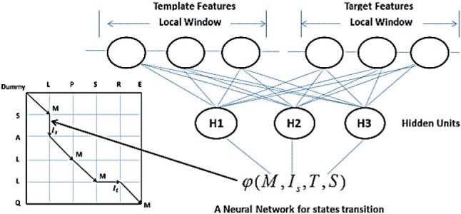
An example of the edge feature function φ, which is a neural network with one hidden layer. The function takes both template and target protein features as input and yields one log-likelihood score for state transition M to Is. Meanwhile, H1, H2 and H3 are hidden neurons conducting non-linear transformation of the input features
Because a hidden layer is introduced in the CNF to improve its expressive power over a CRF, it is important to control the model complexity to avoid overfitting. We do so by using a L2-norm regularization factor, which is determined by 5-fold cross-validation, to restrict the search space of model parameters. Once the CNF model is trained, we can calculate the optimal alignment using the Viterbi algorithm (Viterbi, 1967).
2.2 Training CNF models by the quality-sensitive method
CRFs and CNFs are usually trained by ML or maximum a posteriori (MAP) (Volkovs and Zemel, 2009) methods. The ML method trains the CRF or CNF model parameters by maximizing the observed probability of a set of reference alignments built by a structure alignment tool. The ML method treats all of the aligned positions equally, ignoring the fact that some are more conserved than others. It is important not to misalign the conserved residues since they may be related to protein function. As such, it makes more sense to treat conserved and non-conserved residues differently. Although there are several measures for the degree of conservation to be studied, here we simply use the local TM-score (Zhang and Skolnick, 2004) between two aligned residues. Given a reference alignment (and the superimposition of two proteins in the alignment), the local TM-score at one alignment position i is defined as follows:
| (4) |
where di is the distance deviation between the two aligned residues at position i and d0 is a normalization constant depending only on protein length. The TM-score ranges from 0 to 1, with higher values indicating more highly conserved aligned positions. When the alignment state at position i is a gap, the local TM-score is equal to 0. That is, wi is equal to 0.
To differentiate the degree of conservation among positions in the alignment, we train the CNF model by maximizing the expected TM-score. The expected TM-score of one threading alignment is defined as follows:
| (5) |
where N(A) is the smaller length of the two proteins and MAGi is the marginal alignment probability at alignment position i. Since wi is equal to 0 at a gap position, Equation (5) sums the marginal alignment probabilities over all the alignment positions with the match state (i.e. state M). Given two residues of a pair of proteins, the marginal alignment probability is equal to the accumulative probability of all possible alignments of this pair of proteins in which these two residues are aligned to each other. The marginal alignment probability can be calculated efficiently using the forward–backward algorithm (Lafferty et al., 2001). See the Supplementary Material for more technical details. Equation (5) is similar to the definition of TM-score except that the latter does not have a term for the marginal alignment probability. By maximizing Equation (5), we place greater weight on the aligned residue pairs with higher local TM-score (that is, more conserved residue pairs) instead of treating all of the aligned residue pairs equally. We term this approach a quality-sensitive training method.
The expected TM-score in Equation (5) is not concave, so it is challenging to optimize to its global optimum. Here we use the L-BFGS [Limited memory BFGS (Liu and Nocedal, 1989)] algorithm to solve it suboptimally. To obtain a good solution, we run L-BFGS several times starting from different initial solutions and return the best suboptimal solution. In order to use the L-BFGS algorithm, we need to calculate the gradient of Equation (5), which is detailed in the Supplementary Material.
2.3 Protein features
We generate a position-specific score matrix (PSSM) for a template and a position-specific frequency matrix (PSFM) for a target using PSI-BLAST (Altschul et al., 1997) with five iterations and an E-value of 0.001. Let PSSM(i,aa) denote the mutation potential for amino acid aa at template position i and PSFM(j,aa) the observed frequency of amino acid aa at target position j.
2.3.1 Features for a match state
We use the following features to estimate the alignment probability of two residues:
Sequence profile similarity: the profile similarity between two positions is calculated by ∑PSSM(i, a)PSFM(i, a). We also calculate sequence similarity using the Gonnet matrix (Gonnet et al., 1992) and BLOSUM62 (Henikoff and Henikoff, 1992).
Amino acid substitution matrix: we use two matrices. One is the matrix developed by the Kihara group (Tan et al., 2006) and the other is a structure-based substitution matrix. Each entry in Kihara's matrix measures the similarity between two amino acids using the correlation coefficient of their contact potential vectors. The contact potential vector of each amino acid contains 20 elements, each of which indicates the contact potential with one of the 20 amino acids. The structure-based substitution matrix (Prli et al., 2000; Tan et al., 2006) is more sensitive than BLOSUM (Henikoff and Henikoff, 1992) for the alignment of distantly related proteins.
Secondary structure score: we evaluate the secondary structure similarity between the target and template in terms of both the 3-class and 8-class types. We generate secondary structure types for the template using DSSP (Kabsch and Sander, 1983). We also predict the 3-class and 8-class secondary structure types for the target using PSIPRED (McGuffin et al., 2000) and our in-house tool RaptorX-SS8 (Wang et al., 2010), respectively.
Solvent accessibility score: we discretize the solvent accessibility into three equal-frequency states: buried, intermediate and exposed. The equal-frequency method is the best among several discretization methods we tested. We use our in-house tool to predict the solvent accessibility of the target, and DSSP (Kabsch and Sander, 1983) to calculate the solvent accessibility of the template. Let sa denote the solvent accessibility type on the template. The solvent accessibility similarity is defined as the predicted likelihood of the target residue being in sa.
Environment fitness score: this score measures how well one sequence residue aligns to a specific template environment. We define the environment of a template residue as the combination of its solvent accessibility state and 3-class secondary structure type, which results in nine environment types.
Neighborhood similarity score: Pei and Grishin (2001) showed that conserved positions tend to cluster together along the sequence. That is, if two residues can be aligned, it is likely that the residues around them can also be aligned. Therefore, we can use the neighborhood information to estimate the likelihood of two residues being aligned. The neighborhood information used in our model includes sequence profile, secondary structure, and solvent accessibility, in a window of size 11.
Residues in two terminals: residues at the two terminals may not have sufficient neighborhood information, and thus need some special handling. We use one binary variable to indicate if a residue is at a terminal position or not.
Disordered regions: disordered regions are natively unfolded or intrinsically unstructured, lacking stable tertiary structure (Marcin et al., 2011). Therefore, we do not use structure information (namely, secondary structure or solvent accessibility) to determine the alignment of disordered regions, because it might introduce more false positives. We use DISOPRED (Ward et al., 2004) to predict disordered regions in a sequence, which produces a confidence score, ranging from 0 to 9, to indicate how likely a residue is to be in a disordered region. A higher confidence score indicates a greater likelihood of a residue being in a disordered region. We deem a residue to be in a disordered region if the confidence score is 9. When aligning disordered residues, only sequence information is used and all the predicted structure information is ignored; that is, their relevant feature values are set to 0.
2.3.2 Features for a gap state
Unlike many sequence alignment programs (Altschul et al., 1997; Mott, 2005), CNFpred does not use an affine gap penalty. Instead, it uses both position-specific and context-specific features to estimate a gap probability. We derive the position-specific features from the alignment of the sequence homologs of a given protein while the context-specific features include amino acid identify, hydropathy index, both 3-class and 8-class secondary structure, and solvent accessibility. We also differentiate a gap in either end of a protein from that in the middle of a protein.
3 RESULTS
3.1 Training data
We constructed the training and validation data from PDB25, downloaded from PISCES (Wang and Dunbrack, 2003). Any two proteins in PDB25 share <25% sequence identity. We used a set of 1010 protein pairs extracted from PDB25, which covers most of the SCOP fold classes, as the training data. We used another set of 200 protein pairs from PDB25 as the validation data. There is no redundancy between the training and validation data (there was no overlap, and this dataset ensures <25% sequence identity). The reference structure alignments for the training and validation data are built using our in-house structure alignment tool DeepAlign.
3.2 Test data
We use the following four test sets.
In-house benchmark. This benchmark set consists of 3600 protein pairs drawn from PDB25. This set has no redundancy with the training and validation data (that is, all proteins share <25% sequence identity). It is constructed so that (i) it contains representatives from all protein classes (α, β and α–β proteins); (ii) the protein NEFF values are nearly uniformly distributed; (iii) the protein lengths are widely distributed; and (iv) TM-scores of all the pairs are spread out between 0.5 and 0.7.
MUSTER benchmark (Wu and Zhang, 2008). This set contains all the training data used by the MUSTER threading program, consisting of 110 hard ProSup pairs and another 190 pairs selected by the Zhang group, each pair having TM-score >0.5.
SALIGN benchmark (Marti Renom et al., 2004). This set contains 200 protein pairs, each of which shares ~20% sequence identity and ~65% structurally equivalent residues with RMSD <3.5Å. Many protein pairs in this set contain proteins of very different size, which makes it very challenging for any threading methods.
ProSup benchmark (Lackner et al., 2000). This set consists of 127 protein pairs.
3.3 Programs to compare
We compare our CNF threading method, CNFpred, with the top-notch profile-based and threading methods such as HHpred (Söding et al., 2005), MUSTER (Wu and Zhang, 2008), SPARKS/SP3/SP5 (Zhou and Zhou, 2005), SALIGN (Marti Renom et al., 2004), RAPTOR (Xu et al., 2003) and BThreader (Peng and Xu, 2009). We use the published results for SPARKS/SP3/SP5 since they have their own template file formats and we cannot correctly run them locally. We use the published result for SALIGN since it is unavailable. We focus on comparing CNFpred with HHpred and BThreader since the latter two performed extremely well in the most recent CASP competition in 2010.
3.4 Evaluation criteria
We evaluate the threading methods using both reference-dependent and reference-independent alignment accuracy. The reference-dependent accuracy is defined as the percentage of correctly aligned positions judged by the reference alignments. For all benchmarks, we use four structure alignment tools to generate reference alignments: TM-align (Zhang and Skolnick, 2005), Matt (Menke et al., 2008), Dali (Holm and Sander, 1993) and our in-house structure alignment tool DeepAlign. In addition, the ProSup and MUSTER benchmarks have their own reference alignments. To avoid bias toward a specific structure alignment tool, we evaluate threading alignment accuracy using all the reference alignments mentioned above. Note that CNFpred is trained using only the structure alignments generated by our in-house tool DeepAlign. To evaluate the reference-independent alignment accuracy, we build a 3D model for the target protein using MODELLER (Šali et al., 1995) from its alignment to the template and then evaluate the quality of the resulting 3D model using TM-score. TM-score ranges from 0 to 1, indicating the worst and best model quality, respectively.
3.5 Reference-dependent alignment accuracy
As shown in Tables 1–4, CNFpred outperforms all others, regardless of the reference alignments used. The advantage of CNFpred over the popular profile-profile alignment method HHpred increases with respect the hardness of the benchmark. For example, on the most challenging In-House benchmark the relative improvement of CNFpred over HHpred is >20%. Even on the easiest ProSup benchmark the relative improvement of CNFpred over HHpred is ~10%. Our old threading program, BThreader, works well on the ProSup and SALIGN sets, but not as well on the MUSTER or In-house benchmarks. On these two benchmarks, BThreader has similar performance to HHpred (global alignment), but much worse than CNFpred. CNFpred has a smaller advantage over the others on the SALIGN benchmark. This is because this benchmark contains many proteins with symmetric domains, which have several good alternative structure alignments. However, we only use the first alignment generated by the structure alignment tools for a protein pair as the reference alignment. Therefore, even if the threading alignments are pretty good, they may still have very low accuracy when judged by the ‘imperfect’ reference alignments.
Table 1.
Reference-dependent alignment accuracy on the In-House benchmark
| Methods | TMalign | Dali | Matt | DeepAlign |
|---|---|---|---|---|
| HHpred(Local) | 32.63 | 36.60 | 35.53 | 35.47 |
| HHpred(Global) | 38.80 | 43.65 | 42.48 | 42.78 |
| BThreader | 37.44 | 41.85 | 40.17 | 40.95 |
| CNFpred | 46.49 | 51.77 | 49.98 | 51.19 |
Columns 2–5 indicate four different tools generating the reference alignments. Bold indicates the best performance.
Table 2.
Reference-dependent alignment accuracy on the MUSTER benchmark
| Methods | TMalign | Dali | Matt | DeepAlign | BR |
|---|---|---|---|---|---|
| HHpred(Local) | 42.96 | 57.34 | 46.00 | 46.50 | 45.34 |
| HHpred(Global) | 48.82 | 53.13 | 51.48 | 52.48 | 51.48 |
| MUSTER | – | – | – | – | 46.70 |
| BThreader | 47.35 | 51.30 | 50.13 | 50.53 | 50.01 |
| CNFpred | 54.17 | 58.46 | 57.26 | 59.14 | 57.06 |
Columns 2–5 indicate four different tools generating the reference alignments. Column ‘BR’ indicates the reference alignments provided in the benchmark. The result for MUSTER is the training accuracy taken from Wu and Zhang (2008). All other numbers are test accuracy. Bold indicates the best performance.
Table 3.
Reference-dependent alignment accuracy on the SALIGN benchmark
| Methods | TMalign | Dali | Matt | DeepAlign |
|---|---|---|---|---|
| SPARKS | 53.10 | – | – | – |
| SALIGN | 56.40 | – | – | – |
| RAPTOR | 40.00 | – | – | – |
| SP3 | 56.30 | – | – | – |
| SP5 | 59.70 | – | – | – |
| HHpred(Local) | 60.64 | 62.94 | 62.97 | 63.16 |
| HHpred(Global) | 62.98 | 63.14 | 63.87 | 63.53 |
| BThreader | 64.40 | 63.13 | 63.05 | 64.09 |
| CNFpred | 66.73 | 67.95 | 68.17 | 69.50 |
The results for SALIGN and RAPTOR are taken from (Qiu and Elber, 2006) and from (Xu, 2005), respectively. The results for SPARKS, SP3 and SP5 are taken from Zhang et al. (2008). Bold indicates the best performance. Columns 2–5 correspond to four different tools generating reference alignments.
Table 4.
Reference-dependent alignment accuracy on the ProSup benchmark
| Methods | TMalign | Dali | Matt | DeepAlign | BR |
|---|---|---|---|---|---|
| SPARKS | – | – | – | – | 57.2 |
| SALIGN | – | – | – | – | 58.3 |
| RAPTOR | – | – | – | – | 61.3 |
| SP3 | – | – | – | – | 65.3 |
| SP5 | – | – | – | – | 68.7 |
| HHpred(Local) | 57.53 | 60.58 | 60.61 | 60.36 | 64.90 |
| HHpred(Global) | 61.84 | 65.31 | 64.52 | 65.29 | 69.04 |
| BThreader | 60.87 | 64.89 | 63.97 | 64.26 | 76.08 |
| CNFpred | 66.26 | 71.16 | 71.06 | 72.01 | 77.09 |
Columns 2–5 correspond to four different tools generating reference alignments. Column ‘BR’ denotes the reference alignments provided in the benchmark. The results of SPARKS, SP3 and SP5, of SALIGN and of RAPTOR are taken form Zhang et al. (2008), from Qiu and Elber (2006) and from Xu (2005), respectively. Bold indicates the best performance.
3.6 Reference-independent alignment accuracy
Tested on the much more challenging In-House benchmark, CNFpred obtains a TM-score of 1693, which is >10% improvement when compared with HHpred and BThreader. In addition, on SALIGN and Prosup, CNFpred obtains accumulative TM-scores of 134.5 and 67.34, respectively. In contrast, HHpred has TM-scores of 121.83 and 56.44, respectively, as shown in Table 5.
Table 5.
Reference-independent alignment accuracy, measured by TM-score, on the four benchmarks: In-House, MUSTER, SALIGN and ProSup
| Methods | In-House | MUSTER | SALIGN | ProSup |
|---|---|---|---|---|
| HHpredL | 1047.56 | 108.84 | 119.97 | 53.88 |
| HHpredG | 1522.77 | 142.00 | 121.83 | 56.44 |
| MUSTER | – | 136.47 | – | – |
| BThreader | 1537.89 | 143.95 | 132.85 | 66.77 |
| CNFpred | 1692.17 | 152.14 | 134.50 | 67.34 |
The result for MUSTER is its training accuracy (Wu and Zhang, 2008). All the other results are test accuracy. Bold indicates the best performance.
3.7 Alignment accuracy with respect to sparsity of sequence profile
To further examine the performance of CNFpred, BThreader and HHpred with respect to the level of homologous information, we divide the protein pairs in the In-House benchmark into nine groups according to the minimum NEFF value of a protein pair and calculate the average TM-score of the target models in each group. As shown in Figure 3A, when NEFF is small (that is, proteins have sparse sequence profiles), our method outperforms BThreader and HHpred significantly. We also divide all the protein pairs in the benchmark into four groups according to the NEFF values of the proteins in each pair using a threshold of 6. As shown in Figure 3B, when the NEFF values of both proteins in a pair are small (<6), our method is 33% better than HHpred. When only one of the two proteins in a pair has NEFF <6, our method is 25% better than HHpred. Even when both proteins in a pair have NEFF values >6, which indicates both proteins have sufficient homologous information, our method still outperforms HHpred slightly. In summary, CNFpred excels for proteins with sparse sequence profiles.
Fig. 3.
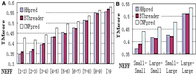
Reference-independent alignment accuracy with respect to the sparsity of a sequence profile (i.e. NEFF). (A) NEFF is divided into nine bins. (B) NEFF is divided into two bins at the threshold 6
3.8 Alignment accuracy with respect to protein classes and lengths
As shown in Figure 4, CNFpred is superior to others across all protein classes and lengths. CNFpred performs especially well for all-β proteins because it makes better use of structure information.
Fig. 4.

(A) Reference-independent alignment accuracy with respect to (A) protein class and (B) protein length. A protein with <150 amino acids is treated as small; otherwise as large
3.9 Threading performance with different features
Table 6 shows the alignment quality, measured by TM-score, when different protein features are used. All the CNF models are trained on the same set of training data, regardless of features, and are tested on our in-house benchmark. This benchmark is challenging, which enables us to more easily demonstrate the contribution of different protein features and the impact of different training approaches. For ML and quality-sensitive training, the Viterbi algorithm is used to generate alignments. For MAP the Maximum Expected Accuracy (MEA) algorithm (Biegert and Söding, 2008) is used to generate alignments. We treat sequence profiles and 3-class secondary structure as the basis features and then evaluate the value added by the 8-class secondary structure and 3-class solvent accessibility. As shown in Table 6, the 8-class secondary structure and 3-class solvent accessibility improve the alignment accuracy by 0.01 and 0.02, respectively, regardless of the training approach. Meanwhile, predicted solvent accessibility improves the alignment accuracy the most. The MAP training method improves the accuracy by 0.01 over the ML method while the quality-sensitive training method improves the accuracy by 0.01 over the MAP method. The quality-sensitive method significantly improves the overall performance.
Table 6.
The contribution of protein features and the impact of different training methods
| Training approaches | ML | MAP | Quality-sensitive |
|---|---|---|---|
| Profile + SS3 | 1536.01 | 1578.60 | 1612.44 |
| Profile + SS3 + SS8 | 1567.81 | 1595.72 | 1637.64 |
| Profile + SS3 + SA | 1606.68 | 1616.04 | 1662.12 |
| Profile + SS3 + SS8 + SA | 1633.32 | 1664.28 | 1692.17 |
The results are obtained on our In-House benchmark. SS3 and SS8 indicate the 3-class and 8-class secondary structure, respectively. SA indicates the 3-class solvent accessibility.
3.10 Threading performance on a large set
We construct a fairly large set from PDB25 as follows. All of the ~6000 proteins in PDB25 are used as templates and 1000 of them are randomly chosen as the target set. We run CNFpred and HHpred to predict the 3D structure for each of the 1000 targets using all of the ~6000 templates. When predicting structure for one specific target protein, the target itself is removed from the template list. We run HHpred using the ‘realign’ option. That is, for a given target, HHpred first searches through all templates using local alignment, and then realigns the target to its top templates using global alignment. We use the default values for the other HHpred parameters. CNFpred first generates target–template alignments and then ranks the templates using a neural network, which predicts the quality (TM-score) of an alignment. The template with the best predicted alignment quality is then used to build a 3D model for the target. As shown in Figure 5A, CNFpred performs significantly better than HHpred when the targets are difficult (that is, when the HHpred model has a TM-score <0.7). On the 1000 targets, CNFpred and HHpred obtain overall TM-scores of 558 and 515, respectively. If we exclude the 170 ‘easy’ targets (those for which, either CNFpred or HHpred model has a TM-score >0.8) from consideration, the overall TM-scores obtained by CNFpred and HHpred are 416 and 375, respectively. In other words, CNFpred is ~10.9% better than HHpred. As shown in Figure 5B, CNFpred generates models better than HHpred by at least 0.05 TM-score on 329 targets while HHpred is better than CNFpred by this margin on only 76 targets. Furthermore, CNFpred generates models better than HHpred by at least 0.10 TM-score on 192 targets, while HHpred is better than CNFpred by this margin on only 27 targets. In summary, CNFpred has a significant advantage over HHpred on the hard targets.
Fig. 5.

(A) TM-scores of the CNFpred and HHpred models for the 1000 targets from PDB25. Each point represents two models, one generated by CNFpred, and one by HHpred. (B) Distribution of the TM-score difference of two 3D models for the same target. Each blue (red) column shows the number of targets for which CNFpred (HHpred) is better by a given margin
4 CONCLUSION
We have presented CNFpred, a novel CNF model for threading of proteins with sparse sequence profiles. CNFpred takes advantage of as many correlated sequence and structure features as possible to improve alignment accuracy. We have also presented a quality-sensitive training method to improve alignment accuracy, as opposed to the standard ML method. Despite using many features and a non-linear scoring function, CNFpred can still efficiently generate optimal alignments via dynamic programming. It takes only seconds to thread a typical protein pair. Experimental results demonstrate that our CNFpred outperforms the CASP-winning programs, regardless of benchmarks, reference alignments, protein classes or protein lengths. Currently, CNFpred only considers state transitions between two adjacent positions. We can also model pairwise interaction between two non-adjacent positions, but training such a model is computationally challenging, perhaps requiring us to resort to approximation algorithms.
Homologous information is very effective in detecting remote homologs, as evidenced by the profile-based method HHpred, which outperformed many threading methods in recent CASP events. This article shows that homologous information is not sufficient for proteins with sparse sequence profiles (low NEFF) and that we can improve alignment accuracy over profile-based methods by using more structure information, especially for proteins with sparse sequence profiles. The Cowen group takes a rather different approach, called simulated evolution, to enrich sequence profiles, and shows that the alignment accuracy can be improved for some proteins (Kumar and Cowen, 2009). The ability to predict structures for proteins with sparse sequence profiles is very important. Simple statistics indicate that among the ~6877 Pfam families (Bateman et al., 2004) without solved structures, 79.2, 63.7, 45.5 and 25.4% have NEFF ≤6, 5, 4 and 3, respectively, and of the 5332 Pfam families with solved structures, ~57% have NEFF <6. In addition, ~25% of the protein sequences in UniProt (Bairoch et al., 2005) are not covered by Pfam (ver 25.0). A significant number of these sequences are singletons (i.e. products of orphan genes) and, thus, have NEFF = 1. In the foreseeable future, we expect that there will be a lack of solved structures for many low-homology proteins and families (NEFF ≤6). Therefore, our CNF threading method will be useful for a large percentage of protein sequences without solved structures.
Supplementary Material
ACKNOWLEDGEMENTS
The authors are grateful to the University of Chicago Beagle team, TeraGrid and Canadian SHARCNet for their support of computational resources.
Funding: National Institutes of Health [R01GM0897532], National Science Foundation [DBI-0960390] and Microsoft PhD Research Fellowship.
Conflict of Interest: none declared.
REFERENCES
- Akutsu T., et al. Hardness results on local multiple alignment of biological sequences. Inform. Media Technol. 2007;2:514–522. [Google Scholar]
- Altschul S.F., et al. Gapped BLAST and PSI-BLAST: a new generation of protein database search programs. Nucleic Acids Res. 1997;25:3389–3402. doi: 10.1093/nar/25.17.3389. [DOI] [PMC free article] [PubMed] [Google Scholar]
- Bairoch A., et al. The universal protein resource (UniProt) Nucleic Acids Res. 2005;33:D154–D159. doi: 10.1093/nar/gki070. [DOI] [PMC free article] [PubMed] [Google Scholar]
- Bateman A., et al. The Pfam protein families database. Nucleic Acids Res. 2004;32:D138–D141. doi: 10.1093/nar/gkh121. [DOI] [PMC free article] [PubMed] [Google Scholar]
- Biegert A., Söding J. De novo identification of highly diverged protein repeats by probabilistic consistency. Bioinformatics. 2008;24:807–814. doi: 10.1093/bioinformatics/btn039. [DOI] [PubMed] [Google Scholar]
- Biegert A., Söding J. Sequence context-specific profiles for homology searching. Proc. Natl Acad. Sci. USA. 2009;106:3770–3775. doi: 10.1073/pnas.0810767106. [DOI] [PMC free article] [PubMed] [Google Scholar]
- Cozzetto D., Tramontano A. Relationship between multiple sequence alignments and quality of protein comparative models. Prot. Struct. Funct. Bioinformatics. 2005;58:151–157. doi: 10.1002/prot.20284. [DOI] [PubMed] [Google Scholar]
- Do C.B., Brudno M., Batzoglou S. Prob Cons: Probabilistic Consistency-Based Multiple Alignment of Amino Acid Sequences. AAAI Press; 2004. pp. 703–708. MIT Press, Menlo Park, CA; Cambridge, MA; London. [Google Scholar]
- Eskin E., Snir S. Incorporating homologues into sequence embeddings for protein analysis. J. Bioinformatics Comput. Biol. 2007;5:717–738. doi: 10.1142/s0219720007002734. [DOI] [PubMed] [Google Scholar]
- Gonnet G.H., Cohen M.A., Benner S.A. Exhaustive matching of the entire protein sequence database. Science. 1992;256:1443. doi: 10.1126/science.1604319. [DOI] [PubMed] [Google Scholar]
- Haykin S. Neural Networks: A Comprehensive Foundation. Prentice Hall; 1999. http://www.pearsonhighered.com/academic/product?ISBN=0132733501. [Google Scholar]
- Henikoff S., Henikoff J.G. Amino acid substitution matrices from protein blocks. Proc. Natl Acad. Sci. USA. 1992;89:10915. doi: 10.1073/pnas.89.22.10915. [DOI] [PMC free article] [PubMed] [Google Scholar]
- Hildebrand A., et al. Fast and accurate automatic structure prediction with HHpred. Prot. Struct. Funct. Bioinformatics. 2009;77:128–132. doi: 10.1002/prot.22499. [DOI] [PubMed] [Google Scholar]
- Holm L., Sander C. Protein structure comparison by alignment of distance matrices. J. Mol. Biol. 1993;233:123–123. doi: 10.1006/jmbi.1993.1489. [DOI] [PubMed] [Google Scholar]
- Itoh M., et al. Clustering of database sequences for fast homology search using upper bounds on alignment score. Genome Inform. 2004;15:93–104. [PubMed] [Google Scholar]
- Jaroszewski L., et al. FFAS03: a server for profile–profile sequence alignments. Nucleic Acids Res. 2005;33:W284–W288. doi: 10.1093/nar/gki418. [DOI] [PMC free article] [PubMed] [Google Scholar]
- Jones D.T. GenTHREADER: an efficient and reliable protein fold recognition method for genomic sequences1. J. Mol. Biol. 1999;287:797–815. doi: 10.1006/jmbi.1999.2583. [DOI] [PubMed] [Google Scholar]
- Kabsch W., Sander C. Dictionary of protein secondary structure: pattern recognition of hydrogen-bonded and geometrical features. Biopolymers. 1983;22:2577–2637. doi: 10.1002/bip.360221211. [DOI] [PubMed] [Google Scholar]
- Karplus K., et al. Hidden Markov models for detecting remote protein homologies. Bioinformatics. 1998;14:846–856. doi: 10.1093/bioinformatics/14.10.846. [DOI] [PubMed] [Google Scholar]
- Kelley L.A., et al. Enhanced genome annotation using structural profiles in the program 3D-PSSM1. J. Mol. Biol. 2000;299:501–522. doi: 10.1006/jmbi.2000.3741. [DOI] [PubMed] [Google Scholar]
- Kumar A., Cowen L. Augmented training of hidden Markov models to recognize remote homologs via simulated evolution. Bioinformatics. 2009;25:1602. doi: 10.1093/bioinformatics/btp265. [DOI] [PMC free article] [PubMed] [Google Scholar]
- Lackner P., et al. ProSup: a refined tool for protein structure alignment. Prot. Engineer. 2000;13:745. doi: 10.1093/protein/13.11.745. [DOI] [PubMed] [Google Scholar]
- Lafferty J., et al. Conditional Random Fields: Probabilistic Models for Segmenting and Labeling Sequence Data. San Francisco, CA, USA: Morgan Kaufmann Publishers Inc.; 2001. pp. 282–289. [Google Scholar]
- Liu D.C., Nocedal J. On the limited memory BFGS method for large scale optimization. Math. Program. 1989;45:503–528. [Google Scholar]
- Marcin M., et al. In-silico prediction of disorder content using hybrid sequence representation. 2011 doi: 10.1186/1471-2105-12-245. [DOI] [PMC free article] [PubMed] [Google Scholar]
- Marti Renom M.A., et al. Alignment of protein sequences by their profiles. Protein Sci. 2004;13:1071–1087. doi: 10.1110/ps.03379804. [DOI] [PMC free article] [PubMed] [Google Scholar]
- McGuffin L.J., et al. The PSIPRED protein structure prediction server. Bioinformatics. 2000;16:404. doi: 10.1093/bioinformatics/16.4.404. [DOI] [PubMed] [Google Scholar]
- Meng L., et al. Sequence alignment as hypothesis testing. J. Comput. Biol. 2011;18:677–691. doi: 10.1089/cmb.2010.0328. [DOI] [PMC free article] [PubMed] [Google Scholar]
- Menke M., et al. Matt: local flexibility aids protein multiple structure alignment. PLoS Comput. Biol. 2008;4:e10. doi: 10.1371/journal.pcbi.0040010. [DOI] [PMC free article] [PubMed] [Google Scholar]
- Mott R. Smith–Waterman Algorithm. 2005 eLS. Please see http://onlinelibrary.wiley.com/doi/10.1038/npg.els.0005263/abstractfor more information. [Google Scholar]
- O'Rourke S., et al. Discrete profile alignment via constrained information bottleneck. Adv. Neural Inform. Processing Sys. 2005;17:1009–1016. [Google Scholar]
- Pei J., Grishin N.V. AL2CO: calculation of positional conservation in a protein sequence alignment. Bioinformatics. 2001;17:700. doi: 10.1093/bioinformatics/17.8.700. [DOI] [PubMed] [Google Scholar]
- Peng J., et al. Conditional neural fields. Adv. Neural Informat. Process. Syst. 2009;22:1419–1427. [Google Scholar]
- Peng J., Xu J. Proceedings of the 13th Annual International Conference on Research in Computational Molecular Biology. Tucson, Arizona: Springer-Verlag; 2009. Boosting Protein Threading Accuracy; pp. 31–45. [DOI] [PMC free article] [PubMed] [Google Scholar]
- Prli A., et al. Structure-derived substitution matrices for alignment of distantly related sequences. Prot. Engineer. 2000;13:545. doi: 10.1093/protein/13.8.545. [DOI] [PubMed] [Google Scholar]
- Qiu J., Elber R. SSALN: an alignment algorithm using structure dependent substitution matrices and gap penalties learned from structurally aligned protein pairs. Prot. Struct. Funct. Bioinformatics. 2006;62:881–891. doi: 10.1002/prot.20854. [DOI] [PubMed] [Google Scholar]
- Söding J., et al. The HHpred interactive server for protein homology detection and structure prediction. Nucleic Acids Res. 2005;33:W244. doi: 10.1093/nar/gki408. [DOI] [PMC free article] [PubMed] [Google Scholar]
- Šali A., et al. Evaluation of comparative protein modeling by MODELLER. Prot. Struct. Funct. Bioinformatics. 1995;23:318–326. doi: 10.1002/prot.340230306. [DOI] [PubMed] [Google Scholar]
- Schönhuth A., et al. Pair HMM based gap statistics for re-evaluation of indels in alignments with affine gap penalties. Proceedings of the WABI2010. 2010:350–361. LNCS 6293. [Google Scholar]
- Shi J., et al. FUGUE: sequence-structure homology recognition using environment-specific substitution tables and structure-dependent gap penalties1. J. Mol. Biol. 2001;310:243–257. doi: 10.1006/jmbi.2001.4762. [DOI] [PubMed] [Google Scholar]
- Sommer I., et al. Improving the quality of protein structure models by selecting from alignment alternatives. BMC Bioinformatics. 2006;7:364. doi: 10.1186/1471-2105-7-364. [DOI] [PMC free article] [PubMed] [Google Scholar]
- Tan Y.H., et al. Statistical potential based amino acid similarity matrices for aligning distantly related protein sequences. Prot. Struct. Funct. Bioinformatics. 2006;64:587–600. doi: 10.1002/prot.21020. [DOI] [PubMed] [Google Scholar]
- Viterbi A. Error bounds for convolutional codes and an asymptotically optimum decoding algorithm. Inform. Theory IEEE Transact. 1967;13:260–269. [Google Scholar]
- Volkovs M.N., Zemel R.S. Proceedings of the 26th Annual International Conference on Machine Learning. Montreal, Quebec, Canada: ACM; 2009. BoltzRank: Learning to Maximize Expected Ranking Gain; pp. 1089–1096. [Google Scholar]
- Waldispühl J., et al. Proceedings of the 13th Annual International Conference on Research in Computational Molecular Biology. Tucson, Arizona: Springer-Verlag; 2009. Simultaneous alignment and folding of protein sequences; pp. 339–355. [Google Scholar]
- Wang G., Dunbrack R.L. PISCES: a protein sequence culling server. Bioinformatics. 2003;19:1589. doi: 10.1093/bioinformatics/btg224. [DOI] [PubMed] [Google Scholar]
- Wang Z., et al. Protein 8-class secondary structure prediction using Conditional Neural Fields. IEEE. 2010:109–114. doi: 10.1002/pmic.201100196. [DOI] [PMC free article] [PubMed] [Google Scholar]
- Ward J.J., et al. The DISOPRED server for the prediction of protein disorder. Bioinformatics. 2004;20:2138. doi: 10.1093/bioinformatics/bth195. [DOI] [PubMed] [Google Scholar]
- Wu S., Zhang Y. MUSTER: improving protein sequence profile–profile alignments by using multiple sources of structure information. Prot. Struct. Funct. Bioinformatics. 2008;72:547–556. doi: 10.1002/prot.21945. [DOI] [PMC free article] [PubMed] [Google Scholar]
- Xu J. Fold recognition by predicted alignment accuracy. IEEE/ACM Trans. Computat. Biol. Bioinformatics. 2005;2:157–165. doi: 10.1109/TCBB.2005.24. [DOI] [PubMed] [Google Scholar]
- Xu J., et al. RAPTOR: optimal protein threading by linear programming. Int. J. Bioinform. Comput. Biol. 2003;1:95–118. doi: 10.1142/s0219720003000186. [DOI] [PubMed] [Google Scholar]
- Zhang Y., Skolnick J. Scoring function for automated assessment of protein structure template quality. Prot. Struct. Funct. Bioinformatics. 2004;57:702–710. doi: 10.1002/prot.20264. [DOI] [PubMed] [Google Scholar]
- Zhang Y., Skolnick J. TM-align: a protein structure alignment algorithm based on the TM-score. Nucleic Acids Res. 2005;33:2302. doi: 10.1093/nar/gki524. [DOI] [PMC free article] [PubMed] [Google Scholar]
- Zhang W., et al. SP5: improving protein fold recognition by using torsion angle profiles and profile-based gap penalty model. PLoS One. 2008;3:e2325. doi: 10.1371/journal.pone.0002325. [DOI] [PMC free article] [PubMed] [Google Scholar]
- Zhao F., et al. Fragment-free approach to protein folding using conditional neural fields. Bioinformatics. 2010;26:i310. doi: 10.1093/bioinformatics/btq193. [DOI] [PMC free article] [PubMed] [Google Scholar]
- Zhou H., Zhou Y. SPARKS 2 and SP3 servers in CASP6. Prot. Struct. Funct. Bioinformatics. 2005;61:152–156. doi: 10.1002/prot.20732. [DOI] [PubMed] [Google Scholar]
Associated Data
This section collects any data citations, data availability statements, or supplementary materials included in this article.