Spatial resolution properties of motion-compensated tomographic image reconstruction methods

Abstract

Many motion-compensated image reconstruction (MCIR) methods have been proposed to correct for subject motion in medical imaging. MCIR methods incorporate motion models to improve image quality by reducing motion artifacts and noise.

This paper analyzes the spatial resolution properties of MCIR methods and shows that nonrigid local motion can lead to non-uniform and anisotropic spatial resolution for conventional quadratic regularizers. This undesirable property is akin to the known effects of interactions between heteroscedastic log-likelihoods (e.g., Poisson likelihood) and quadratic regularizers. This effect may lead to quantification errors in small or narrow structures (such as small lesions or rings) of reconstructed images.

This paper proposes novel spatial regularization design methods for three different MCIR methods that account for known nonrigid motion. We develop MCIR regularization designs that provide approximately uniform and isotropic spatial resolution and that match a user-specified target spatial resolution. 2D PET simulations demonstrate the performance and benefits of the proposed spatial regularization design methods.

I. Introduction

MOTION can degrade image quality in medical imaging. Often medical imaging systems cannot capture ideal quality images due to their innate acquisition speeds and patient motion. Gating methods have been investigated to reduce motion artifacts [1], [2], but can suffer from insufficient measurements that result in low signal-to-noise ratio (SNR) images. Motion-compensated image reconstruction (MCIR) methods have been studied for various imaging modalities to improve image quality by using all collected data and motion information so that high SNR images are reconstructed without motion artifacts [3]–[16].

MCIR methods differ in terms of how they incorporate motion information. We focus here on three common MCIR methods: post-reconstruction motion correction (PMC) [3]–[5], motion-compensated temporal regularization (MTR) [6], [7], and the parametric motion model (PMM) [8]–[16] (see Table I). These models have also been used in non-medical super-resolution applications [17]–[20]. These MCIR methods have shown promising results for reducing noise and motion artifacts. MCIR methods have great potential for improving image quality and benefiting the tasks used in medical imaging (e.g., better quantitative accuracy for PET or lower radiation dose for CT).

TABLE I.

Acronyms

Acronym
MCIR	motion-compensated image reconstruction
LIR	local impulse response

Acronym	Reconstruction method
SGR	single gated reconstruction
PMC	post-reconstruction motion correction
MTR	motion-compensated temporal regularization
PMM	the parametric motion model

Acronym	Regularization method
-S	standard quadratic regularizer
-C	certainty-based regularizer
-P	proposed regularizer

The interactions between heteroscedastic log-likelihood models (e.g., Poisson measurements) and conventional static quadratic regularizers lead to non-uniform and anisotropic spatial resolution [21]. In this paper, we show analytically that these undesired properties can become worse in regularized MCIR methods due to local motion, may cause non-uniform and anisotropic spatial resolution, and produce quantification errors in small or narrow structures such as small lesions or rings of reconstructed images. For example, Fig. 1 shows the contours of local impulse response (LIR) functions of Target (desired LIR), SGR-S (single gated reconstruction with conventional spatial regularizer using one frame), and PMC-S (PMC with conventional static spatial regularizer using four frames) in a 2D PET simulation (see Table I for acronyms). Each LIR was generated by subtracting the reconstructed image of the noiseless projection data of the original image from the reconstructed image of the noiseless projection of the original image with a Kronecker impulse at one point. The Target has isotropic contours, but SGR-S has a skewed LIR due to the interaction between the log-likelihood and the quadratic regularizer. This skewness became worse for the LIR of PMC-S due to affine motion between image frames.

Fig. 1.

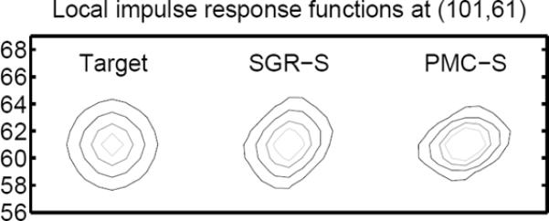
Contours of LIRs: Target, SGR-S (single gate), PMC-S (four gates with motion). Incorporated motion information may introduce additional non-uniform and anisotropic spatial resolution to the static case.

There have been many studies of the spatial resolution properties of static image reconstruction [21]–[27] and dynamic image reconstruction [28]. Regularizers that provide nearly uniform spatial resolution, or “certainty-based” regularizers, have been proposed for quadratic regularization with PET [21], fully 3D PET [23], and for nonquadratic regularizers with PET [26]. Regularizers that achieve approximately uniform and isotropic spatial resolution have been developed for PET [24], [25] and 2D fan-beam CT [27]. However, there has been little such research for regularized MCIR methods.

This paper investigates the spatial resolution properties of three popular MCIR methods (PMC, PMM, and MTR). Based on this analysis, we propose quadratic regularizers that can achieve approximately isotropic and uniform spatial resolution even in the presence of nonrigid motion and for heteroscedastic log-likelihoods. For regularizer design, we extend the “analytical approach” [27], [29] to MCIR methods [30] for the case of known nonrigid motion. The known motion assumption can be suitable for some multi-modal medical imaging applications such as PET-CT [9], [10], [12] and PET-MR systems [16].

This paper is organized as follows. Section II presents measurement and motion/warp models for MCIR methods. Section III introduces three different MCIR methods and their LIRs. Section IV investigates how to design spatial regularizers for MCIR methods that provide approximately uniform and isotropic spatial resolution for nonrigid motion by extending analytical approach. Section V illustrates the proposed spatial regularizers by 2D PET simulations with nonrigid motion.

II. MCIR MODELS

A. Measurement model

Most medical imaging systems cannot capture an entire dataset instantaneously, but rather record a sequence of measurements over some time interval. For example, X-ray CT scanners acquire about 1000 projection views during a sub-second rotation around the object. MCIR methods are needed when the time-varying object $f(\overrightarrow{x},t)$ has non-negligible motion during such an acquisition interval. Often one can use gating or temporal binning to group the measurements into M sets, called “frames” here, such that object motion is negligible within each frame, and then one can focus on the object motion between frames. This type of discrete approximation to continuous object motion is ubiquitous in MCIR models and we adopt it here as well. Let y_m denote the vector of measurements associated with the mth frame, e.g., a frame in a gated scan. We assume the time varying object $f(\overrightarrow{x},t)$ is approximately motionless during the acquisition of each y_m. Let t_m denote the time associated with the mth frame, and let ${\mathit{f}}_m=(f({\overrightarrow{x}}_1,t_m),\dots ,f({\overrightarrow{x}}_N,t_m))$ denote a spatial discretization of the object f(., t_m) where ${\overrightarrow{x}}_j$ denotes the center of the jth voxel for j = 1, …, N, and N denotes the number of voxels. We assume that the measurements are related to the object linearly as follows:

$${\mathit{y}}_m={\mathit{A}}_m{\mathit{f}}_m+{∊}_m,m=1,\dots ,M,$$ (1)

where A_m denotes the system model for the mth frame, ∊_m denotes noise, and M is the number of gates or frames. We allow the system model A_m to possibly differ for each frame to accommodate systems that rotate such as gated SPECT or CT or that can otherwise change sampling properties dynamically such as MRI. In some cases, we assume that A_m = D_mA₀, ∀m where D_m is a diagonal matrix (e.g., PET scan, gated MRI scan with fixed k-space sampling, or a video sequence).

B. Basic warp model

For a given spatial transformation $T_{m,n}:{\mathbb{R}}^d\to {\mathbb{R}}^d$, we can define a warp operator τ_m,n as follows:

$$f(\overrightarrow{x},t_m)=\left({\mathcal{T}}_{m,n}f\right)(\overrightarrow{x},t_n)\triangleq f(T_{m,n}\left(\overrightarrow{x}\right),t_n),$$ (2)

where $\overrightarrow{x}$ belongs to an image domain ${\mathbb{R}}^d$ at time t_m and d is usually 2 or 3. We can discretize the warp τ_m,n to define a map from the image f_n to the image f_m as follows:

$${\mathit{f}}_m={\mathit{T}}_{m,n}{\mathit{f}}_n,n,m=1,\dots ,M.$$ (3)

For applications with periodic motion, we can additionally define ${\mathit{f}}_{M+1}\triangleq {\mathit{f}}_1$ and ${\mathit{T}}_{M+1,M}\triangleq {\mathit{T}}_{1,M}$. The N × N matrix T_m,n can be implemented with any interpolation method; we used a B-spline based image warp [31] for our empirical results. Let $\mid \nabla T_{m,n}\left(\overrightarrow{x}\right)\mid$ denote the determinant of the Jacobian matrix of a transform $T_{m,n}\left(\overrightarrow{x}\right)$ for a warp T_m,n. Throughout we assume the warps T_m,n (or equivalently T_m,n or T_m,n) are known.

C. Total activity-preserving warp model

In many medical imaging applications, total activity (or total mass) is preserved during the scan [32], [33] and this property has been used in some MCIR methods [34]. To enforce this constraint, the operator τ_m,n must not change the total activity of an image. To preserve total activity (or mass), one can define a modification of the operator τ_m,n that uses the Jacobian determinant of T_m,n:

$$\begin{array}{cc}\hfill f(\overrightarrow{x},t_m)& =\left({\mathring{\mathcal{T}}}_{m,n}f\right)(\overrightarrow{x},t_n)\hfill \\ \hfill & \triangleq {\mid \nabla T_{m,n}\left(\overrightarrow{x}\right)\mid }^{p}f(T_{m,n}\left(\overrightarrow{x}\right),t_n)\hfill \end{array}$$ (4)

where p = 1. To verify that total activity is preserved, note that

$$\begin{array}{cc}\hfill {\int }_{{\mathbb{R}}^d}f(\overrightarrow{x},t_m)d\overrightarrow{x}& ={\int }_{{\mathbb{R}}^d}\mid \nabla T_{m,n}\left(\overrightarrow{x}\right)\mid f(T_{m,n}\left(\overrightarrow{x}\right),t_n)d\overrightarrow{x}\hfill \\ \hfill & ={\int }_{{\mathbb{R}}^d}f(\overrightarrow{y},t_n)d\overrightarrow{y}\hfill \end{array}$$ (5)

where $\overrightarrow{y}=T_{m,n}\left(\overrightarrow{x}\right)$. Similarly, we can define a discrete-space warp corresponding to (4) that approximately preserves total activity:

$${\mathit{f}}_m={\mathring{\mathit{T}}}_{m,n}{\mathit{f}}_n,n,m=1,\dots ,M,$$ (6)

where

$${\mathring{\mathit{T}}}_{m,n}\triangleq \mathit{D}\left({\mid \nabla T_{m,n}\left({\overrightarrow{x}}_j\right)\mid }^p\right){\mathit{T}}_{m,n}$$ (7)

and $\mathit{D}\left({\mid \nabla T_{m,n}\left({\overrightarrow{x}}_j\right)\mid }^p\right)$ is a N × N diagonal matrix with elements $\left\{{\mid \nabla T_{m,n}\left({\overrightarrow{x}}_j\right)\mid }^p\right\}$, j = 1, …, N and p = 1. We use (4) and (6) for the analyses in this paper, but one can simply let p = 0 if a total activity-preserving model is not needed.

The warp operator τ_m,n in (2) acts pointwise, so its discretized version in (3) also acts approximately pointwise. Therefore, the diagonal matrix in (7) that is applied to the left hand side of T_m,n can be replaced (approximately) by a closely related diagonal matrix on the right hand side of T_m,n by simply adjusting the spatial coordinates as follows:

$$\begin{array}{cc}\hfill \mathit{D}\left({\mid \nabla T_{m,n}\left({\overrightarrow{x}}_j\right)\mid }^p\right){\mathit{T}}_{m,n}& \approx {\mathit{T}}_{m,n}\mathit{D}\left({\mid \nabla T_{m,n}\left(T_{n,m}\left({\overrightarrow{x}}_j\right)\right)\mid }^p\right)\hfill \\ \hfill & \approx {\mathit{T}}_{m,n}\mathit{D}\left({\mid \nabla T_{m,n}\left({\overrightarrow{x}}_j\right)\mid }^{-p}\right)\hfill \end{array}$$ (8)

where $\mid \nabla T_{m,n}\left(T_{n,m}\left({\overrightarrow{x}}_j\right)\right)\mid \mid \nabla T_{n,m}\left({\overrightarrow{x}}_j\right)\mid =1$ by the chain rule.

In some cases, we assume that invertibility, symmetry, and transitivity properties hold for T̊_m,n,, i.e.,

$$\mid \nabla T_{m,n}\mid >0,\forall n,m,$$ (9)

$${\mathring{\mathit{T}}}_{m,n}^{-1}={\mathring{\mathit{T}}}_{n,m},\forall n,m,$$ (10)

$${\mathring{\mathit{T}}}_{m,n}={\mathring{\mathit{T}}}_{m,m-1}\dots {\mathring{\mathit{T}}}_{n+1,n},\forall m>n.$$ (11)

These assumptions are reasonable for usual patient motion such as respiratory or cardiac motion. In practice, one can estimate motion models that satisfy these conditions [35], [36].

III. Local Impulse Response for Mcir

We consider three MCIR methods: PMC [3]–[5], PMM [8]–[14], [17], [19], and MTR [6], [7], [20], [37]. Here we treat the nonrigid motion information as predetermined (known). In this section, we derive the LIRs for regularized versions of these MCIR methods.

A. Single gated reconstruction (SGR)

Often one can reconstruct each image ${\widehat{\mathit{f}}}_m$ from the corresponding measurement y_m based on the model (1) and some prior knowledge (e.g., a smoothness prior). A single gated (frame) reconstruction (SGR) can be obtained as follows:

$${\widehat{\mathit{f}}}_m\triangleq \underset{{\mathit{f}}_m}{\text{argmin}}\mathrm{L}({\mathit{y}}_m,{\mathit{A}}_m{\mathit{f}}_m)+\eta \mathrm{R}\left({\mathit{f}}_m\right)$$ (12)

where L is a likelihood function derived from (1), R is a spatial regularizer, and η is a spatial regularization parameter.

For any single-frame estimator ${\widehat{\mathit{f}}}_m\left({\mathit{y}}_m\right)$, one can define the LIR for the jth pixel as

$${\mathit{l}}_m^j\triangleq \underset{\delta \to 0}{\text{lim}}\frac{{\widehat{\mathit{f}}}_m\left({\stackrel{‒}{\mathit{y}}}_m({\mathit{f}}_m+\delta e_j)\right)-{\widehat{\mathit{f}}}_m\left({\stackrel{‒}{\mathit{y}}}_m\left({\mathit{f}}_m\right)\right)}{\delta }$$ (13)

where ${\stackrel{‒}{y}}_m$ is the mean of y_m and e_j is a unit vector with one at the jth element. If L in (12) is a negative Poisson log-likelihood function (i.e., L(y, u) ≜ Σ_i[u]_i−[y]_i log[u_i]), then one can show that the LIR in (13) can be approximated [21]:

$$\begin{array}{cc}\hfill {\mathit{l}}_m^j& \approx {[{\mathit{A}}_m^{\prime }{\mathit{W}}_m{\mathit{A}}_m+\eta {\mathit{R}}_m]}^{-1}{\mathit{A}}_m^{\prime }{\mathit{W}}_m{\mathit{A}}_m{\mathit{e}}_j\hfill \\ \hfill & \approx {[{\mathit{F}}_m+\eta {\mathit{R}}_m]}^{-1}{\mathit{F}}_m{\mathit{e}}_j\hfill \end{array}$$ (14)

where ${\mathit{W}}_m\triangleq \mathit{D}(1∕{\left[{\stackrel{‒}{\mathit{y}}}_m\left({\mathit{f}}_m\right)\right]}_i)$ is a diagonal matrix, the Hessian of the regularizer is ${\mathit{R}}_m\triangleq {\nabla }^2\text{R}\left({\check{\mathit{f}}}_m\right)$, ${\check{\mathit{f}}}_m={\widehat{\mathit{f}}}_m\left({\stackrel{‒}{y}}_m\left({\mathit{f}}_m\right)\right)$, “′” denotes matrix transpose, and the Fisher information matrix is

$${\mathit{F}}_m\triangleq {\mathit{A}}_m^{\prime }{\mathit{W}}_m{\mathit{A}}_m.$$

Equation (14) implies that the LIR of (1) for a Poisson likelihood can be approximated with the LIR of (1) for a penalized weighted least square (PWLS) likelihood. Thus, the analysis in the paper also applies to any PWLS model. Sometimes, a regularizer depends on the noiseless projection ${\stackrel{‒}{\mathit{y}}}_m\left({\mathit{f}}_m\right)$, which is unavailable. However, as shown in [21], a plug-in approach that replaces ${\stackrel{‒}{\mathit{y}}}_m\left({\mathit{f}}_m\right)$ by y_m (or smoothed y_m) works well for the regularization design since A_m contains blurring operator. In the simulation, we will show that this is also the case for MCIRs.

B. Post-reconstruction motion correction (PMC)

Once the frames ${\widehat{f}}_1,\dots ,{\widehat{f}}_M$ are reconstructed individually from (12) for all m, one way to improve the SNR would be to average all of them. However, the resulting image would be contaminated by motion blur due to the mismatch between frames. Using the motion information to map each image f_m to a single image's coordinates can reduce motion artifacts. Without loss of generality, we chose f₁ as our reference image. Using (6) and (12), a natural definition for the PMC estimator is the following motion-compensated average:

$${\widehat{\mathit{f}}}_{\text{PMC}}\triangleq \frac{1}{M}\sum _{m=1}^M{\mathring{\mathit{T}}}_{1,m}{\widehat{\mathit{f}}}_m.$$ (15)

Using (14), (10), and (6), one can derive the LIR for the PMC estimator (15) at the jth pixel of the first frame as follows:

$$\begin{array}{cc}\hfill {\mathit{l}}_{\text{PMC}}^j& \approx \frac{1}{M}\sum _{m=1}^M{\mathring{\mathit{T}}}_{1,m}{[{\mathit{F}}_m+\eta {\mathit{R}}_m]}^{-1}{\mathit{F}}_m{\mathring{\mathit{T}}}_{m,1}{\mathit{e}}_j\hfill \\ \hfill & \approx \frac{1}{M}\sum _{m=1}^M{[{\mathring{\mathit{F}}}_m+\eta {\mathring{\mathit{R}}}_m]}^{-1}{\mathring{\mathit{F}}}_m{\mathit{e}}_j\hfill \end{array}$$ (16)

where ${\mathring{\mathit{F}}}_m\triangleq {\mathring{\mathit{T}}}_{m,1}^{\prime }{\mathit{F}}_m{\mathring{\mathit{T}}}_{m,1}$ and ${\mathring{\mathit{R}}}_m\triangleq {\mathring{\mathit{T}}}_{m,1}^{\prime }{\mathit{R}}_m{\mathring{\mathit{T}}}_{m,1}$. We used ${\mathring{\mathit{T}}}_{m,1}{\mathit{e}}_j$ instead of e_j as an impulse for the mth frame, which corresponds to an impulse in the first frame.

C. Parametric motion model (PMM)

To derive the LIR of the PMM approach, we first must choose a reference image frame among {f₁, …, f_M}. With-out loss of generality, we assume that f₁ is our reference image frame. Then, combining the measurement model (1) with the warp (6) yields a new measurement model that depends only on the image f₁ instead of the all images f_m:

$${\mathit{y}}_m={\mathit{A}}_m{\mathring{\mathit{T}}}_{m,1}{\mathit{f}}_1+{∊}_m,m=1,\dots ,M.$$

Stacking up these models yields the overall model

$${\mathit{y}}_{\mathrm{c}}={\mathit{A}}_{\mathrm{d}}{\mathring{T}}_{\mathrm{c}}{\mathit{f}}_1+{∊}_{\mathrm{c}},$$ (17)

where the components are each stacked accordingly:

$$\begin{array}{cc}\hfill & {\mathit{y}}_{\mathrm{c}}\triangleq {[{\mathit{y}}_1^{\prime },\dots ,{\mathit{y}}_M^{\prime }]}^{\prime },\hfill \\ \hfill & {\mathit{A}}_{\mathrm{d}}\triangleq \text{diag}\{{\mathit{A}}_1,\dots ,{\mathit{A}}_M\},\hfill \\ \hfill & {\mathring{\mathit{T}}}_{\mathrm{c}}\triangleq {[\mathit{I},{\mathring{\mathit{T}}}_{2,1}^{\prime },\dots ,{\mathring{\mathit{T}}}_{M,1}^{\prime }]}^{\prime },\hfill \\ \hfill & {∊}_{\mathrm{c}}\triangleq {[{∊}_1^{\prime },\dots ,{∊}_M^{\prime }]}^{\prime }.\hfill \end{array}$$ (18)

The PMM estimator for the measurement model (17) with a spatial regularizer is

$${\widehat{\mathit{f}}}_{\text{PMM}}\triangleq \underset{{\mathit{f}}_1}{\text{argmin}}\mathrm{L}({\mathit{y}}_{\mathrm{c}},{\mathit{A}}_{\mathrm{d}}{\mathring{\mathit{T}}}_{\mathrm{c}}{\mathit{f}}_1)+\eta \mathrm{R}\left({\mathit{f}}_1\right)$$ (19)

where L is a negative likelihood function and R is a spatial regularizer.

For the linear measurement model (17) with a negative Poisson log-likelihood function L, similar to (14) one can approximate the LIR (as defined in (13)) for the PMM estimator (19) at the jth pixel as follows:

$${\mathit{l}}_{\text{PMM}}^j\approx {[{\mathring{\mathit{T}}}_{\mathrm{c}}^{\prime }{\mathit{F}}_{\mathrm{d}}{\mathring{\mathit{T}}}_{\mathrm{c}}+\eta {\mathit{R}}_{\text{PMM}}]}^{-1}{\mathring{\mathit{T}}}_{\mathrm{c}}^{\prime }{\mathit{F}}_{\mathrm{d}}{\mathring{\mathit{T}}}_{\mathrm{c}}{\mathit{e}}_j$$ (20)

where ${\mathit{F}}_{\text{d}}\triangleq {\mathit{A}}_{\text{d}}^{\prime }{\mathit{W}}_{\text{d}}{\mathit{A}}_{\text{d}}=\text{diag}\{{\mathit{F}}_1,\dots ,{\mathit{F}}_M\}$ is a block-diagonal matrix, ${\mathit{W}}_{\text{d}}\triangleq \mathit{D}(1∕{\left[{\stackrel{‒}{y}}_{\text{c}}\left({\mathit{f}}_1\right)\right]}_i)$ is a diagonal matrix, ${\stackrel{‒}{y}}_c$ is the mean of y_c, ${\mathit{R}}_{\text{PMM}}\triangleq {\nabla }^2\text{R}\left({\check{\mathit{f}}}_{\text{PMM}}\right)$, and ${\check{\mathit{f}}}_{\text{PMM}}={\widehat{\mathit{f}}}_{\text{PMM}}\left({\stackrel{‒}{y}}_c\left({\mathit{f}}_1\right)\right)$. Note that

$${\mathring{\mathit{T}}}_{\mathrm{c}}^{\prime }{\mathit{F}}_{\mathrm{d}}{\mathring{\mathit{T}}}_{\mathrm{c}}=\sum _{m=1}^M{\mathring{\mathit{T}}}_{m,1}^{\prime }{\mathit{F}}_m{\mathring{\mathit{T}}}_{m,1}=\sum _{m=1}^M{\mathring{\mathit{F}}}_m.$$ (21)

Using (20) and (21), we can rewrite the LIR of the PMM estimator at the jth pixel as

$${\mathit{l}}_{\text{PMM}}^j\approx {\left[\sum _{m=1}^M{\mathring{\mathit{F}}}_m+\eta {\mathit{R}}_{\text{PMM}}\right]}^{-1}\sum _{m=1}^M{\mathring{\mathit{F}}}_m{\mathit{e}}_j.$$ (22)

D. Motion-compensated temporal regularization (MTR)

The MTR method incorporates the motion information that matches two adjacent images into a temporal regularization term [6], [7]:

$${\Vert {\mathit{f}}_{m+1}-{\mathring{\mathit{T}}}_{m+1,m}{\mathit{f}}_m\Vert }_2^2.$$ (23)

for m = 1, …, M − 1. This penalty is added to the cost function in (12) for all m to define the MTR cost function.

Equations (12) for all m and (23) can be represented in a simpler vector-matrix notation. First, stack up (1) for all m as follows:

$${\mathit{y}}_{\mathrm{c}}={\mathit{A}}_{\mathrm{d}}{\mathit{f}}_{\mathrm{c}}+{∊}_{\mathrm{c}},$$ (24)

where ${\mathit{f}}_{\text{c}}=[{\mathit{f}}_1^{\prime },\cdots ,{\mathit{f}}_M^{\prime }]\prime$ and A_d, ∊_c were defined in (18). Then, the MTR estimator based on (23), (24), and a spatial regularizer is where L is

$${\widehat{\mathit{f}}}_{\text{MTR}}\triangleq \underset{{\mathit{f}}_{\mathrm{c}}}{\text{argmin}}\mathrm{L}({\mathit{y}}_{\mathrm{c}},{\mathit{A}}_{\mathrm{d}}{\mathit{f}}_{\mathrm{c}})+\eta \mathrm{R}\left({\mathit{f}}_{\mathrm{c}}\right)+\zeta {\Vert {\mathit{T}}_{\text{time}}{\mathit{f}}_{\mathrm{c}}\Vert }_2^2$$ (25)

where L is a negative likelihood function from the noise model of (24), R is a spatial regularizer, ζ is a temporal regularization parameter, and the temporal differencing matrix is

$${\mathit{T}}_{\text{time}}\triangleq \left[\begin{array}{cccc}\hfill -{\mathring{\mathit{T}}}_{2,1}\hfill & \hfill \mathit{I}\hfill & \hfill \hfill & \hfill \hfill \\ \hfill \hfill & \hfill \ddots \hfill & \hfill \ddots \hfill & \hfill \hfill \\ \hfill \hfill & \hfill \hfill & \hfill -{\mathring{\mathit{T}}}_{M,M-1}\hfill & \hfill \mathit{I}\hfill \end{array}\right].$$ (26)

We may also modify T_time for periodic (or pseudo-periodic) image sequences by adding a row corresponding to the term ${\Vert {\mathit{f}}_1-{\mathring{\mathit{T}}}_{1,M}{\mathit{f}}_M\Vert }^2$. Note that unlike the PMM method that estimates one frame, MTR estimates all image frames.

For the MTR estimator (25) with a negative Poisson log-likelihood function L, one can derive the LIR of the MTR estimator at the jth pixel as follows:

$${\mathit{l}}_{\text{MTR}}^j\approx {[{\mathit{F}}_{\mathrm{d}}+\eta {\mathit{R}}_{\mathrm{d}}+\zeta {\mathit{R}}_{\text{time}}]}^{-1}{\mathit{F}}_{\mathrm{d}}{\mathit{e}}_{\mathrm{c}}^j$$ (27)

where R_d ≜ diag {R₁, …, R_M}, ${\mathit{R}}_{\text{time}}\triangleq {\mathit{T}}_{\text{time}}^{\prime }{\mathit{T}}_{\text{time}}$, and we define an impulse vector for all frames at jth voxel of the first frame as

$${\mathit{e}}_{\mathrm{c}}^j\triangleq [{\mathit{e}}_j^{\prime },\left({\mathring{\mathit{T}}}_{2,1}{\mathit{e}}_j\right)\prime ,\cdots ,\left({\mathring{\mathit{T}}}_{M,1}{\mathit{e}}_j\right)\prime ]\prime$$ (28)

which is the same as the impulse for the PMC in (16). We can interpret the LIR of MTR (27) as follows. For ζ = 0, the LIR of MTR at the jth pixel would be the same as the LIRs of SGR (14) for all m. For $\zeta >0,\zeta {\Vert {\mathit{T}}_{\text{time}}{\mathit{f}}_{\text{c}}\Vert }_2^2$ term in (25) encourages each LIR of the mth frame to be the same as one another, which can result in different spatial resolution for different ζ.

E. Local impulse response (LIR) summary

The main results of this section are the LIR expressions (16), (22), and (27) for the PMC, PMM, and MTR methods for MCIR respectively. Readers familiar with [21] will recognize that these LIR expressions reflect non-uniform and anisotropic spatial resolution, both due to heteroscedastic noise and due to nonrigid motion for standard regularizers. The next section presents regularization design methods that can provide approximately uniform and isotropic spatial resolution.

IV. Spatial regularizer designs for MCIR

In this section, we present ways to design spatial regularizers of MCIR methods to provide approximately uniform and isotropic spatial resolution that does not depend on object-specific measurement statistics and given object-specific non-rigid motion. We extend the so-called analytical approach for regularizer design [29] to MCIR cases.

For the analysis in this section, we focus on 2D PET. We consider an ideal tomography system, i.e., we ignore detector blur; nevertheless we conjecture that the regularization designs are also useful in the presence of detector blur. We assume that

$${\mathit{A}}_m={\mathit{D}}_m{\mathit{A}}_0,m=1,\cdots ,M,$$ (29)

where D_m denotes a diagonal matrix for patient-dependent attenuation and detector efficiency for the mth frame, and A₀ is a system geometry. We assume known and well-aligned attenuation map (i.e., D_m is given), which can be the case for PET-CT [38] or PET-MR [39]. We still allow the warp T_m,1 to differ for each m.

For nonrigid motion, we assume that given nonrigid motion is locally affine [40]. This can be viewed as a first order Taylor expansion of general nonrigid motion, which can be a good approximation locally for smooth motion. We limit our analysis to 2D cases and focus on using a first-order difference matrix as a spatial regularizer.

A. Single gated reconstruction (SGR)

We first briefly review the “conventional” analytical approach for designing a regularizer that provides approximately uniform and isotropic spatial resolution for static image reconstruction [27], [29]. This SGR method is also suitable when reconstructing an individual frame, e.g., f_m, from the corresponding measurement y_m. However, the empirical results in Section V show that this conventional regularizer does not provide the intended spatial resolution for any of the MCIR methods described above, so we provide new regularization designs for MCIR methods in subsequent subsections.

We focus on quadratic regularization methods using first-order finite differences as follows:

$${\mathit{f}}_m^{\prime }{\mathit{R}}_m{\mathit{f}}_m={\Vert {\mathit{C}}_m{\mathit{f}}_m\Vert }^2\triangleq \sum _j\sum _{l=1}^L{r}_{l,m}^j{\left((c_l\ast \ast f_m)\left[{\overrightarrow{n}}_j\right]\right)}^2,$$ (30)

where ** denotes 2D convolution, f_m[${\overrightarrow{n}}_j$] denotes the 2D array corresponding to the lexicographically ordered vector f_m, j is the lexicographic index of the pixel at ${\overrightarrow{n}}_j$ and

$$c_l\left[{\overrightarrow{n}}_j\right]=\frac{1}{{\Vert {\overrightarrow{m}}_l\Vert }_2}({\delta }_2\left[{\overrightarrow{n}}_j\right]-{\delta }_2[{\overrightarrow{n}}_j-{\overrightarrow{m}}_l]),$$ (31)

where {${\overrightarrow{m}}_l$} denote the spatial offsets of the jth pixel's neighbors and δ₂[${\overrightarrow{n}}_j$] denotes the 2D Kronecker impulse. For our empirical results, we used the usual 8-pixel 2D neighborhood with $\left\{{\overrightarrow{m}}_l\right\}=\{(1,0),(0,1),(1,1),(1,-1)\}$.

For the single-frame estimator ${\widehat{\mathit{f}}}_m\left({\mathit{y}}_m\right)$ in (12) with (29), one can rewrite the LIR (14) for SGR as

$${\mathit{l}}_m^j\approx {[{\mathit{F}}_m+\eta {\mathit{R}}_m]}^{-1}{\mathit{F}}_m{\mathit{e}}_j$$ (32)

where ${\mathit{F}}_m\triangleq {\mathit{A}}_0^{\prime }{\tilde{\mathit{W}}}_m{\mathit{A}}_0$ and ${\tilde{\mathit{W}}}_m\triangleq {\mathit{D}}_m^{\prime }{\mathit{W}}_m{\mathit{D}}_m$ is a diagonal matrix. We would like to design the regularizer R_m (i.e., to select {$r_{l,m}^j$} in (30)) so that the LIR closely matches some target point spread function (PSF). A reasonable target for the jth pixel is

$${\mathit{l}}_0^j={[{\mathit{A}}_0^{\prime }{\mathit{A}}_0+\eta {\mathit{R}}_0]}^{-1}{\mathit{A}}_0^{\prime }{\mathit{A}}_0{\mathit{e}}_j$$ (33)

which is the (often shift-invariant) LIR of a penalized un-weighted least square (PULS) estimator, and R₀ denotes the Hessian of a standard shift-invariant quadratic regularizer. If we assume slowly varying weights in ${\tilde{\mathit{W}}}_m$ at the jth pixel, then ${\mathit{A}}_0^{\prime }{\tilde{\mathit{W}}}_m{\mathit{A}}_0$ becomes approximately a locally circulant matrix. One can show that “${\mathit{l}}_m^j\approx {\mathit{l}}_0^j$” approximately reduces to

$${\mathit{R}}_0{\mathit{A}}_0^{\prime }{\tilde{\mathit{W}}}_m{\mathit{A}}_0{\mathit{e}}_j\approx {\mathit{R}}_m{\mathit{A}}_0^{\prime }{\mathit{A}}_0{\mathit{e}}_j.$$ (34)

Therefore, our regularization design becomes an optimization problem with respect to R_m (or {$r_{l,m}^j$}) for all j and m:

$$\underset{{\left\{r_{l,m}^j\right\}}_{l=1}^L\ge 0}{\text{argmin}}{\Vert {\mathit{R}}_0{\mathit{A}}_0^{\prime }{\tilde{\mathit{W}}}_m{\mathit{A}}_0{\mathit{e}}_j-{\mathit{R}}_m{\mathit{A}}_0^{\prime }{\mathit{A}}_0{\mathit{e}}_j\Vert }_2^2$$ (35)

where R_m is the function of {$r_{l,m}^j$} for all l and j as given in (30).

An analytical formulation can simplify (35) by using a frequency domain representation. For polar coordinates (ρ, φ) in frequency space, we write ${\mathit{A}}_0^{\prime }{\mathit{A}}_0\equiv {\mid B\left(\rho \right)\mid }^2∕\rho$ to indicate that ${\mathit{A}}_0^{\prime }{\mathit{A}}_0$ is a locally shift-invariant operator with local frequency response |B(ρ)|² /ρ where B(·) denotes the frequency response of a typical radial blur function b(r) (e.g., the blur at the center of a single projection view). For a standard quadratic penalty function R₀ (i.e. ∫∥▽f_m∥²), one can show that R₀ ≡ (2πρ)², and the quadratic function (30) becomes ${\mathit{R}}_m\equiv {\Sigma }_{l=1}^L{r}_{l,m}^j{\left(2\pi \rho \right)}^2{\text{cos}}^2(\phi -{\phi }_l)$, where ${\phi }_l=\angle {\overrightarrow{m}}_l$. One can also show by using the Fourier slice theorem and assuming the local shift invariance of ${\mathit{A}}_0^{\prime }{\tilde{\mathit{W}}}_m{\mathit{A}}_0$ (slowly varying ${\tilde{\mathit{W}}}_m$) that [41]

$${\mathit{F}}_m={\mathit{A}}_0^{\prime }{\tilde{\mathit{W}}}_m{\mathit{A}}_0\equiv \frac{{\stackrel{‒}{w}}_m(\phi ;{\overrightarrow{x}}_j){\mid B_{\phi }^j\left(\rho \right)\mid }^2}{\rho },$$ (36)

where $B_{\phi }^j(\cdot )$ denotes the (local) frequency response of the detector response $b_{\phi }^j\left(r\right)$ at angle φ local to where the jth pixel projects onto the detector at that angle, and the angular-dependent weighting ${\stackrel{‒}{w}}_m(\phi ;{\overrightarrow{x}}_j)$ for the jth pixel is

(37)

where ${\mathcal{I}}_{\phi }$ is the set of rays at the angle φ, a_ij, ≜ [A₀]_ij, and ${\tilde{w}}_{m,i}\triangleq {\left[{\tilde{\mathit{W}}}_m\right]}_{ii}$. We simplify (35) to the following cost function with respect to {$r_{l,m}^j$} for each m and j

$$\underset{{\left\{r_{l,m}^j\right\}}_{l=1}^L\ge 0}{\text{argmin}}\Psi \left(r_{l,m}^j,{\stackrel{‒}{w}}_m(\phi ;{\overrightarrow{x}}_j)\right)$$ (38)

where

$$\Psi \left(r_{l,m}^j,w\right)\triangleq {\int }_0^{\pi }{\left[w-\sum _{l=1}^L{r}_{l,m}^j{\text{cos}}^2(\phi -{\phi }_l)\right]}^2\mathrm{d}\phi .$$ (39)

We can solve (38) analytically using Karush-Kuhn-Tucker conditions or iteratively using an iterative non-negative least squares method. This summarizes [27], [29] for static 2D imaging. We extend these methods to MCIR next.

B. Post-reconstruction motion correction (PMC)

We would like to design regularizers R_m that can approximate ${\mathit{l}}_{\text{PMC}}^j\approx {\mathit{l}}_0^j$ for all j. Equations (16) and (33) show that if we design a regularizer R_m such that

$${[{\mathring{\mathit{F}}}_m+\eta {\mathring{\mathit{R}}}_m]}^{-1}{\mathring{\mathit{F}}}_m{\mathit{e}}_j\approx {[{\mathit{F}}_0+\eta {\mathit{R}}_0]}^{-1}{\mathit{F}}_0{\mathit{e}}_j$$ (40)

for all m where ${\mathit{F}}_0\triangleq {\mathit{A}}_0^{\prime }{\mathit{A}}_0$, then, we can achieve ${\mathit{l}}_{\text{PMC}}^j\approx {\mathit{l}}_0^j$. Equivalently, we want to design R_m (or $r_{l,m}^j$) such that

$${[{\mathit{F}}_m+\eta {\mathit{R}}_m]}^{-1}{\mathit{F}}_m{\mathit{e}}_j\approx {\mathring{\mathit{T}}}_{m,1}{[{\mathit{F}}_0+\eta {\mathit{R}}_0]}^{-1}{\mathit{F}}_0{\mathring{\mathit{T}}}_{1,m}{\mathit{e}}_j$$ (41)

for all m. For small η, [F₀+ηR₀]⁻¹F₀ will be approximately diagonal, so by (7) and (8), we can cancel the diagonal matrices in ${\mathring{\mathit{T}}}_{m,1}$ and ${\mathring{\mathit{T}}}_{1,m}$ so that (41) becomes

$${[{\mathit{F}}_m+\eta {\mathit{R}}_m]}^{-1}{\mathit{F}}_m{\mathit{e}}_j\approx {\mathit{T}}_{m,1}{[{\mathit{F}}_0+\eta {\mathit{R}}_0]}^{-1}{\mathit{F}}_0{\mathit{T}}_{1,m}{\mathit{e}}_j.$$ (42)

By assuming the warp is locally affine and ${\mathring{\mathit{T}}}_{m,1}{\mathit{F}}_0{\mathring{\mathit{T}}}_{1,m}$ is approximately circulant locally, (42) becomes the following optimization problem for each m and j:

$$\underset{{\left\{r_{l,m}^j\right\}}_{l=1}^L\ge 0}{\text{argmin}}{\Vert {\mathit{T}}_{m,1}{\mathit{R}}_0{\mathit{T}}_{1,m}{\mathit{F}}_m{\mathit{e}}_j-{\mathit{R}}_m{\mathit{T}}_{m,1}{\mathit{F}}_0{\mathit{T}}_{1,m}{\mathit{e}}_j\Vert }_2.$$ (43)

We need to determine an analytical form for T_m,1R₀T_1,m and T_m,1F₀T_1,m to solve (43) efficiently. With the results of Appendices A and B (assuming locally affine transforms T_m,1 and T_1,m), one can show the equivalent continuous forms of T_m,1F₀T_1,m and T_m,1R₀T_1,m at the jth pixel are as follows:

$${\mathit{T}}_{m,1}{\mathit{F}}_0{\mathit{T}}_{1,m}\equiv \frac{{\mid B\left(\rho \right)\mid }^2}{\rho {\Vert \nabla T_{1,m}\left({\overrightarrow{x}}_j\right)\prime (\text{cos}\phi ,\text{sin}\phi )\prime \Vert }_2}$$ (44)

$${\mathit{T}}_{m,1}{\mathit{R}}_0{\mathit{T}}_{1,m}\equiv {\left(2\pi \rho \right)}^2{\Vert \nabla T_{1,m}\left({\overrightarrow{x}}_j\right)\prime (\text{cos}\phi ,\text{sin}\phi )\prime \Vert }_2^2$$ (45)

where we ignore detector blur (i.e., b(r) ≈ δ(r) or B(ρ) ≈ 1) in (45). Thus, using a procedure similar to Section IV-A, we perform (43) by minimizing the following cost function with respect to $\left\{r_{l,m}^j\right\}$ for each m and j:

$$\underset{{\left\{r_{l,m}^j\right\}}_{l=1}^L\ge 0}{\text{argmin}}\Psi \left(r_{l,m}^j,\stackrel{‒}{w}\text{PMC},m(\phi ;{\overrightarrow{x}}_j)\right)$$ (46)

where the angular-dependent weighting for the jth pixel is

and ${\stackrel{‒}{w}}_m(\phi ;{\overrightarrow{x}}_j)$ is defined in (37). ${\stackrel{‒}{w}}_m(\phi ;{\overrightarrow{x}}_j)$ describes the non-uniformity and anisotropy of the spatial resolution due to the interaction between the likelihood and the regularizer, which is also observed in (38) for SGR. ${\Vert \nabla T_{1,m}\left({\overrightarrow{x}}_j\right)\prime (\text{cos}\phi ,\text{sin}\phi )\prime \Vert }_2^3$ is an additional term to explain the non-uniformity and anisotropy due to motion. As mentioned in Section IV-A, one can solve optimization problems of the form (46) analytically or iteratively [27], [29].

C. Parametric motion model (PMM)

For uniform and isotropic spatial resolution, we would like to design R_PMM (which is of the form (30) with $r_l^j$) to satisfy ${\mathit{l}}_{\text{PMM}}^j\approx {\mathit{l}}_0^j$ from (22) and (33). By assuming a locally affine transform, ${\mathring{\mathit{F}}}_m$ in (22) will be a locally circulant matrix at the jth voxel, which reduces ${\mathit{l}}_{\text{PMM}}^j\approx {\mathit{l}}_0^j$ to the following simpler optimization problem:

$$\underset{{\left\{r_l^j\right\}}_{l=1}^L\ge 0}{\text{argmin}}{\Vert {\mathit{R}}_0\sum _{m=1}^M{\mathring{\mathit{F}}}_m{\mathit{e}}_j-{\mathit{R}}_{\text{PMM}}{\mathit{F}}_0{\mathit{e}}_j\Vert }_2$$ (47)

for all j. Ignoring detector blur, one can use Appendix B to show that the analytical form for ${\mathring{\mathit{F}}}_m$ is

$${\mathring{\mathit{F}}}_m\equiv \frac{{\stackrel{‒}{w}}_m(\tilde{\phi };T_{m,1}^{-1}\left({\overrightarrow{x}}_j\right)){\mid \nabla T_{m,1}\left({\overrightarrow{x}}_j\right)\prime \mid }^{2p-1}}{\rho {\Vert \nabla T_{m,1}\left({\overrightarrow{x}}_j\right)\prime (\text{cos}\phi ,\text{sin}\phi )\prime \Vert }_2}$$ (48)

where $\tilde{\phi }\triangleq \angle \nabla T_{m,1}\left({\overrightarrow{x}}_j\right)\prime (\text{cos}\phi ,\text{sin}\phi )\prime$. With the similar procedure as in Section IV-A, one can reduce (47) to minimizing the following cost function with respect to $r_l^j$ of R_PMM:

$$\underset{{\left\{r_l^j\right\}}_{l=1}^L\ge 0}{\text{argmin}}\Psi \left(r_l^j,{\stackrel{‒}{w}}_{\text{PMM}}(\phi ;{\overrightarrow{x}}_j)\right)$$ (49)

for all j where Ψ was defined in (39) and

The term ${\stackrel{‒}{w}}_m(\tilde{\phi };T_{m,1}^{-1}\left({\overrightarrow{x}}_j\right))$ accounts for displacement of the activity due to motion and the term ${\mid \nabla T_{m,1}\left({\overrightarrow{x}}_j\right)\prime \mid }^{2p-1}∕{\Vert \nabla T_{m,1}\left({\overrightarrow{x}}_j\right)\prime (\text{cos}\phi ,\text{sin}\phi )\prime \Vert }_2$ accounts for activity changes due to local volume change. Unlike PMC, for PMM, the non-uniformity and anisotropy of spatial resolution due to motion and due to the interaction between likelihood and regularizer are closely related. Note that the non-uniformity and anisotropy of the spatial resolution due to motion can be more severe when the warp is not total activity-preserving (i.e., p = 0). One can solve the optimization problem (49) analytically or iteratively [27].

D. Motion-compensated temporal regularization (MTR)

For MTR, we would like to design R_m for all m to achieve

$${\mathit{l}}_{MTR}^j\approx [{\mathit{l}}_0^{j\prime },\left({\mathring{\mathit{T}}}_{2,1}{\mathit{l}}_0^j\right)\prime ,\cdots ,\left({\mathring{\mathit{T}}}_{M,1}{\mathit{l}}_0^j\right)\prime ]\prime$$ (50)

which means that we want to approximately match the LIR of the “first” frame at the jth pixel to ${\mathit{l}}_0^j$ and the LIRs of other frames should satisfy the given motion relationships related to the first frame.

We can simplify this design problem (50) as follows. For ζ = 0 in (25), equation (50) is equivalent to (41) for all m. In Section IV-B, we designed the regularizer (46) for each frame m to approximately match the spatial resolution to the PULS estimator (uniform and isotropic), i.e., satisfying (41). After we design R_m for all m using (46), then the $\zeta {\Vert {\mathit{T}}_{\text{time}}{\mathit{f}}_{\mathrm{c}}\Vert }_2^2$ term in (25) is approximately zero due to the transitivity (11). Therefore, as we increase ζ > 0, we can still satisfy (50) with the regularizers R_m from (46) without affecting the cost function in (25). The temporal regularizer only increases the correlation between image frames and ζR_time does not affect the LIR of all frames in MTR under the assumption (40). Therefore, we can approximately match the spatial resolution of MTR with our target spatial resolution of PULS estimator using the proposed PMC regularizer design (46).

V. Simulation results

The general analyses provided in the previous section apply to nonrigid motions that are approximately locally affine. We performed two simulations with digital phantoms: one is a simple phantom with global affine motion between frames and the other is a XCAT phantom [42] with general nonrigid motion that is modeled using B-splines [35].

A. Simulation setting

We used two digital phantoms, each with four frames of 160 × 160 pixels with 3.4mm pixel width. We forward-projected these original images using a PET scanner geometry with 240 detector samples, 3.4 mm spacing, 220 angular views, and 3.4 mm strip width. We used 400K, 200K, 300K, 300K mean true coincidences for each frame (1.2M total) with 10% random coincidences. We used simple uniform attenuation maps for the first simulation and ignored attenuation for the second simulation. We scaled the image intensities to preserve the total activity as described in Section II-C.

We investigated various reconstruction methods as follows. Target refers to a PULS estimator (33) that shows our target spatial resolution with η = 10⁴. SGR-S refers to a standard gated (single frame) reconstruction method (12). PMC-S, PMC-C, and PMC-P refer to PMC estimation results using a conventional static regularizer, a certainty-based regularizer [21], and our proposed regularizer designed using (46) respectively. PMM-S, PMM-C, and PMM-P also refer to PMM reconstructed images using a conventional static regularizer, a certainty-based spatial regularizer, and our proposed regularizer from (49) respectively. Lastly, MTR-S and MTR-P refers to MTR results using a conventional static regularizer and our proposed spatial regularizer (46) respectively. PMC and PMM were reconstructed using a regularized expectation-maximization (EM) algorithm with Poisson likelihood [43]. PULS and MTR were reconstructed by using preconditioned conjugate gradient with PWLS for simplicity.

B. Simple phantom with affine motion

In this simulation, we used a simple digital phantom with known affine motion (anisotropic scaling between frame 1 and 2, rotation between frame 2 and 3, and translation between frame 3 and 4) as shown in Fig. 2.

Fig. 2.

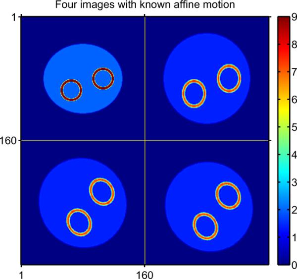
Four true images with anisotropic scale, rotation and translation.

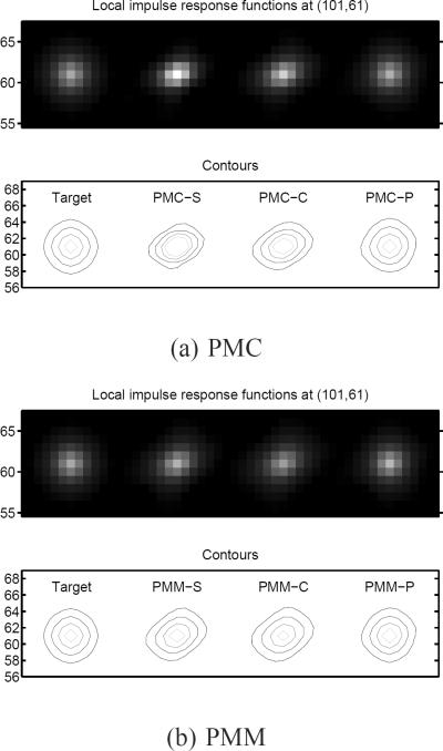
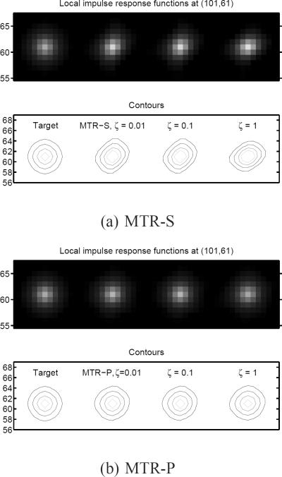
We put an impulse at (101,61) and generated two noiseless projections with original and impulse-added images. We obtained LIRs by subtracting a reconstructed original image from a reconstructed impulse-added image as defined in (13). Figs. 3 and 4 show contour plots of the LIRs of the different MCIR methods and different regularization schemes. Using static spatial regularizers usually led to skewed LIRs (for PMC-S, PMM-S, and MTR-S) due to the spatial-variant noise statistics and the motion. Certainty-based spatial regularizer designs did not alleviate the skewness of LIRs for each MCIR method (PMC-C and PMM-C) and the LIRs of PMC-C and PMM-C do not match the target well. However, our proposed spatial regularization designs of (46) and (49) achieve approximately uniform and isotropic spatial resolution that matches well with our target resolution (PULS estimator) for each MCIR method (PMC-P, PMM-P, and MTR-P with a wide range of ζ). With the proposed regularizer designs, PMC, MTR, and PMM can have approximately the same spatial resolution.

Fig. 3.

LIRs (images and contours) at pixel (101, 61) for different MCIR methods. Our proposed spatial regularization designs can match well with the uniform and isotropic target LIR.

Fig. 4.

LIRs (images and contours) at pixel (101, 61) for MTR. Our proposed spatial regularization designs can match well with the target LIR regardless of ζ while LIRs of MTR-S depend strongly on the ζ values.

The skewed LIRs for conventional regularizers can cause non-uniform estimation bias in small or narrow structures such as small lesions or rings as shown in Fig. 5. These mean images were obtained from the noiseless projections [22]. Fig. 5 (a) shows profiles of the relative image intensity around the right ring of the PMC reconstructed images. Our proposed PMC-P is very close to the target compared to the other regularization methods (PMC-S and PMC-C). The profile of Fig. 5 (b) shows that our proposed regularizer obtained approximately the same quantitative result as that of the target for PMM. Fig. 5 (c) shows that our proposed spatial regularizer (46) approximately achieved the same spatial resolution regardless of ζ, while the spatial resolution of MTR-S changes over ζ.

Fig. 5.

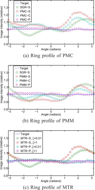
Profiles around the ring on the right of the reconstructed images of PMC, PMM, and MTR (with different ζ values) with different spatial regularizers from the noiseless projection data. Nonuniform and/or anisotropic LIRs lead to non-uniform estimation bias in small or narrow structures such as small lesions or rings. Reconstructed images are shown in supplimentary figures.

We obtained the LIRs and the mean images of different MCIR methods by reconstructing images from noiseless projection data. We also performed 100 noise realizations (regularizer were obtained from each realization) and showed that (result not shown in here) the image from one noiseless projection and the mean image from 100 noise realizations matched very well. They confirm that we can also use the same plug-in technique for MCIR method as that for static case [22] to predict spatial resolution properties.

C. XCAT phantom with nonrigid motion

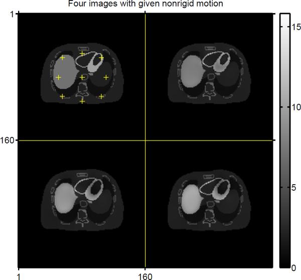
In this simulation, we used XCAT digital phantom [42] with respiratory and cardiac motion to generate 4 volumes with nonrigid motion and selected one slice per each volume (same location) for the 2D simulation. We estimated the motion fields from frame 1 to 2, from frame 1 to 3, and from frame 1 to 4 (for PMM) by using B-spline nonrigid motion estimation [35] and used them as the true motion, leading to the images f₁,⋯ , f₄ shown in Fig. 6. Then, we obtained the other related warps (e.g., motion from frame 4 to 1 for PMC and from 3 to 4 for MTR) by using (54) and the composition of transformations (e.g., T̊_4,3 = T̊_4,1T̊_1,3). Thus, there is no motion model mismatch in this experiment, so that we can focus on the spatial resolution properties.

Fig. 6.

Four XCAT phantom images with nonrigid motion.

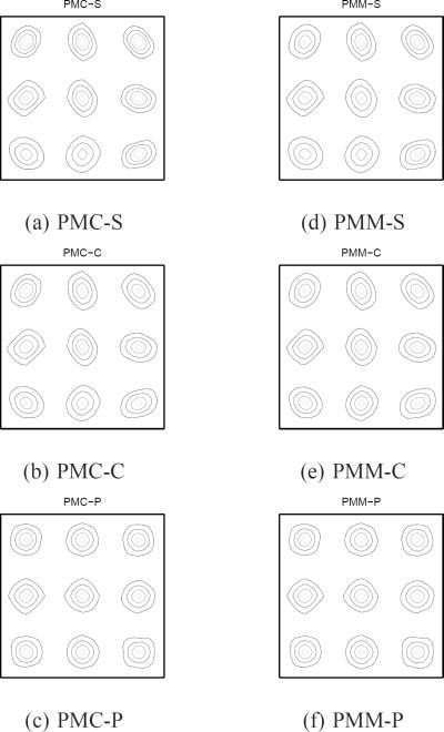
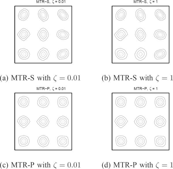
To measure LIRs, we put 9 impulses as indicated in Fig. 6 (+ marks). Fig. 7 shows the LIRs of PMC at the 9 locations. Fig. 7 (a) and (b) show that conventional and certainty-based spatial regularizers lead to skewed LIRs as compared to the Target LIR. However, our proposed regularizer for PMC yielded a good match to the Target LIR as shown in Fig. 7 (c). Fig. 7 (d) and (e) confirm that regularizers that do not strive for isotropic spatial resolution lead to skewed LIRs as compared to the Target LIR. However, our proposed regularizer for PMM shows a good match to the Target LIR as shown in Fig. 7 (f). Fig. 8 shows LIRs of MTR at 9 locations. Fig. 8 (a) and (b) show that conventional regularizer can not achieve the matched spatial resolution to the Target for any ζ value, while our proposed regularizer for MTR produced nearly uniform and isotropic LIRs as in Fig. 8 (c) and (d) for a wide range of ζ values.

Fig. 7.

Contours of LIRs for PMC and PMM. Our proposed PMC-P and PMM-P approaches approximately match with Target spatial resolution for general nonrigid motion.

Fig. 8.

Contours of LIRs for MTR. Our proposed MTR-P approximately matches with Target despite general nonrigid motion and different ζ.

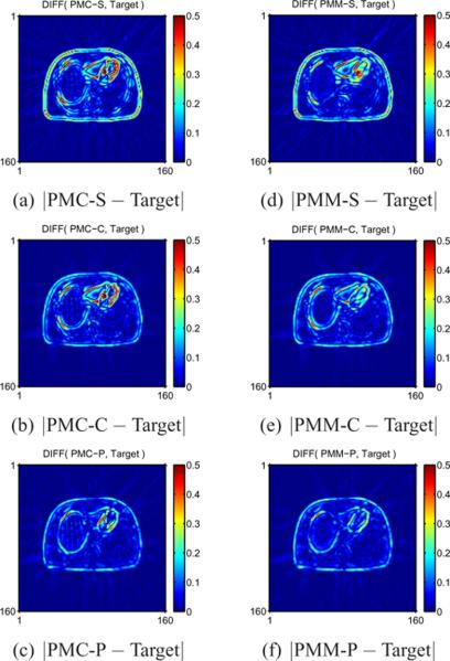
Fig. 9 shows absolute difference images between the mean image for each method and Target. PMC-S differs the most from the Target especially for edges and relatively small structures (near myocardium in our example) in Fig. 9 (a). PMC-C matches somewhat better due to nearly uniform spatial resolution as seen in Fig. 9 (b). Fig. 9 (c) shows that PMC-P best matches the Target. Fig. 9 (d–f) shows similar results for PMM. Similarly, the agreement of PMM from the Target mean image improves as the spatial regularizer encourages uniform and isotropic spatal resolution. Likewise, Fig. 10 shows that our proposed spatial regularizer for MTR yielded the mean images closest to the Target mean image for a wide range of ζ values as shown in Fig. 10 (c), (d), as compared to the results of conventional regularizers in Fig. 10 (a), (b).

Fig. 9.

Absolute difference images between PMC/PMM and Target. PMC-S/PMM-S show severe non-uniform bias near edges or relatively small structures. PMC-C/PMM-C alleviate this bias using nearly uniform spatial resolution and PMC-P/PMM-P performed best by nearly uniform/isotropic spatial resolution.

Fig. 10.

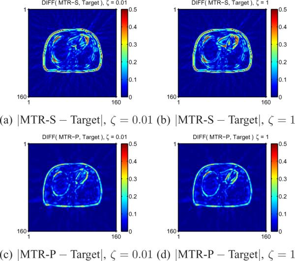
Absolute difference images between MTR and Target. MTR-S with any ζ values show significant non-uniform bias in small or narrow structures such as small lesions or rings, but MTR-P reduces this bias for a wide range of ζ values.

VI. DISCUSSION

The analysis in this paper shows that MCIR for nonrigid (even affine) motion leads to non-uniform and anisotropic spatial resolution properties when one uses conventional static regularizers. We proposed quadratic spatial regularizers that approximately achieve isotropic and uniform spatial resolution for three different MCIR methods for the case of known nonrigid motion. Our proposed regularizers (46) and (49) yielded LIRs that match well with the Target LIR which is isotropic and uniform.

The assumption that the motion is locally affine should be reasonable for any smooth organ motion such as heart and lungs when the time resolution is sufficient (e.g., see [44], [45] for local affine models to approximate cardiac motion). Mathematically, the Taylor approximation of smooth nonrigid motion becomes more accurate as the region of interest (ROI) shrinks. In our analysis, the effective ROI is very small (usually about 2 pixels in each direction) because we focus on each LIR individually. Thus, even for non-affine nonrigid motion, our proposed methods still produced LIRs that match fairly well with the Target LIR. However, this assumption may break for sliding motion such as the motion near the interface between diaphragm and rib cage. For lower resolution modalities like PET or SPECT, this type of motion can still be approximated by smooth motion. For high resolution imaging modalities, treating this sharp sliding motion should be further investigated along with non-quadratic spatial regularizers.

Our analysis assumed `known true motion', but obtaining exact motion from multi-modal imaging systems is challenging due to misregistration between two imaging modalities (e.g. PET and CT) and the non-linear, non-convex nature of image registration problem. We investigated the effect of motion error in our reconstructed images. We reconstructed the simple phantom in Section V-B again, but with 1.7 mm (a half pixel) and 3.4 mm (1 pixel) motion errors in the x-direction deformation. Additionally, we reconstructed PULS image with motion errors by minimizing ${\Vert {\mathit{y}}_{\mathrm{c}}-{\mathit{A}}_{\mathrm{d}}{\mathit{T}}_{\mathrm{c}}{\mathit{f}}_1\Vert }_2^2+\eta {\Vert {\mathit{C}}_0{\mathit{f}}_1\Vert }_2^2$ with respect to f₁ where C₀ is a first-order finite difference matrix for a standard shift-invariant quadratic regularizer. When the motion estimation error was small (1.7 mm), the maximum absolute errors between the reconstructed image and the target image for PULS, PMC-S, and PMC-P were 0.7, 1.9, and 1.1. In this case, the non-uniformity and anisotropy of the bias due to the interaction between Poisson likelihood and regularizers was still significant. However, when the motion estimation error was large (3.4 mm), the maximum absolute errors for PULS, PMC-S, and PMC-P were 1.4, 2.2, and 1.7. The non-uniformity anisotropy of the bias due to the motion error started to become a dominating factor for large motion error. PMM also showed similar tendency. For small motion errors, our proposed regularizers can still reduce the nonuniformity and anisotropy of the bias as expected because ${\tilde{w}}_m$ is slowly varying and we assumed local affine motion (i.e., smooth motion). For large motion errors, MCIR itself may fail to yield images with good quantification accuracy for any regularization method. There is much effort on improving the accuracy of motion estimation by using simultaneous acquisition such as PET-MR, or by using joint estimation of image and motion. The issue of the non-uniform and anisotropic spatial resolution will become increasingly important as the accuracy of the motion estimation in MCIR models continues to improve.

The spatial resolution analysis and regularizer designs in this paper can provide the basis for interesting future work such as analyzing the noise properties of MCIR methods [46] and extending regularization design to 3D PET / CT and to nonquadratic regularizers. It is straightforward to extend this work to 3D cylindrical PET with 6-voxel 3D regularizer [47], which is relevent for 3D PET rebinning methods [48]. Extending this analysis to fully 3D PET or fan-beam CT will be more challenging, just as [23], [27] extended [21], [29], respectively. This analysis can also provide insights into the methods of joint image reconstruction and motion estimation (unknown motion) [7], [8], [11], [13]–[15]. One may use the proposed regularizers in the joint estimation framework by using currently estimated motion instead of using true motion. However, the effect of the proposed regularizer in this case should be further analyzed.

APPENDIX A ADJOINT OPERATOR OF A WARP $\mathcal{T}$

This appendix analyzes the properties of the transpose warp matrix ${\mathit{T}}_{m,n}^{\prime }$ considering its continuous space analogue. Let $T:{\mathbb{R}}^d\to {\mathbb{R}}^d$ denote a spatial transformation with positive Jacobian determinant. Let $\mathcal{X}=L_2\left({\mathbb{R}}^d\right)$ denote the space of (square integrable) images over ${\mathbb{R}}^d$ and define the warp operator $\mathcal{T}:\mathcal{X}\to \mathcal{X}$ by $g=\mathcal{T}f$ if and only if $g\left(\overrightarrow{x}\right)=f\left(T\left(\overrightarrow{x}\right)\right)$ for f, $g\in \mathcal{X}$ and all $\overrightarrow{x}\in {\mathbb{R}}^d$. This appendix determines the adjoint of $\mathcal{T}$, defined as the operator $\mathcal{T}\prime$ that satisfies $\langle g,\mathcal{T}f\rangle =\langle \mathcal{T}\prime g,f\rangle$ for all f, $\langle \cdot ,\cdot \rangle$, where 〈⋅, ⋅〉 denotes the usual inner product on $\mathcal{X}$.

By a simple change of variable $\overrightarrow{y}=T\left(\overrightarrow{x}\right)$, we have

$$\begin{array}{cc}\hfill \langle g,\mathcal{T}f\rangle & =\int g\left(\overrightarrow{x}\right)\left(\mathcal{T}f\right)\left(\overrightarrow{x}\right)d\overrightarrow{x}=\int g\left(\overrightarrow{x}\right)f\left(T\left(\overrightarrow{x}\right)\right)d\overrightarrow{x}\hfill \\ \hfill & =\int f\left(\overrightarrow{y}\right)\frac{1}{\mid \nabla T\left(T^{-1}\left(\overrightarrow{y}\right)\right)\mid }g\left(T^{-1}\left(\overrightarrow{y}\right)\right)d\overrightarrow{y},\hfill \end{array}$$ (51)

where $\mid \nabla T(\cdot )\mid$ denotes the determinant of Jacobian of T. We define an operator ${\mathcal{D}}_T:\mathcal{X}\to \mathcal{X}$ such that

$$g={\mathcal{D}}_{T}fiffg\left(\overrightarrow{x}\right)=\frac{1}{\mid \nabla T\left(\overrightarrow{x}\right)\mid }f\left(\overrightarrow{x}\right),\forall \overrightarrow{x}.$$

Then, by (51), the adjoint operator $\mathcal{T}\prime$ is given by

$$\mathcal{T}\prime ={\mathcal{T}}^{-1}{\mathcal{D}}_T.$$ (52)

Therefore, in continuous space, the adjoint of an invertible nonrigid warp is the product of the inverse of the warp with a diagonal operator based on the local Jacobian determinant of the warp. The discrete approximation that matches (52) is

$${\mathit{T}}_{m,n}^{\prime }\approx {\mathit{T}}_{m,n}^{-1}\mathit{D}\left(\frac{1}{\mid \nabla T_{m,n}\left({\overrightarrow{x}}_j\right)\mid }\right).$$ (53)

Now we use the result (53) and (8) to approximate the transpose of the discrete space matrices ${\mathring{\mathit{T}}}_{m,n}$ in (6) as follows:

$$\begin{array}{cc}\hfill {\mathring{\mathit{T}}}_{m,n}^{\prime }& \approx \left[\mathit{D}\left({\mid \nabla T_{m,n}\left({\overrightarrow{x}}_j\right)\mid }^p\right){\mathit{T}}_{m,n}\right]\prime \hfill \\ \hfill & \approx {\mathit{T}}_{m,n}^{-1}\mathit{D}\left(\frac{1}{\mid \nabla T_{m,n}\left({\overrightarrow{x}}_j\right)\mid }\right)\mathit{D}\left({\mid \nabla T_{m,n}\left({\overrightarrow{x}}_j\right)\mid }^p\right)\hfill \\ \hfill & \approx {\mathit{T}}_{n,m}\mathit{D}\left({\mid \nabla T_{m,n}\left({\overrightarrow{x}}_j\right)\mid }^{p-1}\right)\hfill \\ \hfill & \approx \mathit{D}\left({\mid \nabla T_{n,m}\left({\overrightarrow{x}}_j\right)\mid }^{1-p}\right){\mathit{T}}_{n,m}.\hfill \end{array}$$ (54)

APPENDIX B EQUIVALENT FREQUENCY FORM FOR AFFINE TRANSFORMATION

This appendix analyzes the behavior of a gram matrix or a quadratic regularizer that is sandwiched in between the transpose and forward affine transformation operators such as ${\mathring{\mathit{F}}}_m$ and ${\mathring{\mathit{R}}}_m$ in (16). We consider the continuous-space analogue as follows:

$$\mathring{\mathcal{T}}\prime \mathcal{Q}\prime H\left(\overrightarrow{w}\right)\mathcal{Q}\mathring{\mathcal{T}}$$ (55)

where $H\left(\overrightarrow{w}\right)$ denotes the frequency response with frequency domain variables $\overrightarrow{w}$, $\mathcal{Q}$ is a Fourier transform operator, and $\mathring{\mathcal{T}}$ corresponds to the total activity-preserving affine transform operator that is associated with the affine transform

$$T\left(\overrightarrow{x}\right)=\mathit{L}\overrightarrow{x}+\overrightarrow{d}.$$ (56)

Here, L is a d × d invertible matrix, $\overrightarrow{d}$ is a translation vector, and $\overrightarrow{x}$ is spatial domain coordinates in ${\mathbb{R}}^d$. If $f\left(\overrightarrow{x}\right)$ has Fourier transform $F\left(\overrightarrow{w}\right)$, then the Fourier transform of $\left(\mathring{\mathcal{T}}f\right)\left(\overrightarrow{x}\right)={\mid \nabla T\left(\overrightarrow{x}\right)\mid }^{p}f\left(T\left(\overrightarrow{x}\right)\right)$ is

$$\left(\mathcal{Q}\mathring{\mathcal{T}}f\right)\left(\overrightarrow{w}\right)={\mid \mathit{L}\prime \mid }^{p-1}{e}^{j2\pi \overrightarrow{w}\cdot {\mathit{L}}^{-1}\overrightarrow{d}}F(\left({\mathit{L}}^{-1}\right)\prime \overrightarrow{w}).$$

After multiplying $\left(\mathcal{QT}f\right)\left(\overrightarrow{x}\right)$ by $H\left(\overrightarrow{w}\right)$ and matching a change of variables, the inverse Fourier operator $\mathcal{Q}\prime$ will result in the following continuous function:

$$\int {\mid \mathit{L}\prime \mid }^{p}H(\mathit{L}\prime \overrightarrow{w})F\left(\overrightarrow{w}\right)e^{j2\pi \overrightarrow{w}\cdot (\mathit{L}\overrightarrow{x}+\overrightarrow{d})}d\overrightarrow{w}.$$

Lastly, by Appendix A, an operator $\mathring{\mathcal{T}}\prime$ will change $\mathit{L}\overrightarrow{x}+\underset{‒}{d}$ into $\overrightarrow{x}$ and multiply by ${\mid \mathit{L}\prime \mid }^{p-1}$. Therefore, (55) simplifies to

$$\mathring{\mathcal{T}}\prime \mathcal{Q}\prime H\left(\overrightarrow{w}\right)\mathcal{Q}\mathring{\mathcal{T}}=\mathcal{Q}\prime {(\mathit{L}\prime )}^{2p-1}H(\mathit{L}\prime \overrightarrow{w})\mathcal{Q}.$$ (57)

Note that the translation $\overrightarrow{d}$ does not affect the equivalent frequency response (57). For example, if $H\left(\overrightarrow{w}\right)={\Vert \overrightarrow{w}\Vert }^2={\rho }^2$ in the polar frequency coordinate $(\rho ,\Phi )$, the frequency response of $\mathring{\mathcal{T}}\prime \mathcal{Q}\prime H\left(\overrightarrow{w}\right)\mathcal{Q}\mathring{\mathcal{T}}$ will be ${\mid \mathit{L}\prime \mid }^{2p-1}{\rho }^2{\Vert \mathit{L}\prime \cdot (\text{cos}\Phi ,\text{sin}\Phi )\prime \Vert }^2$.

REFERENCES

- [1].Ritchie CJ, Hsieh J, Gard MF, Godwin JD, Kim Y, Crawford CR. Predictive respiratory gating: a new method to reduce motion artifacts on CT scans. Radiology. 1994 Mar.190(no. 3):847–52. doi: 10.1148/radiology.190.3.8115638. [DOI] [PubMed] [Google Scholar]
- [2].Nehmeh SA, Erdi YE, Ling CC, Rosenzweig KE, Schoder H, Larson SM, Macapinlac HA, Squire OD, Humm JL. Effect of respiratory gating on quantifying PET images of lung cancer. J. Nuc. Med. 2002 Jul.43(no. 7):876–81. [PubMed] [Google Scholar]
- [3].Klein GJ, Reutter BW, Huesman RH. Non-rigid summing of gated PET via optical flow. IEEE Trans. Nuc. Sci. 1997 Aug.44(no. 4):1509–12. [Google Scholar]
- [4].Dawood M, Lang N, Jiang X, Schafers KP. Lung motion correction on respiratory gated 3-D PET/CT images. IEEE Trans. Med. Imag. 2006 Apr.25(no. 4):476–85. doi: 10.1109/TMI.2006.870892. [DOI] [PubMed] [Google Scholar]
- [5].Bai W, Brady M. Regularized B-spline deformable registration for respiratory motion correction in PET images. Phys. Med. Biol. 2009 May;54(no. 9):2719–36. doi: 10.1088/0031-9155/54/9/008. [DOI] [PubMed] [Google Scholar]
- [6].Gravier E, Yang Y, Jin M. Tomographic reconstruction of dynamic cardiac image sequences. IEEE Trans. Im. Proc. 2007 Apr.16(no. 4):932–42. doi: 10.1109/tip.2006.891328. [DOI] [PubMed] [Google Scholar]
- [7].Mair BA, Gilland DR, Sun J. Estimation of images and nonrigid deformations in gated emission CT. IEEE Trans. Med. Imag. 2006 Sep.25(no. 9):1130–44. doi: 10.1109/tmi.2006.879323. [DOI] [PubMed] [Google Scholar]
- [8].Jacobson MW, Fessler JA. Joint estimation of image and deformation parameters in motion-corrected PET. Proc. IEEE Nuc. Sci. Symp. Med. Im. Conf. 2003;5:3290–4. [Google Scholar]
- [9].Qiao F, Pan T, Clark JW, Mawlawi OR. A motion-incorporated reconstruction method for gated PET studies. Phys. Med. Biol. 2006 Aug.51(no. 15):3769–84. doi: 10.1088/0031-9155/51/15/012. [DOI] [PubMed] [Google Scholar]
- [10].Li T, Thorndyke B, Schreibmann E, Yang Y, Xing L. Model-based image reconstruction for four-dimensional PET. Med. Phys. 2006 May;33(no. 5):1288–98. doi: 10.1118/1.2192581. [DOI] [PubMed] [Google Scholar]
- [11].Taguchi K, Sun Z, Segars WP, Fishman EK, Tsui BMW. Image-domain motion compensated time resolved 4D cardiac CT. Proc. SPIE 6510, Medical Imaging 2007: Phys. Med. Im. 2007:651016. [Google Scholar]
- [12].Lamare F, Ledesma Carbayo MJ, Cresson T, Kontaxakis G, Santos A, Cheze LeRest C, Reader AJ, Visvikis D. List-mode-based reconstruction for respiratory motion correction in PET using non-rigid body transformations. Phys. Med. Biol. 2007 Sep.52(no. 17):5187–204. doi: 10.1088/0031-9155/52/17/006. [DOI] [PubMed] [Google Scholar]
- [13].Odille F, Cîndea N, Mandry D, Pasquier C, Vuissoz P-A, Felblinger J. Generalized MRI reconstruction including elastic physiological motion and coil sensitivity encoding. Mag. Res. Med. 2008 Jun.59(no. 6):1401–11. doi: 10.1002/mrm.21520. [DOI] [PubMed] [Google Scholar]
- [14].Chun SY, Fessler JA. Joint image reconstruction and nonrigid motion estimation with a simple penalty that encourages local invertibility. Proc. SPIE 7258, Medical Imaging 2009: Phys. Med. Im. 2009:72580U. [Google Scholar]
- [15].Blume M, Martinez-Möller A, Keil A, Navab N, Rafecas M. Joint reconstruction of image and motion in gated positron emission tomography. IEEE Transactions on Medical Imaging. 2010 Nov;29(no. 11):1892–1906. doi: 10.1109/TMI.2010.2053212. [DOI] [PubMed] [Google Scholar]
- [16].Guérin B, Cho S, Chun SY, Zhu X, Alpert NM, Fakhri GE, Reese T, Catana C. Nonrigid pet motion compensation in the lower abdomen using simultaneous tagged-mri and pet imaging. Medical Physics. 2011;38(no. 6):3025–3038. doi: 10.1118/1.3589136. [DOI] [PMC free article] [PubMed] [Google Scholar]
- [17].Elad M, Feuer A. Restoration of a single superresolution image from several blurred, noisy, and undersampled measured images. IEEE Trans. Im. Proc. 1997 Dec.6(no. 12):1646–58. doi: 10.1109/83.650118. [DOI] [PubMed] [Google Scholar]
- [18].Ng M, Bose N. Mathematical analysis of super-resolution methodology. Signal Processing Magazine, IEEE. 2003 May;20(no. 3):62–74. [Google Scholar]
- [19].Fransens R, Strecha C, Van Gool L. Optical flow based super-resolution: A probabilistic approach. Comp. Vision & Im. Understanding. 2007 Apr.106(no. 1):106–15. [Google Scholar]
- [20].Zibetti M, Mayer J. A robust and computationally efficient simultaneous super-resolution scheme for image sequences. Circuits and Systems for Video Technology, IEEE Transactions on. 2007 Oct.17(no. 10):1288–1300. [Google Scholar]
- [21].Fessler JA, Rogers WL. Spatial resolution properties of penalized-likelihood image reconstruction methods: Space-invariant tomographs. IEEE Trans. Im. Proc. 1996 Sep.5(no. 9):1346–58. doi: 10.1109/83.535846. [DOI] [PubMed] [Google Scholar]
- [22].Fessler JA. Mean and variance of implicitly defined biased estimators (such as penalized maximum likelihood): Applications to tomography. IEEE Trans. Im. Proc. 1996 Mar.5(no. 3):493–506. doi: 10.1109/83.491322. [DOI] [PubMed] [Google Scholar]
- [23].Qi J, Leahy RM. Resolution and noise properties of MAP reconstruction for fully 3D PET. IEEE Trans. Med. Imag. 2000 May;19(no. 5):493–506. doi: 10.1109/42.870259. [DOI] [PubMed] [Google Scholar]
- [24].Stayman JW, Fessler JA. Regularization for uniform spatial resolution properties in penalized-likelihood image reconstruction. IEEE Trans. Med. Imag. 2000 Jun.19(no. 6):601–15. doi: 10.1109/42.870666. [DOI] [PubMed] [Google Scholar]
- [25].Nuyts J, Fessler JA. A penalized-likelihood image reconstruction method for emission tomography, compared to post-smoothed maximum-likelihood with matched spatial resolution. IEEE Trans. Med. Imag. 2003 Sep.22(no. 9):1042–52. doi: 10.1109/TMI.2003.816960. [DOI] [PubMed] [Google Scholar]
- [26].Ahn S, Leahy RM. Analysis of resolution and noise properties of nonquadratically regularized image reconstruction methods for PET. IEEE Trans. Med. Imag. 2008 Mar.27(no. 3):413–24. doi: 10.1109/TMI.2007.911549. [DOI] [PubMed] [Google Scholar]
- [27].Shi HR, Fessler JA. Quadratic regularization design for 2D CT. IEEE Trans. Med. Imag. 2009 May;28(no. 5):645–56. doi: 10.1109/TMI.2008.2007366. [DOI] [PMC free article] [PubMed] [Google Scholar]
- [28].Asma E, Leahy RM. Mean and covariance properties of dynamic PET reconstructions from list-mode data. IEEE Trans. Med. Imag. 2006 Jan.25(no. 1):42–54. doi: 10.1109/TMI.2005.859716. [DOI] [PubMed] [Google Scholar]
- [29].Fessler JA. Analytical approach to regularization design for isotropic spatial resolution. Proc. IEEE Nuc. Sci. Symp. Med. Im. Conf. 2003;3:2022–6. [Google Scholar]
- [30].Chun SY, Fessler JA. Regularization design for isotropic spatial resolution in motion-compensated image reconstruction. Proc. IEEE Intl. Symp. Biomed. Imag. 2011:1500–3. [Google Scholar]
- [31].Unser M, Aldroubi A, Eden M. B-spline signal processing: Part I—theory. IEEE Trans. Sig. Proc. 1993 Feb.41(no. 2):821–33. [Google Scholar]
- [32].Sarrut D, Boldea V, Miguet S, Ginestet C. Simulation of four-dimensional CT images from deformable registration between inhale and exhale breath-hold CT scans. Med. Phys. 2006 Mar.33(no. 3):605–17. doi: 10.1118/1.2161409. [DOI] [PubMed] [Google Scholar]
- [33].Gorbunova V, Lo P, Loeve M, Tiddens HA, Sporring J, Nielsen M, de Bruijne M. Mass preserving registration for lung CT. (ser. Society of Photo-Optical Instrumentation Engineers (SPIE) Conference Series).Society of Photo-Optical Instrumentation Engineers (SPIE) Conference Series. 2009 Feb;vol. 7259 [Google Scholar]
- [34].Asma E, Manjeshwar R, Thielemans K. Theoretical comparison of motion correction techniques for PET image reconstruction. Proc. IEEE Nuc. Sci. Symp. Med. Im. Conf. 2006;3:1762–7. [Google Scholar]
- [35].Chun SY, Fessler JA. A simple regularizer for B-spline nonrigid image registration that encourages local invertibility. IEEE J. Sel. Top. Sig. Proc. 2009 Feb.3(no. 1):159–69. doi: 10.1109/JSTSP.2008.2011116. special Issue on Digital Image Processing Techniques for Oncology. [DOI] [PMC free article] [PubMed] [Google Scholar]
- [36].Skrinjar O, Tagare H. Symmetric, transitive, geometric deformation and intensity variation invariant nonrigid image registration. Biomedical Imaging: Nano to Macro, 2004. IEEE International Symposium.Apr, 2004. pp. 920–923. [Google Scholar]
- [37].Zibetti MVW, Bazán FSV, Mayer J. Determining the regularization parameters for super-resolution problems. Signal Process. 2008;88(no. 12):2890–2901. [Google Scholar]
- [38].Alessio AM, Kinahan PE, Champley KM, Caldwell JH. Attenuation-emission alignment in cardiac pet/ct based on consistency conditions. Medical Physics. 2010;37(no. 3):1911–20. doi: 10.1118/1.3315368. [DOI] [PMC free article] [PubMed] [Google Scholar]
- [39].Hofmann M, Pichler B, Schlkopf B, Beyer T. Towards quantitative pet/mri: a review of mr-based attenuation correction techniques. European Journal of Nuclear Medicine and Molecular Imaging. 2009;36(no. 0):93–104. doi: 10.1007/s00259-008-1007-7. [DOI] [PubMed] [Google Scholar]
- [40].Taguchi K, Kudo H. Motion compensated fan-beam reconstruction for nonrigid transformation. IEEE Trans. Med. Imag. 2008 Jul.27(no. 7):907–17. doi: 10.1109/TMI.2008.925076. [DOI] [PubMed] [Google Scholar]
- [41].Shi H. Ph.D. dissertation. Univ. of Michigan; Ann Arbor, MI: 2008. Fast regularization design for tomographic image reconstruction for uniform and isotropic spatial resolution. 48109-2122, Ann Arbor, MI. [Google Scholar]
- [42].Segars WP, Mahesh M, Beck TJ, Frey EC, Tsui BMW. Realistic CT simulation using the 4D XCAT phantom. Med. Phys. 2008 Aug.35(no. 8):3800–8. doi: 10.1118/1.2955743. [DOI] [PMC free article] [PubMed] [Google Scholar]
- [43].De Pierro AR. A modified expectation maximization algorithm for penalized likelihood estimation in emission tomography. IEEE Trans. Med. Imag. 1995 Mar.14(no. 1):132–7. doi: 10.1109/42.370409. [DOI] [PubMed] [Google Scholar]
- [44].Suhling M, Arigovindan M, Jansen C, Hunziker P, Unser M. Myocardial motion analysis from b-mode echocardiograms. Image Processing, IEEE Transactions on. 2005 Apr;14(no. 4):525–536. doi: 10.1109/tip.2004.838709. [DOI] [PubMed] [Google Scholar]
- [45].Hu M, Penney G, Rueckert D, Edwards P, Figl M, Pratt P, Hawkes D. A novel algorithm for heart motion analysis based on geometric constraints. Medical Image Computing and Computer-Assisted Intervention (MICCAI) 2008;5241:720–728. doi: 10.1007/978-3-540-85988-8_86. [DOI] [PubMed] [Google Scholar]
- [46].Chun SY, Fessler JA. Spatial resolution and noise properties of regularized motion-compensated image reconstruction. Proc. IEEE Intl. Symp. Biomed. Imag. 2009:863–6. [Google Scholar]
- [47].Shi H, Fessler JA. Quadratic regularization design for 3d cylindrical PET. Proc. IEEE Nuc. Sci. Symp. Med. Im. Conf. 2005;4:2301–5. [Google Scholar]
- [48].Defrise M, Kinahan PE, Townsend DW, Michel C, Sibomana M, Newport DF. Exact and approximate rebinning algorithms for 3-D PET data. IEEE Trans. Med. Imag. 1997 Apr.16(no. 2):145–58. doi: 10.1109/42.563660. [DOI] [PubMed] [Google Scholar]
Associated Data
This section collects any data citations, data availability statements, or supplementary materials included in this article.