Theory of active transport in filopodia and stereocilia

Abstract

The biological processes in elongated organelles of living cells are often regulated by molecular motor transport. We determined spatial distributions of motors in such organelles, corresponding to a basic scenario when motors only walk along the substrate, bind, unbind, and diffuse. We developed a mean-field model, which quantitatively reproduces elaborate stochastic simulation results as well as provides a physical interpretation of experimentally observed distributions of Myosin IIIa in stereocilia and filopodia. The mean-field model showed that the jamming of the walking motors is conspicuous, and therefore damps the active motor flux. However, when the motor distributions are coupled to the delivery of actin monomers toward the tip, even the concentration bump of G actin that they create before they jam is enough to speed up the diffusion to allow for severalfold longer filopodia. We found that the concentration profile of G actin along the filopodium is rather nontrivial, containing a narrow minimum near the base followed by a broad maximum. For efficient enough actin transport, this nonmonotonous shape is expected to occur under a broad set of conditions. We also find that the stationary motor distribution is universal for the given set of model parameters regardless of the organelle length, which follows from the form of the kinetic equations and the boundary conditions.

Molecular motor transport in a living cell is one of the most fascinating processes in cellular biophysics. Molecular motors play crucial roles in many elongated organelles, such as neuronal axons (1), flagella (2), filopodia (3), stereocilia (4, 5), and microvilli (4). A naive view of cellular motor transport is that of motor molecules orderly following each other on the substrate and carrying cargo, which they unload at a destination point. However, in reality, motors not only walk, but also diffuse around the cell, randomly binding and unbinding to their substrate filaments and/or cargo. To a large extent these processes are governed by molecular noise. To understand how the motors perform their functions—be it cargo delivery to the growing end of an organelle or creating stresses in a flagellum, or even in artificial systems (6, 7)—it is necessary to know their spatial distribution in these systems.

The spatial distribution of the motors could influence the delivery of building material toward the growing end of a dynamic elongated organelle, such as a filopodium or a stereocilium. In the absence of motors, the length of such organelle is expected to be limited by the slow diffusional delivery of the material to the tip (8). Furthermore, prior computational modeling of simple, conveyor-belt-like transport of monomeric species by molecular motors indicated that specially designed cooperative mechanisms are needed to achieve any appreciable active transport flux (9). Two main reasons for the transport inefficiency are sequestration of cargo by motors and diminution of motor speeds due to clogging of the filamentous bundle by walking motors (9). These “traffic jams” may also be inferred from the corresponding spatial distributions of motors, as discussed below. Another intriguing experimental observation is the localization of the myosin motors at the tips of filopodia (3) and stereocilia (5). All of these findings provide sufficient motivation to look deeper into the spatial distributions of motors and their cargo in actin-based protrusions, and, in particular, to better understand the physical mechanisms which control the delivery of the building materials to the protrusion tips.

The goal of the current work is to find the stationary distributions of motors and their respective G-actin cargo inside cellular protrusions, such as filopodia or stereocilia. We also investigate the way these distributions ultimately regulate the lengths of the corresponding protrusions. In stereocilia, for example, fine regulation of length is important and is clearly coupled to function (10). One expects the lengths of filopodia to also be controlled by cell’s mechanochemical machinery, as seen, for example, in very long filopodia in sea urchin cells (11). Prior calculations showed that diffusional transport is unlikely to provide sufficient G-actin flux to produce such long filopodia (8, 9). In our detailed computational models of motor and G-actin transport in filopodia and stereocilia, the main processes that determine the spatial distributions of motors are (i) directed walking of bound motors on the filaments driven by ATP hydrolysis, (ii) diffusion of free motors in the cytosol, and (iii) the chemical exchange between the bound and free motors. In this work, we have developed an analytical mean-field theory to obtain the stationary concentrations of bound and free motors. It turns out that the mean-field equations for motor profiles are highly nonlinear and cannot be solved numerically using most common approaches, requiring instead a special phase portrait analysis to construct the solution. The resulting motor distributions are in quantitative agreement with our detailed stochastic simulations of growing filopodia and in qualitative agreement with experimental data for Myosin IIIa in stereocilia and filopodia (5). Furthermore, because the motor proteins may carry cargo such as G actins, we also derived the corresponding mean-field equations for the G-actin stationary dynamics. Because G actin’s availability at the protrusion tip determines the corresponding speed of polymerization, the motor-driven G-actin transport may critically influence and, hence, regulate the steady-state lengths of filopodia or stereocilia.

Surprisingly, our mean-field equations indicate that there exists a universal stationary motor profile, which does not depend on the protrusion length. This universality is robust with respect to model parameters or even nature of the elongated enclosed cylindrical environment. We provide a simple explanation for the observed universality of motor concentration profiles. Furthermore, detailed stochastic simulations show that the G-actin concentration profile in filopodium to be nonmonotonic, with a minimum, followed by a maximum (12). Using our mean-field analyses, we suggest a physical explanation that gives rise to the observed nontrivial G-actin distributions. Finally, the stationary motor and cargo distributions may be kinetically difficult to reach for longer filopodia or stereocilia, hence, in the end we discuss the issue of sensitivity to the initial conditions.

Results and Discussion

This section is organized in two parts: the “motor” part and the “actin” part. In the motor part, we present three increasingly realistic mean-field models of motor stationary profile along the tube. By gradually adding complexity we reproduce the results of the stochastic simulations of growing filopodia with the Gillespie algorithm, which is the most comprehensive representation of the complex system dynamics in our work, and thus serves as a check for our mean-field model. Because the resulting motor distribution does not depend on the filopodial length, we use it in the actin part to find the G-actin flux due to active transport, the G-actin concentration profile and the stationary filopodial length set up by the balance of actin fluxes.

Structurally, a filopodium is a bundle of 10–30 actin filaments enveloped by the cell’s plasma membrane (Fig. 1). Filaments are growing at the filopodial tip consuming G-actin monomers (13) delivered from the bulk of the cell by diffusion and possibly motor transport (9). The filaments are pulled back into the cell bulk by special mechanisms inside the cell, in addition, the barbed ends at the tip are pushed by membrane elastic resistance, resulting in a gradual motion of the filaments backwards known as retrograde flow (14). We do not include other regulatory proteins or filament elasticity into the baseline scenario for motor distribution and filopodial growth.

Fig. 1.

A representation of the filopodial model is shown with kinetics scheme of chemical reactions. A filopodium is a cylindrical tube with a bundle of parallel actin filaments inside enveloped by cell’s membrane. The motors can walk on filaments (with speed v determined by forward and backward stepping rates) or diffuse in the solution (with diffusion constant of 5 μm²/s). They can bind and unbind to the filaments (with rates k_on and k_off) and, when on filaments, load, and unload G actin (with rates k_l and k_ul). A loaded motor can detach from the filament simultaneously releasing G actin. Thus, there is no G actin bound to motors in the solution, fulfilling the nonsequestrating regime condition.

Motor Distributions.

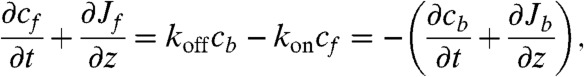
In the motor part of the problem, we consider a cylindrical tube with two types of motors—free and bound—that are subject to two different mechanisms of transport—diffusional and active—respectively. The problem is, therefore, one-dimensional, and we introduce concentrations of free and bound motors, c_f(z) and c_b(z), and write the continuity equations (15)

[1]

where J_f(z) and J_b(z) are forward fluxes for free and bound motors, respectively, and k_off is the unbinding rate of a motor from a site on a filament. For the rate constant of binding between a motor molecule and an F-actin monomer unit, we use the diffusion-limited rate constant, , which translates into rate for a motor to bind to any monomer unit, c_s being the concentration of F-actin monomer units, which are the binding sites, inside the filopodium. To calculate c_s, we count F-actin monomer units in the filopodial volume one-monomer-unit thick, yielding c_s = N/Sδ, where N is the number of filaments, δ is the monomer half-size, and S is the filopodial cross-section. Fick’s law defines J_f(z) = -D∂_zc_f. We assume there are plenty of motors in the cell bulk, which sets a fixed c_f(0) as a boundary condition (BC) at the filopodial base. We can also assume that there is detailed balance between free and bound motors in the cell bulk and, therefore, at the base, and obtain the third BC, k_onc_f(0) = k_offc_b(0). Interestingly, an alternative BC may be adopted without relying on this assumption in case when filaments cease to exist outside of the tube and when comparison with discrete stochastic simulation results is not needed. This BC, which turns out to be c_b(0) = 0, is elaborated in the SI Text, where it is also shown that the choice between the two alternative BCs leads to almost identical results. For the stationary solution of Eq. 1, the total motor flux through a cross-section, corresponding to the integral, J_f + J_b = const, turns out to be zero, J_f + J_b = 0, because of the reflecting BC at the tip. Interestingly, this is the only time the filopodial tip enters the solution for the motors, and it does not introduce the filopodial length as a parameter. Consequently, the stationary motor concentration profiles do not depend on the length. Such universality of motor profile is robust, because it will be also present in other elongated organelles and enclosed cylindrical environments, as long as the system is governed by diffusion and directed random walk, yielding equations of the form Eq. 1 with these BCs. This result is surprising and important.

Phantom Motors Model Failure.

The simplest expression for the bound motor flux is J_b = (v - v_r)c_b, where v is average motor speed generated by ATP hydrolysis steps, and v_r is the retrograde flow speed. Now we have a closed system of equations for the concentrations with stationary solution defined by . This linear set of homogenous ordinary differential equations (ODEs) (phantom motors model, or PMM) has been solved analytically (but with different BCs) to find a motor concentration profile in a stereocilium (15). Our BCs yield an exponential growth of both free and bound motor concentrations toward the tip of a filopodium (dashed lines on Fig. 2). The PMM solution strongly disagrees with the stochastic simulations of the same system. The reason for the failure is that, in the PMM, motors do not interact with each other and can bind onto filaments unlimitedly, regardless of the finite number of binding sites. In reality, c_b(z) is capped by the concentration of binding sites, which in our simulations equals F-actin monomer unit concentration c_s.

Fig. 2.

Comparison of the mean-field analytical models with the stochastic simulation results. The dashed line is the phantom motors model, the solid line is the FFC model, where limited number of binding sites on the filaments is taken into account. Circles are simulation results for c_b, and squares for c_f. Inset zooms into low concentration region to show curves for c_f.

Finite Filament Capacity (FFC).

To account for the saturation of binding sites, one has to make dependent on the number of available binding sites (16). The mean-field equations become nonlinear and can be solved numerically. The results are in a better agreement with the stochastic simulations (solid lines in Fig. 2). Still, the discrepancies are rather notable, especially for the concentration of free motors (Fig. 2, Inset).

Jammed Motors.

To improve the accuracy of the mean-field model, one has to take “clogging” into account. The binding site occupancy prevents a motor from stepping on that site, which leads to the slowdown of the active transport, or “traffic jamming.” To obtain the new equations in a comparatively rigorous fashion, we start with a picture of 1D lattice with biased random walk obeying the Fermi–Dirac statistics (i.e., a motor cannot step to an occupied lattice site) (16). The dynamics of the system (assuming no correlations between lattice site occupancies) are described by an equation similar to the master equation, 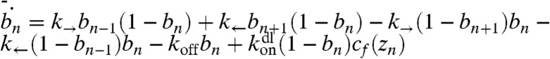, where b_n is the probability that the nth site is occupied, z_n is the spatial location of the nth site, and k_→,k_← are the rates for the forward and the backward steps. The terms for the fluxes resulting from motor steps are obtained by the product of probability that the source site is occupied and probability that the destination site is free multiplied by the step rate. Although the length of motor step is equal to 12 monomers, and there are several filaments inside a filopodium, these subtleties do not influence the continuum limit [c_b(z) = c_sb_n]. The continuum version of the equation coincides with Eq. 1, where J_b = vc_b(1 - c_b/c_s), where v = (k_→ - k_←)l_ss, and l_ss is motor step size. The difference of this expression from the FFC model can be perceived as the modification of the motor speed by the probability that the next site is free. After including the retrograde flow into the final expression for the bound motor flux (J_b = c_b[v(1 - c_b/c_s) - v_r]), we get the equations for the jammed motor model (JMM):

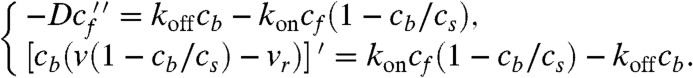[2]

The JMM equations considerably strain the mean-field approach, for instance, they have regions of instability. They cannot be solved with finite differences methods (at least, in a physically meaningful way), but for biologically reasonable parameter values, the mean-field treatment can be saved through the phase portrait analysis of the JMM equations. After using the integral J_f + J_b with the BC, we can rewrite the JMM equations as a set of two first-order ODEs and investigate it as an evolving dynamical system (with z treated as “time”):

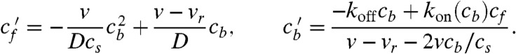[3]

We see that goes to infinity on the singular line 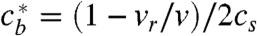except at the point (P) where the numerator in Eq. 3 is also zero. P is therefore the only point where the trajectory can cross the singular line with a physically meaningful result. Still, is undefined in P and will take an arbitrary value when calculated numerically. However, we notice that the system has a nontrivial saddle fixed point Q, when 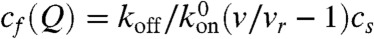and c_b(Q) = (1 - v_r/v)c_s. The point Q corresponds to almost fully saturated filaments (allowing just enough directed motor flux, so that it is fully compensated by retrograde flow) and free motors in chemical equilibrium with the filaments—a situation one would expect far from the filopodial base. This situation is actually observed in the FFC model and the simulations. Thus, as time approaches infinity, a physically meaningful solution should be approaching the point Q along its stable eigenvector, similar to the FFC solution. Shooting backward in time from Q along its stable manifold, we recover the solution down to the singular line of . To finish the construction of the solution for the JMM we integrate Eq. 3 up to the singular line and combine the two parts, thus avoiding the need to cross the singular line.

The solutions for various sets of parameters—k_off, c_f(0), and v—are given in Fig. 3. The JMM gives a very good approximation to the stochastic simulations. We confirmed these stationary solutions, by numerical integration of the time-dependent JMM partial differential equations.

Fig. 3.

Motor concentration profiles inside a filopodium are shown according to stochastic simulations and jammed motors model for various parameter sets (motor affinity to filaments, motor speed, motor concentration). For each set of parameters, the simulations points continue up to the filopodial length from the corresponding simulation. Theoretical curves were computed for all lengths. Inset zooms into low concentration region to show curves for c_f. Circles correspond to simulations, solid lines to the numerical solution of the mean-field theory, and dashed lines to analytical solution of the mean-field theory using the approximation of weakly violated detailed balance.

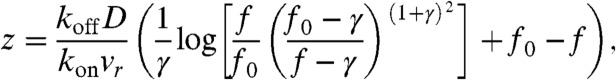
Furthermore, a high-quality closed-form solution to Eq. 2 can be obtained by taking advantage of only weak violation of the detailed balance within any local segment of the tube, and hence, derive a new approximate relation between c_f and c_b, reducing the model to a single ODE that can be solved analytically (see SI Text for more details):

[4]

where f = k_onc_f/k_offc_s, γ = v/v_r - 1, and f₀ = f(0) = k_onc_f(0)/k_offc_s. The solution is given in Fig. 3 as dashed lines and agrees with the full solution very well.

Our results are in qualitative agreement with experiments on delivering of espin1 by Myosin IIIa (M3a) in stereocilia and filopodia, which show gradually growing and saturating M3a concentration profiles, called “drop-like” by the authors due to the characteristic form of their appearance in fluorescence images (5). Similar fluorescence shapes would be expected from the curves in Fig. 3. In particular, the M3a profiles in longer stereocilia have longer saturated regions (bright appearance), which can be explained by our proposed universality of the JMM profiles with respect to organelle length. Indeed, in a longer organelle, a larger part of the same concentration profile would be above the visibility threshold, thus showing up as a larger saturated region.

In our model, traffic jams build up rather close to the organelle base (Fig. 3), which compromises the transport role played by motors if it requires them to be walking far from the base in large numbers. A cell might employ special mechanisms to prevent early jamming, for instance, it could immobilize motors at the organelle tip, effectively removing them from the picture, while they would still show in fluorescence. Localization at the tips is sometimes observed in fluorescence experiments (3, 17). Whirlin, a scaffolding protein, would be one possible candidate for a motor immobilizer. Whirlin was suggested to form complexes with several Eps8 and myosins (17), so if these complexes are anchored at the tip, they could act as myosin sink and prevent jamming.

Apart from jamming, the efficiency of transport may be also decreased by sequestration of the delivered material by motors. Thus, when very fast or very long protrusion is required, alternative processes may be needed. For example, in Drosophila S2 cells, preformed microtubules are pushed from the center of the cell by kinesins and protrude the membrane, forming long processes (18). In axons, cytoskeletal proteins have to be synthesized locally in the growth cone (1, 19), possibly because the need for their consumption is exceeding the active transport delivery limit.

Mathematically, the motor problem is a good example of the need for preliminary qualitative knowledge of the behavior of the system. Solving the FFC model allowed us to construct the JMM solutions, and the simulations provided a consistent check for the mean-field model, as well as motivation to challenge the PM model, which turned out to be inapplicable at greater protrusion lengths.

To put the problem in a larger context, it is well known that stochastic chemical kinetics can be directly mapped onto quantum field theory (20, 21). In this language, the JMM corresponds to coupled bosonic (diffusing motors) and fermionic (walking motors) fields. Earlier works on the problem of motors in a tube have used bosonic–bosonic (PMM) (15) or fermionic–fermionic (22) theories, which in a mean-field approximation yield equations similar to Eq. 2. Our work solves the bosonic–fermionic model, yielding a solution rather different from these prior solutions, and one that matches most closely the physical reality of active transport in protrusions such as filopodia or stereocilia.

Because the stationary motor distribution does not depend on the filopodial length, it can be used as a constant external field to find out how the protrusion length is modified by the active transport, which is discussed next.

Transport of Actin.

To model the active transport of G actin, we allow, in addition to the scheme described above, for motors to load and unload G-actin molecules. We consider the case when motors can only load G actin when they are bound to the filaments, and not when they are free in cytosol. In this way, the problem of sequestration of G actin by motors (9) mentioned above is avoided. The requirement is not completely artificial, as similar mechanisms are known in other motor systems. For instance, kinesin tail can interact with its head domain in an autoinhibitory way (23), possibly preventing important interactions between the head and the microtubule (24). One possible reason for that is saving ATP, but it could also serve to prevent sequestration of the cargo by freely floating motors.

We will now find the filopodial stationary length along with actin concentration profiles. The length is set by the balance of actin fluxes, which should hold in stationary case just like the balance of motor fluxes discussed above (8). There are three transport fluxes of actin: diffusional flux J_D = -D∂_za [where a(z) is the concentration of freely diffusing actin], retrograde flow flux J_r = -Nv_r/Sδ = -v_rc_s, and active transport flux J_AT. The stationary condition is J_D + J_r + J_AT = 0. In addition, at the tip, polymerization converts G actin to F actin, directing the sum of all G-actin transport fluxes (J_D + J_AT) to the retrograde flow. The polymerization flux is J_P = N(k⁺a_tip - k^-)/S, where k^± are the (de)polymerization rates, and in the stationary case J_P = -J_r = J_D + J_AT. In other words, the growth (or retraction) stops, when the concentration of G actin at the tip a_tip provides polymerization flux J_P equal to the retrograde flow flux J_r (8). This condition yields

[5]

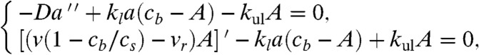
We proceed to finding the stationary length by finding the whole profile a(z) and seeing where a(z) reaches a_tip. G actin can diffuse, load to the motors-on-filaments, and unload, and also be carried forward by them in directed fashion. As discussed in the first section, the stationary motor concentration profile is independent of actin cargo or diffusing G actin, or of the filopodial length. Therefore, from the actin dynamics viewpoint, c_b(z) is just an external stationary field, not a variable. Thus, after taking into account binding site saturation and traffic jamming, the equations for actin yield a set very similar to Eq. 2:

[6]

where A(z) is the concentration of actin carried by motors. The first equation describes the balance of G actin in solution. In addition to diffusion, the G actin in cytosol can be loaded on the motors-on-filaments with the loading rate k_l and unloaded with the rate k_ul. The factor (c_b - A) is the concentration of unoccupied motors-on-filaments. The term in square brackets in the second equation, which describes the fluxes of G actin bound to the motors, is equal to active transport flux J_AT (and differs from J_b in the “motor problem” only by having the factor A instead of c_b). The BCs are also similar to those for motors: (i) At the filopodial base, the concentration of G actin is equal to the bulk concentration in the cell, a(0); (ii) assuming detailed balance of the loading reaction in the bulk and at the base, A(0) = k_la(0)c_b(0)/[k_la(0) + k_ul] (see SI Text for additional discussion); and (iii) like before, we have a conservation law rather than a boundary condition. Finding an integral by summing Eq. 6, we obtain J_D + J_AT = const = -J_r = -v_rc_s, (after applying the actin balance flux condition above to find the constant).

Knowing the motors-on-filaments concentration c_b(z), one is able to solve Eq. 6 numerically. Here we use the solution of Eq. 2, but c_b(z) could in principle be estimated from fluorescence experiments (3, 5, 17) or detailed stochastic computer simulations. Because all the BCs for Eq. 6 are related to the filopodial base (z = 0), the solution can be constructed starting from zero in a straightforward process. We first compute the motor profile distribution c_b(z) from Eq. 2, followed by the G-actin profile distribution, a(z), from Eq. 6, and finally we determine the steady-state filopodial length by finding the position z_tip, where a(z) intersects with a horizontal line drawn at the height a_tip, equal to 2.3 μM for the retrograde flow rate of v_r = 70 nm/s.

From Eq. 6, we predict that the G-actin distribution in a filopodium growing with the help of nonsequestering molecular motor transport is nonmonotonic. This result (also supported by stochastic simulations) is far from obvious, but it can be rationalized through the following arguments. First, assuming J_AT is small at the filopodial base, which is often the case, the slope of a(z) has to be negative there, because of the conservation law, which requires balancing of J_D + J_AT and J_r at the base. On the other hand, one would expect motors to pump the concentration in the tube, so that it grows as a function of distance from the base, as does c_b(z) itself. Thus, empty motors “vacuum up” the diffusing G actin near the base, creating the negative slope of a(z) and transporting these bound molecules farther into the tube. Hence, at some point, a(z) starts to increase, so the slope changes to positive, thus creating a minimum (the minimum may nearly disappear at higher J_AT values at the base, as seen for a red curve in Fig. 4). However, at the same time, the traffic jam builds up, decreasing the efficiency of G actin pumping forward, so after reaching a maximum a(z) starts to drop once again (Fig. 4). Alternatively, the slope of a(z) at the tip has to be negative as well: a(z) > a_tip everywhere inside the filopodium, or it would not be able to grow past the point where a(z) < a_tip. With the requirement of the negative slope both at the base and the tip, it could either be a monotonic decrease, or at least one minimum followed by one maximum. In the absence (or inefficiency) of active transport, we observe the former situation, a nearly linear decrease (SI Text). Fig. 5 shows the magnitude of active G-actin flux J_AT which starts to drop sharply after the region of jamming build up. Interestingly, in some cases, J_AT may be higher at the tip when the unbinding rate, k_off, is increased, which may seem counterintuitive because motors in this case are less processive and spend less time on filaments. On the other hand, the jamming starts further in the tube, increasing transport efficiency in these specific cases.

Fig. 4.

G-actin concentration profiles for different parameter values are shown. Circles represent the results of stochastic simulations and lines are the solutions of Eq. 6 for a(z). All the profiles end when the concentration drops below a_tip (Eq. 5), which is about 2.3 μM for our parameter values.

Fig. 5.

Active transport fluxes for different parameter values are calculated as J_AT(z) = (v[1 - c_b(z)/c_s] - v_r)A(z). Symbols correspond to A(z) and c_b(z) taken from the results of stochastic simulations, and lines are plotted by taking c_b(z) and A(z) from the solutions of Eqs. 2 and 6. Active transport flux decreases after the traffic jam is formed. The retrograde flow flux J_r of 415 molecules per second determines the flux of G-actin monomers, which need to be delivered to the tip at steady state. Dashed line shows the diffusional forward flux of G actin for k_ul = 30 s^-1, k_off = 10 s^-1, [M] = 0.3 μM (corresponding to the black curve on Fig. 4). Active flux is still significant even far from the start of the jam, however, starts to vanish near the tip.

On the left-hand side of the broad maximum in Fig. 4, the J_D is negative and works against the positive J_AT (Fig. 5). After the motor jam builds up, J_AT decreases, so J_D has to increase correspondingly because of the flux balance. Thus the burden of actin delivery transfers from motors to diffusion, so at the tip J_AT can be almost negligible compared to J_D (for one of the parameter sets in Fig. 5, it is 53 vs. 360 molecules per second). Interestingly, J_AT is still considerable far from its maximum, which is very close to the base due to the quick jam development. One of the factors sustaining J_AT is the high value of unjammed motors speed, on the order of one micron per second, which can still deliver noticeable flux even when diminished by an order of magnitude due to jamming. However, it turns out that it is still mainly the diffusion that delivers monomers to the tips of long filopodia for the most of their lengths. The role of active transport can be formulated as that of increasing the concentration gradient for diffusion through locally increasing the concentration near the base, or in the middle of the filopodial tube. From the point of view of actin flux balance, the latter is the same as having a higher “effective” bulk concentration of G actin in a filopodium with no active transport.

The mean-field model for actin is either in quantitative or semiquantitative agreement with the stochastic simulations, depending on model parameters (Figs. 4–6). In terms of stationary length, and positions and heights of G-actin concentration peaks, the discrepancy between the analytical mean-field solution (solid lines) and stochastic simulations (circles) is less than 20–25%. The shapes of the corresponding curves are almost identical, and the discrepancy amounts to scaling the mean-field curves down in both axes. Interestingly, the agreement between mean-field results and stochastic simulations is very accurate for bound species, c_b(z) and A(z), as seen in Fig. 6. Hence, barely noticeable discrepancies for bound species profiles amplify into noticeably larger errors for the cytosolic actin concentration profiles, which in turn determines the filopodial length. This amplification may be understood as a result of pumping current created by motors, which is highly nonlinear. The trend of seeing better agreement for shorter filopodia supports this point of view. Yet another way to formulate the quantitative correspondence between mean-field and simulation results as simple scaling of axes is that noise and fluctuations renormalize the parameters in the mean-field theory (8). In general, if molecular fluctuations are very strong at small protein copy numbers and couple to nonlinear chemical kinetics, the resulting dynamical behaviors might be rather different from the corresponding mean-field predictions (25, 26). In the context of active transport in filopodia, the fluctuations are moderate within certain regime of model parameters, however, the mean-field picture is destroyed when fluctuations become too large in case of other model parameters, as we have seen in the motors part of the problem. In simulations, reaching the steady-state length predicted by the mean-field theory may be a very slow process, taking up to 15 min, sometimes showing more than one distinct stationary or quasi-stationary state (12). Even within the mean-field theory, two different steady states for the same set of parameters are possible (when the first minimum in G-actin profile is lower than a_tip; Eq. 5). In such cases, the filopodial evolution (and length in particular) can be largely defined by the initial conditions for its growth or retraction. Paralleling the stochastic dynamics of a filopodium to navigating an energy landscape (27), one may suggest that this energy landscape is somewhat rugged, similar to that of spin-glasses or heteropolymers, with many kinetic traps appearing as quasi-stationary states.

Fig. 6.

Concentration profiles for actin-on-the-motors A(z) and motors c_b(z) are shown for k_ul = 30 s^-1, k_off = 10 s^-1, [M] = 0.3 μM (corresponding to the black curve on Fig. 4) from analytical solution. The concentration of F-actin binding sites c_s = N/Sδ = 558 μM caps c_b(z), while A(z) is in turn capped by c_b(z). Symbols correspond to A(z) and c_b(z) taken from the results of stochastic simulations, and lines are plotted by taking c_b(z) and A(z) from the solutions of Eqs. 2 and 6.

Conclusion

We have constructed a comprehensive set of mean-field models to describe a possible mechanism of G-actin active transport inside filopodium or stereocilia. The predictions of these equations quantitatively reproduce most of detailed stochastic simulation results and are consistent with a number of experiments on measuring motor fluorescence in actin-based protrusions. The concentration profiles of molecular motors are universal, independent of the protrusion length. This universality is a fundamental property of the problem of motors in a tube, independent of parameters or even the actin-bundle nature of the tubes considered in this work.

According to our model, motors form a traffic jam relatively close to the base of the filopodial tube, which greatly slows down their walking further into the tube. However, local pumping of G actin up to the jamming region can create enough G-actin concentration gradient for diffusion to be able to sustain filopodia several times longer than in the absence of active transport. The pumping is manifested as a nontrivial concentration profile of diffusing G actin, with a minimum followed by a maximum. Hence, despite jamming, motor transport can be quite efficient in producing much longer protrusions. Interestingly, multiple steady-state solutions seem possible under certain combinations of rate constants and species concentrations, which is an issue that should be explored further both experimentally and theoretically. We also observed that kinetic barriers may slow down the approach to the steady state for longer filopodia and stereocilia, hence, finite-time observations may sensitively depend on the initial conditions and could explain some of the variability seen among neighboring protrusions of the same cell.

Materials and Methods

Model Parameters.

We employ the following computational setup (Fig. 1). There are N = 16 actin filaments in the cylindrical filopodial tube with radius R = 75 nm) (28). There are two protofilaments in each filament, so we use half a monomer size δ = 2.7 nm. These values yield a concentration of F-actin monomers in a filopodium c_s = N/πR²δ ≈ 560 μM. G actin is diffusing along the filopodium (D = 5 μm²/s) (29) while its concentration at the filopodial base is maintained by the cell at a constant bulk level a(0) = 10 μM (9, 30, 31). At the tip, G-actin monomers can react with the N barbed ends with the rate k⁺ = 11.6 μM^-1 s^-1 and depolymerize with rate k^- = 1.4 s^-1 (31). Retrograde flow moves the filaments backward with a constant speed v_r = 70 nm/s (14). Myosin motors also diffuse along the filopodium (D = 5 μm²/s), but in addition they can bind to a filament with the rate k_on (for all the binding and on-rates we use the diffusion-limited value of 10 μM^-1 s^-1), unbind with the rate k_off (10–100 s^-1) and perform forward and back steps on filaments with the rates k_→ = 50 s^-1 and k_← = 5 s^-1. In the continuous analytical model, these rates translate into v = (k_→ - k_←)l_ss ≈ 1,400 nm/s (with motor step size l_ss = 32.4 nm). If a motor is bound to a filament, it can also load actin with the rate k_l = 10 μM^-1 s^-1 and unload it with the rate k_ul (10–30 s^-1). To prevent sequestration, when a loaded motor unbinds from a filament, it simultaneously releases its G-actin cargo. Motors cannot step on or bind to an F-actin monomer unit occupied by another motor. Like with G actin, the unbound motors concentration at the base c_f(0) was kept constant at the bulk value (0.1—1 μM).

Stochastic Simulations.

Polymerization, depolymerization, motor stepping, binding and unbinding, actin loading and unloading, and diffusion are treated like chemical reactions with set rates, based on the algorithms elaborated in our prior works (8, 9, 12).

References

- 1.Bagnard D, editor. Axon growth and guidance. Adv Exp Med Biol. 2007;621:5–6. doi: 10.1007/978-0-387-76715-4_4. [DOI] [PubMed] [Google Scholar]
- 2.Riedel-Kruse IH, Hilfinger A, Howard J, Jülicher F. How molecular motors shape the flagellar beat. HFSP J. 2007;1:192–208. doi: 10.2976/1.2773861. [DOI] [PMC free article] [PubMed] [Google Scholar]
- 3.Sousa AD, Cheney RE. Myosin-X: A molecular motor at the cell’s fingertips. Trends Cell Biol. 2005;15:533–539. doi: 10.1016/j.tcb.2005.08.006. [DOI] [PubMed] [Google Scholar]
- 4.Prost J, Barbetta C, Joanny JF. Dynamical control of the shape and size of stereocilia and microvilli. Biophys J. 2007;93:1124–1133. doi: 10.1529/biophysj.106.098038. [DOI] [PMC free article] [PubMed] [Google Scholar]
- 5.Salles FT, et al. Myosin IIIa boosts elongation of stereocilia by transporting espin 1 to the plus ends of actin filaments. Nat Cell Biol. 2009;11:443–450. doi: 10.1038/ncb1851. [DOI] [PMC free article] [PubMed] [Google Scholar]
- 6.Hänggi P, Marchesoni F. Artificial Brownian motors: Controlling transport on the nanoscale. Rev Mod Phys. 2009;81:387–442. [Google Scholar]
- 7.Wang S, Wolynes PG. On the spontaneous collective motion of active matter. Proc Natl Acad Sci USA. 2011;108:15184–15189. doi: 10.1073/pnas.1112034108. [DOI] [PMC free article] [PubMed] [Google Scholar]
- 8.Lan Y, Papoian GA. The stochastic dynamics of filopodial growth. Biophys J. 2008;94:3839–3852. doi: 10.1529/biophysj.107.123778. [DOI] [PMC free article] [PubMed] [Google Scholar]
- 9.Zhuravlev PI, Der BS, Papoian GA. Design of active transport must be highly intricate: A possible role of myosin and Ena/VASP for G-actin transport in filopodia. Biophys J. 2010;98:1439–1448. doi: 10.1016/j.bpj.2009.12.4325. [DOI] [PMC free article] [PubMed] [Google Scholar]
- 10.Manor U, Kachar B. Dynamic length regulation of sensory stereocilia. Semin Cell Dev Biol. 2008;19:502–510. doi: 10.1016/j.semcdb.2008.07.006. [DOI] [PMC free article] [PubMed] [Google Scholar]
- 11.Miller J, Fraser SE, McClay D. Dynamics of thin filopodia during sea urchin gastrulation. Development. 1995;121:2501–2511. doi: 10.1242/dev.121.8.2501. [DOI] [PubMed] [Google Scholar]
- 12.Zhuravlev PI, Papoian GA. Protein fluxes along the filopodium as a framework for understanding the growth-retraction dynamics: The interplay between diffusion and active transport. Cell Adh Migr. 2011;5:448–456. doi: 10.4161/cam.5.5.17868. [DOI] [PMC free article] [PubMed] [Google Scholar]
- 13.Sept D, Xu J, Pollard TD, McCammon JA. Annealing accounts for the length of actin filaments formed by spontaneous polymerization. Biophys J. 1999;77:2911–2919. doi: 10.1016/s0006-3495(99)77124-9. [DOI] [PMC free article] [PubMed] [Google Scholar]
- 14.Kovar DR. Intracellular motility: Myosin and tropomyosin in actin cable flow. Curr Biol. 2007;17:R244–R247. doi: 10.1016/j.cub.2007.02.004. [DOI] [PubMed] [Google Scholar]
- 15.Naoz M, Manor U, Sakaguchi H, Kachar B, Gov NS. Protein localization by actin treadmilling and molecular motors regulates stereocilia shape and treadmilling rate. Biophys J. 2008;95:5706–5718. doi: 10.1529/biophysj.108.143453. [DOI] [PMC free article] [PubMed] [Google Scholar]
- 16.Parmeggiani A, Franosch T, Frey E. Totally asymmetric simple exclusion process with Langmuir kinetics. Phys Rev E Stat Nonlin Soft Matter Phys. 2004;70:046101. doi: 10.1103/PhysRevE.70.046101. [DOI] [PubMed] [Google Scholar]
- 17.Manor U, et al. Regulation of stereocilia length by myosin XVa and whirlin depends on the actin-regulatory protein Eps8. Curr Biol. 2011;21:167–172. doi: 10.1016/j.cub.2010.12.046. [DOI] [PMC free article] [PubMed] [Google Scholar]
- 18.Jolly AL, et al. Kinesin-1 heavy chain mediates microtubule sliding to drive changes in cell shape. Proc Natl Acad Sci USA. 2010;107:12151–12156. doi: 10.1073/pnas.1004736107. [DOI] [PMC free article] [PubMed] [Google Scholar]
- 19.Gumy LF, Tan CL, Fawcett JW. The role of local protein synthesis and degradation in axon regeneration. Exp Neurol. 2010;223:28–37. doi: 10.1016/j.expneurol.2009.06.004. [DOI] [PMC free article] [PubMed] [Google Scholar]
- 20.Lan Y, Wolynes PG, Papoian GA. A variational approach to the stochastic aspects of cellular signal transduction. J Chem Phys. 2006;125:124106. doi: 10.1063/1.2353835. [DOI] [PubMed] [Google Scholar]
- 21.Sasai M, Wolynes PG. Stochastic gene expression as a many-body problem. Proc Natl Acad Sci USA. 2003;100:2374–2379. doi: 10.1073/pnas.2627987100. [DOI] [PMC free article] [PubMed] [Google Scholar]
- 22.Muller M, Klumpp S, Lipowsky R. Molecular motor traffic in a half-open tube. J Phys Condens Matter. 2005;17:S3839–S3850. doi: 10.1088/0953-8984/17/47/014. [DOI] [PubMed] [Google Scholar]
- 23.Howard J, Coy DL, Hancock WO, Wagenbach M. Kinesin’s tail domain is an inhibitory regulator of the motor domain. Nat Cell Biol. 1999;1:288–292. doi: 10.1038/13001. [DOI] [PubMed] [Google Scholar]
- 24.Grant BJ, et al. Electrostatically biased binding of Kinesin to microtubules. PLoS Biol. 2011;9:e1001207. doi: 10.1371/journal.pbio.1001207. [DOI] [PMC free article] [PubMed] [Google Scholar]
- 25.Lan Y, Papoian GA. The interplay between discrete noise and nonlinear chemical kinetics in a signal amplification cascade. J Chem Phys. 2006;125:154901. doi: 10.1063/1.2358342. [DOI] [PubMed] [Google Scholar]
- 26.Modchang C, et al. A comparison of deterministic and stochastic simulations of neuronal vesicle release models. Phys Biol. 2010;7:026008. doi: 10.1088/1478-3975/7/2/026008. [DOI] [PMC free article] [PubMed] [Google Scholar]
- 27.Feng H, Han B, Wang J. Adiabatic and non-adiabatic non-equilibrium stochastic dynamics of single regulating genes. J Phys Chem B. 2011;115:1254–1261. doi: 10.1021/jp109036y. [DOI] [PubMed] [Google Scholar]
- 28.Sheetz MP, Wayne DB, Pearlman AL. Extension of filopodia by motor-dependent actin assembly. Cell Motil Cytoskeleton. 1992;22:160–169. doi: 10.1002/cm.970220303. [DOI] [PubMed] [Google Scholar]
- 29.McGrath JL, Tardy Y, Dewey CF, Meister JJ, Hartwig JH. Simultaneous measurements of actin filament turnover, filament fraction, and monomer diffusion in endothelial cells. Biophys J. 1998;75:2070–2078. doi: 10.1016/S0006-3495(98)77649-0. [DOI] [PMC free article] [PubMed] [Google Scholar]
- 30.Novak IL, Slepchenko BM, Mogilner A. Quantitative analysis of G-actin transport in motile cells. Biophys J. 2008;95:1627–1638. doi: 10.1529/biophysj.108.130096. [DOI] [PMC free article] [PubMed] [Google Scholar]
- 31.Pollard TD. Rate constants for the reactions of ATP- and ADP-actin with the ends of actin filaments. J Cell Biol. 1986;103:2747–2754. doi: 10.1083/jcb.103.6.2747. [DOI] [PMC free article] [PubMed] [Google Scholar]
Associated Data
This section collects any data citations, data availability statements, or supplementary materials included in this article.