Cortical functional connectivity decodes subconscious, task-irrelevant threat-related emotion processing

Abstract

It is currently unclear to what extent cortical structures are required for and engaged during subconscious processing of biologically salient affective stimuli (i.e. the ‘low-road’ vs. ‘many-roads’ hypotheses). Here we show that cortical-cortical and cortical-subcortical functional connectivity (FC) contain substantially more information, relative to subcortical-subcortical FC (i.e. ‘subcortical alarm’ and other limbic regions), that predicts subliminal fearful face processing within individuals using training data from separate subjects. A plot of classification accuracy vs. number of selected whole-brain FC features revealed 92% accuracy when learning was based on the top 8 features from each training set. The most informative FC was between right amygdala and precuneus, which increased during subliminal fear conditions, while left and right amygdala FC decreased, suggesting a bilateral decoupling of this key limbic region during processing of subliminal fear-related stimuli. Other informative FC included angular gyrus, middle temporal gyrus and cerebellum. These findings identify FC that decodes subliminally perceived, task-irrelevant affective stimuli, and suggest that cortical structures are actively engaged by and appear to be essential for subliminal fear processing.

Introduction

The human brain has evolved specialized neural mechanisms for recognizing and processing the emotional expressions of faces (Adolphs 2001). Of particular importance are faces with fearful expressions, which are thought to signal the presence of a source of danger within the environment (Ewbank et al., 2009). It is commonly assumed that threat-related and other biologically salient affective signals are processed automatically, without the requirement of awareness or attention, by a sub-cortical pathway involving the superior colliculus, pulvinar and amygdala (i.e. ‘subcortical alarm’ system, or ‘low road’ hypothesis) (Liddell et al., 2005; Tamietto and de Gelder 2010). However, recent evidence has initiated debate regarding the extent to which these stimuli engage and rely upon cortical networks that are coordinated by sub-cortical regions such as the amygdala and thalamus (i.e. the ‘many roads’ and related hypotheses) (Pessoa and Adolphs 2010).

Evidence arguing for the ‘many-roads’ hypothesis includes anatomical and physiological data in animal models, and behavioral, non-invasive neurophysiology and lesion studies in humans, while data to support the ‘low-roads’ hypothesis in humans has included group neuroimaging studies that have reported greater activation in sub-cortical “alarm” regions for subliminal affective stimuli relative to non-affective stimuli (Liddell et al., 2005) as well as increased covariation of right amygdala with pulvinar and superior colliculus during masked fear conditioning using Positron Emission Tomography (PET) imaging (Morris, Ohman, Dolan 1999) (see de Gelder, van Honk, Tamietto 2011; Pessoa and Adolphs 2010; Pessoa and Adolphs 2011; Tamietto and de Gelder 2010) for detailed reviews and perspectives).

Compared to multivariate pattern analyses which take into account the joint responses (or covariations) of multiple brain regions, group GLM neuroimaging approaches are relatively insensitive due to loss-of-signal from averaging across many sessions and subjects (Cox and Savoy 2003; Norman et al., 2006). An alternative and complementary approach, that could reduce signal-loss and the risk of false positives is to apply multivariate pattern analysis to identify regions of the brain that contain enough information to distinguish between subconscious presentation of biologically salient affective and non-affective stimuli, such as masked fearful and neutral faces.

Although the neural correlates of subliminal (both either task- and task-irrelevant) and threat-related emotional face processing have been extensively investigated using group fMRI studies (Etkin et al., 2004; Fusar-Poli et al., 2009; Kouider et al., 2009; Liddell et al., 2005; Pessoa 2005) as well as group EEG (Kiss and Eimer 2008; Pegna et al., 2011), features of brain activity that contain sufficient information to reliably decode, or “brain-read”, the emotional expression of subliminally processed faces remain to be identified. Identifying such features could be a crucial step towards understanding the subconscious encoding and processing of affective facial stimuli, since these features would have a greater capacity (though less well quantified) for representing distinctions between fear- and non-fear- related cognitive-emotional perceptual states than those previously identified through standard brain mapping approaches (Norman et al., 2006). This is a particularly important goal given that deficits in facial affect processing are thought to underlie psychiatric disorders such schizophrenia, autism, and anxiety (Harms, Martin, Wallace 2010; Machado-de-Sousa et al., 2010).

Decoding, or predicting, a presented stimulus or cognitive state based on brain activity has mostly relied on multi-voxel pattern analysis (MVPA) approaches that take into account the joint, multivariate response of multiple voxels and/or brain regions (see (Norman et al., 2006) for a review). The above approaches have been increasingly applied toward the problem of identifying features of brain activity that can decode explicit emotional face perception (see discussion for a brief review). Statistically significant, albeit modest, decoding accuracies have been demonstrated when using activation (i.e. either instantaneous, time-averaged activity or summary measures of activation such as beta estimates derived from SPM maps) of spatially distributed voxels or regions as input features when predicting the emotional expressions of perceived faces. However, like most other complex brain processes, threat-related stimuli and face perception consists of the coordinated functional connectivity among distributed cortical and sub-cortical brain regions (Ishai, Schmidt, Boesiger 2005; Kober et al., 2008; Vuilleumier and Pourtois 2007). Hence, whole-brain functional connectivity patterns may be more informative than spatial activation patterns when decoding subliminally processed facial emotion.

The current fMRI study employed a blocked design in which subjects were instructed to identify the color of pseudo-colored masked fearful and neutral faces (Etkin et al., 2004). Our primary objective was to test the hypothesis that whole-brain functional connectivity (here Pearson correlation using 40 or 10 time points of fMRI data per example) can discriminate between task-irrelevant and subliminally presented (backwardly masked) fearful and neutral faces, and to identify the functional connections that are most informative in this decoding task. Our secondary objective was to directly assess and compare the decoding ability of correlations that were restricted to regions of the ‘sub-cortical alarm pathway’ and other limbic regions. Finally, we compared the decoding accuracies achieved when using functional connectivity (FC, or pair-wise correlations) vs. activity (i.e. beta estimates from SPM maps). We show that a small subset of connections estimated across the whole-brain (most of which are cortical-subcortical and cortical-cortical that include temporo-parietal regions), can “brain-read” subliminally presented fearful faces with significantly higher accuracies than subcortical-subcortical functional connections restricted to ‘subcortical alarm’ and other limbic regions. In addition, patterns of spatial activity were significantly less informative than whole-brain FC in discriminating between these two conditions. These findings support the notion that the cortex plays an active and essential role in subliminal affect processing, and that this neural processing is sub-served by complex interactions among distributed brain regions.

Materials and Methods

Subjects

A total of 38 (19 female) healthy volunteers (mean age = 29, SD = 6.9) with emmetropic or corrected-to-emmetropic vision participated in the study in accordance with institutional guidelines for research with human subjects. All subjects were screened to rule out severe psychopathology.

Stimuli Presentation Paradigm

Subjects performed a previously reported task (Etkin, Klemenhagen et al. 2004) which consists of color identification of masked and unmasked fearful and neutral faces (Supplementary Fig 1). Results for unmasked conditions, which were used to address separate questions about processing of supraliminal fearful stimuli from those considered here, will be presented elsewhere (submitted).

Stimuli

Black and white pictures of male and female faces showing fearful and neutral facial expressions were chosen from a standardized series developed by Ekman and Friesen (1976). Faces were cropped into an elliptical shape that eliminated background, hair, and jewelry cues and were oriented to maximize inter-stimulus alignment of eyes and mouths. Faces were then artificially colorized (red, yellow, or blue) and equalized for luminosity. The stimulus pool consisted of twelve different i-dentities, each with two expressions (fearful and neutral). Each identity and expression was repeated for each of the three colors (red, yellow and blue.) For the training task, only neutral expression faces were used from an unrelated set available in the lab. These faces were also cropped and colorized as above.

Behavioral task

Each trial consists of fixation cue (200 ms) at the center of the screen, followed by a blank screen (400 ms) and a face presentation (200 ms). Subjects were given 1200 ms to respond with a key press indicating the color of the face. Behavioral responses and reaction times were recorded. All face stimuli were backwardly masked which consisted of 33 ms of a fearful or neutral face, followed by 167 ms of a neutral face mask belonging to a different individual, but of the same color and gender (see Supplementary Figure 1). Each epoch consisted of ten trials of the same stimulus type, but randomized with respect to gender and color, and there were 8 total epochs (four per stimulus type). To avoid stimulus order effects, we used two different counterbalanced run orders. Stimuli were presented using Presentation software (Neurobehavioral Systems, http://nbs.neuro-bs.com), and were triggered by the first radio frequency pulse for the functional run. The stimuli were displayed on VisuaStim XGA LCD screen goggles (Resonance Technology, Northridge, CA). The screen resolution was 800X600, with a refresh rate of 60 Hz. After first entering the scanner, subjects were trained in the color identification task using unrelated, nonmasked neutral face stimuli that were cropped, colorized, and presented in the same manner as described above in order to avoid learning effects during the functional run. Additionally, while still in the scanner and after the main presentation paradigm, subjects were administered a forced-choice test under the same presentation conditions as the functional run and asked to indicate whether they saw a fearful face or not. These data were used to determine d-prime (d’) values using the formula: d’ = z(hit rate) − z(false alarm rate), where z represents transformation to z-scores. After the imaging session, subjects were shown the stimuli again, alerted to the presence of masked faces, and asked to indicate whether they had been aware of fearful faces.

fMRI Acquisition and Analyses

fMRI Data Acquisition

Functional images were acquired on a 1.5 Tesla GE Signa MRI scanner, using a gradient-echo, T2^*-weighted echoplanar imaging (EPI) with blood oxygen level-dependent (BOLD) contrast pulse sequence. Twenty-four contiguous axial slices were acquired along the AC-PC plane, with a 64 × 64 matrix (voxel size 3.125 × 3.125 × 4 mm, TR = 2000, TE = 40, flip angle = 60). Structural data were acquired using a 3D T1-weighted spoiled gradient recalled (SPGR) pulse sequence with isomorphic voxels (1 × 1 × mm) in a 256 × 256 matrix, ~186 slices, TR 34 ms, TE 3 ms.

GLM analysis

Functional data were processed in SPM8 (Wellcome Department of Imaging Neuroscience, London, UK). For preprocessing, the realigned T2*-weighted volumes were slice-time corrected, spatially transformed to a standardized brain (Montreal Neurologic Institute) and smoothed with a 8-mm full-width half-maximum Gaussian kernel. 1st-level regressors were created by convolving the onset of each block (MF, MN, F and N) with the canonical HRF with duration of 20 seconds. Additional nuisance regressors included 6 motion parameters, white matter and csf signal, which were removed prior to time-series extraction.

Node definitions

Brain regions were parcellated according to bilateral versions of the Harvard-Oxford Cortical and sub-cortical atlases and the AAL atlas (cerebellum) and were trimmed to ensure no overlap with each other and to ensure inclusion of only voxels shared by all subjects (Figure 2A top, Supplementary Figure 2A). For each subject, time-series across the whole run (283 TRs) were extracted using Singular Value Decomposition (SVD) and custom modifications to the Volumes-of-Interest (VOI) code within SPM8 to retain the top 2 eigenvariates from each region. This resulted in a total of 270 nodes with an associated time course (i.e. eigenvariates) and ROIs (spatial eigenmaps) from the 135 initial atlas-based regions (Figure 2A bottom, Supplementary Figure 2B). For anatomical display purposes, ROI locations were defined in MNI coordinates at the peak value of each eigenmap averaged over all subjects. We used SVD (as opposed to simply the mean signal in each atlas-based region) to avoid inadvertently ignoring and/or averaging away important variation within (particularly larger) regions.

Fig. 2. Large-scale functional connectivity discriminates between processing of masked fearful and neutral faces.

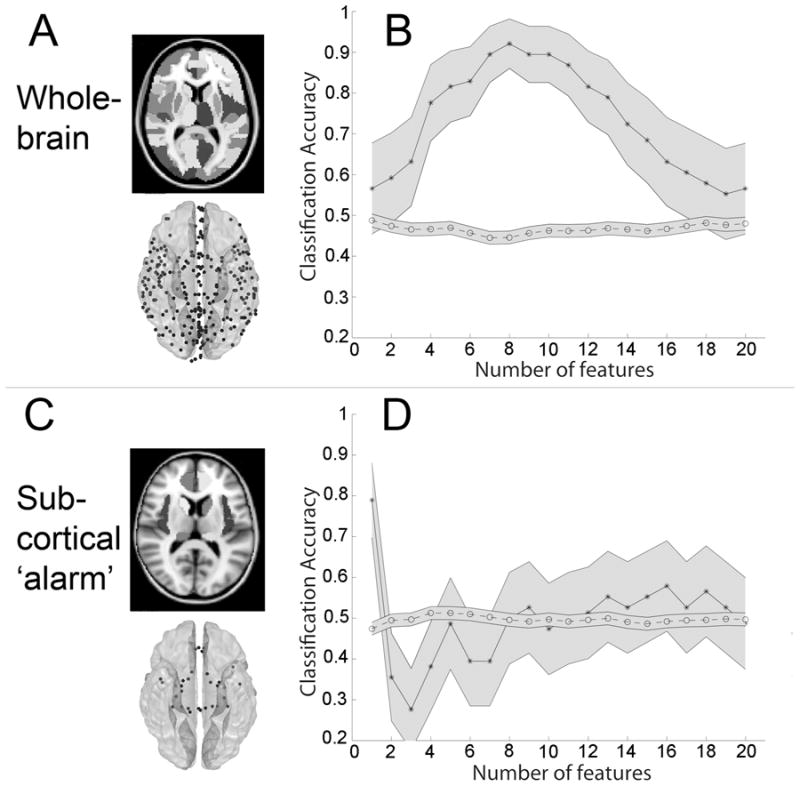
(A) Slice depicting anatomic parcellation scheme and average node locations (see also methods and Supplementary Figure 2A–B). (B) Decoding accuracy when classifying MF vs. MN as a function of the number of features (1 to 20) ranked in descending order by their absolute t-score. Maximum accuracy for MF vs. MN classification (92%, p < 0.0001) was achieved when learning was based on the top 8 features in each training set. (C) Discriminating subliminal fear using large-scale connectivity among “subcortical alarm” and other limbic regions. Bilateral masks for hippocampus, dorsal and ventral amygdala, insula and caudate, anterior cingulate, pulvinar and superior colliculus were defined using WFU_pickatlas with the exception of superior colliculus and locus ceruleus, which were manually drawn using FLSview (amygdala was manually separated into dorsal and ventral regions along z=0). These regions produced 32 nodes (depicted in D, bottom) and 496 total features. More slices of these regions and average MNI locations for each node are listed in Supplemental Figure 2C and Supplementary Table 2 respectively. (D) Classifications using pairwise correlations among the above regions as features and were performed similarly to those presented in Figure 2B. MF vs. MN classification reached a peak accuracy of 79% (p < 0.0001) at 1 feature. Mean accuracy scores for randomly permuted data are plotted along the bottom, and shaded grey regions represent 95% CI. (Because we permuted labels 50 times for each top N features, the total sample size for each null distribution was 50 times greater than for the real distribution, and hence CI are smaller.)

Functional connectivity networks for subliminal fearful and neutral face processing

For each subject, functional connectivity matrices (i.e. where cell i,j contains the Pearson correlation between region i and region j) were generated for masked fearful (MF) and masked neutral (MN) conditions. Time series were high-pass filtered (periods above 128 s were removed) and adjusted for effects-of-interest (i.e. effects of session mean, white matter and csf signal were removed), and were then segmented and concatenated according to conditions of interest (40 total time points per condition, incorporating a lag of 2 or 3 s from the start of each block) before generating the correlation matrices. We concatenated time courses from each of the four 4 blocks per condition in order to maximize the quality of the estimated FC measures (i.e. decrease the noise in the pairwise correlations). Fisher’s R to Z transform was then applied to each resulting correlation matrix. Finally for the binary classification of interest (i.e. MF vs. MN), correlation matrices were demeaned with respect to the average between the two conditions in order to remove the effects of inter-subject variability. The lower triangle of the above preprocessed correlation matrices (38 subjects X 2 conditions total) were then used as input features to predict viewed stimuli.

Pattern analysis of large-scale functional connectivity to predict subliminal (and implicit) fear perception

Support vector machines (SVM) are pattern recognition methods that find functions of the data that facilitate classification (Vapnik 1999). During the training phase, an SVM finds the hyperplane that best separates the examples in the input space according to a class label, where ‘best’ is defined by constraints (maximum margin and the slack variables that allow for a soft margin). The SVM classifier is trained by providing examples of the form <x,c>, where x represents a spatial pattern and c is the class label. In particular, x represents the fMRI data (pattern of correlation strengths) and c is the condition or group label (i.e. c = 1 for MF and c = −1 for MN). Once the decision function is determined from the training data, it can be used to predict the class label of new test examples.

For all binary classification tasks, we applied a linear kernel SVM with a filtering feature selection based on t-test and leave-two-out cross validation (LTOCV). There were 38 examples for each condition (2 from each subject, 76 total). During each iteration of 38 rounds of LTOCV, both examples (1 from each class) from one subject were withheld from the dataset and 1) a paired t-test was performed over the remaining training data (N=37 in each group) 2) the features were ranked by absolute t-score and the top N were selected 3) these selected features were then used to predict the class of the withheld test examples during the classification stage. The full feature set for each example consisted of 36,315 correlations.

If the classifier predicted all trials as positive or negative, the resulting accuracy would be 50% since the number of examples are equal for each class. We therefore report classification accuracy (number of true positives and negatives over all trials) vs. number of included features that have been ranked by their t-score. We first examined whole-brain FC based on concatenated time-series and plotted classification accuracy vs. every 5 features from the top 1 through 200 (the maximum number was chosen heuristically based on (Dosenbach et al., 2010)). Other than a peak near 10 features, accuracies hovered near 50%. Therefore we changed the range to every single feature from top 1 through 20. For sub-cortical ‘alarm’ FC we used the same initial range (5 to 200) to confirm that accuracies also hovered near 50% beyond 10 features, and then plotted results using 1 to 20 features as above. We also plotted the null distribution and assessed the significance of peak decoding results by computing the frequency in which actual values surpassed those from null distributions derived by randomly permuting class labels. To derive this null distribution, class labels within each pair conditions from each subject were randomly flipped with a probability of 0.5 over 10000 iterations (top N features at which peak accuracy was achieved) or 50 iterations (for plots at each number of included features). Uncorrected p-values were reported, and unless otherwise stated, p-values were also corrected at p<0.05 for multiple comparisons using Bonferroni procedure. For plots, 95% Confidence Intervals (95% CI) of the accuracy score were calculated using the normal approximation interval of the binomial distribution: (p±Zc*√[p(1−p)/n], where p=TP+TN/(TP+FP+TN+FP), Zc=97.5 percentile of a standard normal distribution, and n=sample size. This formula was used as it is the simplest and most commonly used to approximate confidence intervals for proportions in a statistical population, and because there was adequate sample size and proportions were not extremely close to 0 or 1 (Newcombe 1998).

For SVM learning and classification we used the Spider v1.71 Matlab toolbox (http://people.kyb.tuebingen.mpg.de/spider/) using all default parameters (i.e. linear kernel SVM, regularization parameter C=1). We attempted SVM learning using a radial basis function kernel and sigma=2 as suggested previously (Dosenbach et al., 2010), but in general performance results were no better than a linear kernel SVM. Thus all analysis used default parameters. Graphical neuro-anatomical connectivity maps were displayed using Caret v5.61 software (http://brainvis.wustl.edu/wiki/index.php/Caret:About).

For assessing the significance of the differences between decoding results (i.e. whole-brain FC as features vs. subcortical FC) we used the Accurate Confidence Intervals MATLAB toolbox for assessing whether the parameter p (probability of correct prediction) from two independent binomial distributions was significantly different (http://www.mathworks.com/matlabcentral/fileexchange/3031-accurate-confidence-intervals). Briefly, these methods search for confidence intervals using an integration of the Bayesian posterior with diffuse priors to measure the confidence level of the difference between two proportions (Ross 2003). We used the code prop_-diff(x₁,n₁,x₂,n₂,delta), (available from the above website) returning Pr(p₁–p₂-δ), where x₁, n₁, x₂, n_2, are number of correct responses and total predictions in two distributions being compared, and delta (zero in our case) is the full hypothesis difference between the probabilities.

Results

Behavioral results

The average response rate in the color discrimination task was 98% (stdev=4.6%), mean accuracy was 97% (stdev=3.5%), and mean reaction time was 0.65 s (stdev=0.12), indicating that subjects performed the task as instructed. In the task used to determine d’ scores (see methods), twelve subjects reported that no masked fearful face had been presented). In the remaining subjects, mean observed d’ score was 0.13, std = 0.35, and the max was 0.71 (~65% accuracy). A one-sample t-test confirmed these scores were not significantly different than zero (p=0.07). We also included the twelve subjects who only responded with misses and correct rejections. In order to do so we had to slightly adjust their hit rate and false alarm from 0 and 1 to 0.01 and 0.99 respectively, since the z-transform is undefined at 0 and 1. These subjects’ d’ scores thus all became -4.65, and when they were included in a new one-sample t-test the overall scores were significantly negative (p=0.0006). Taken together, the above results indicate that backward masking was successful.

Discriminating between subliminal processing of fearful and neutral faces with whole-brain patterns of functional connectivity

We applied atlas-based parcellation and computed pair-wise correlations between 270 cortical and sub-cortical brain regions, or nodes, using 40 total time points of fMRI data that were segmented and concatenated from two conditions; task-unrelated viewing of backwardly masked fearful (MF) and neutral (MN) faces (Figure 1). This resulted in 36,315 total functional connections (z-transformed Pearson correlations) for each condition (MF, MN). The atlas-based parcellation scheme and average node locations are shown in Figure 2A and Supplementary Figure 2, while MNI coordinates and labels corresponding to each node are listed in Supplementary Table 1.

Fig. 1. Data analysis scheme.

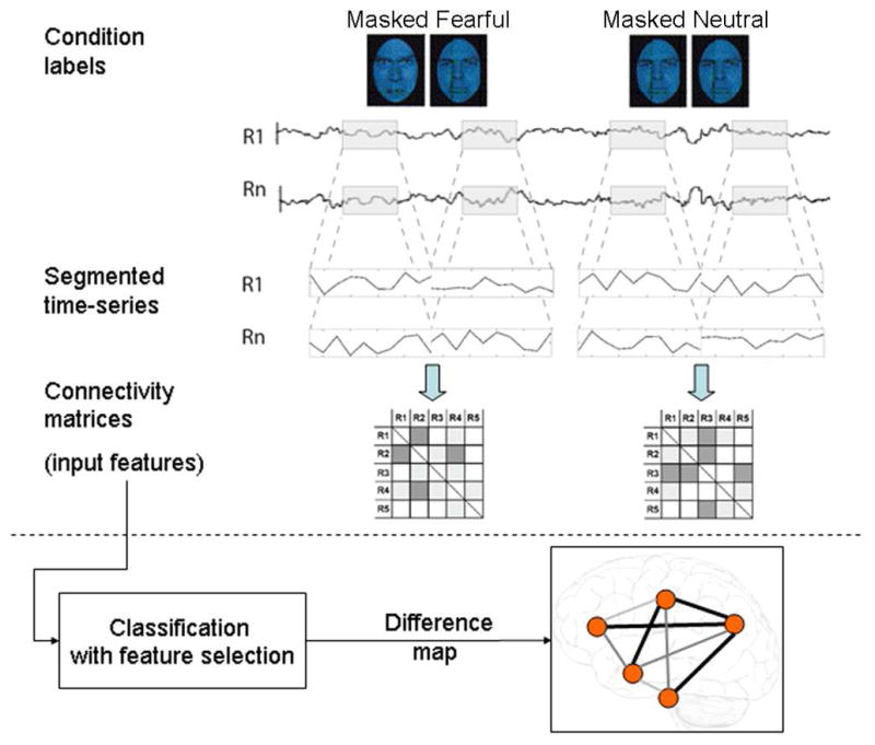
Time series from each condition (masked fearful and masked neutral, MF and MN) and for N regions (R1 though RN) were segmented from each subject’s whole run and concatenated (concatenation of two blocks for each condition shown in figure). Each event (stimulus presentation) consisted of 33 ms presentation of the backwardly masked face followed by 167 ms of a neutral face of different identity, and there were 10 events spaced 2 s apart in each block. There were four 20 second (10 scan) blocks of each condition; hence each example was comprised of 40 time points per condition per subject. For each example, correlation matrices were estimated in which each off-diagonal element contained Pearson’s correlation coefficient between region i and region j. The lower diagonal of each of these matrices were used as input features in subsequent classifiers that learned to predict the example (i.e. MF or MN) based on their observed patterns of the correlations. Here, we used a filter feature selection based on t-scores in the training sets during each iteration of leave-two-out cross validation. The difference map consists of the set of most informative features (those that are included in the most rounds of cross-validation and have the highest SVM weights.)

The extent to which a subset of these functional connections could decode, or predict, the conditions from which they were derived was quantified by submitting them as features into a linear kernel SVM pattern classifier using filter feature selection based on the t-score of each feature (functional connectivity) in each training set. Decoding accuracies for subliminal fearful vs. neutral classifications (MF vs. MN) were plotted against the number of included features (ranked in descending order by t-score) in order to approximate the number of informative features relevant to the emotional expression of the facial stimulus. If there is a true signal present in the data, we expect that there should be an initial rise in accuracy as more informative features are added to the feature set, and a dip in accuracy as less informative features (i.e. noise) are added to the feature set. This is indeed what we observed. For MF vs. MN classification, accuracy reached a maximum of 92% (p < 0.0001) when learning was based on the top 8 features in each training set (Figure 2B).

When extracting only one eigenvariates per region, maximum accuracy reached 87% at with the top 4 features (data not shown). When computing classification accuracy when only using the second eigenvariate from each atlas-based region, classification reached a maximum accuracy of 78% at one feature (data not shown). The highest classification accuracy (92%, Figure 2B) was achieved when using both first and second eigenvariates from each atlas-based region, indicating that correlations between the first and second eigenvariate (of different regions) made substantial contributions in decoding subliminal fear. We note that this means that in some instances node 2 of a particular region showed functional connectivity that differentiated between conditions and node 1 of the same region had no differential connectivity. This is possibly due to the fact that atlas-based parcellation is somewhat arbitrary, and that large regions encompassed many other functionally relevant subregions which were not included when only extracting the top eigenvariate. Another possible reason is that for many regions, the first eigenvariate may reflect artifact global or mean grey matter signal (while white matter and csf signal were regressed out from nodes’ time-series, global and mean grey matter signals were not).

Although time-series were high-pass filtered and white-matter and csf signal was removed, it is possible that slow frequency drifts (just below periods of 128 s and manifesting within global grey matter signal) remained, and that these drifts could have artificially increased the variance in (and hence affect the correlation between) the concatenated time series. Given our use of counterbalanced designs, this effect should not have been enhanced in the concatenated time-series from one condition over the other, and hence any differences in FC between conditions should be attributed to differences in stimulus features of subliminally presented faces, not the above-mentioned potential artifacts. Nevertheless, we explicitly tested the extent to which differences in the mean and variance of signal across the session blocks (stemming from condition-related differences, low frequency artifact drift or physiological noise, etc.) may have contributed to the correlations that discriminated between the two conditions of interest. For this we compared classification rate of the top 8 features listed in table 1 using their original correlations vs. recomputed correlations whereby time points within each segment were first converted to z-scores prior to concatenation. This step resulted in only a 2% decrease in classification rate (97% without z-scoring, 95% with z-scoring) for these eight features, indicating that the effects of concatenation on the computed correlations were minimal.

Table 1. MF vs. MN, Top 8 features.

Fset column indicates the number of rounds of cross-validation in which that feature was included in the feature set.

Edge label	Mean R (MF)	Mean R (MN)	T-value	SVM weight	FSet
Right_Precuneous_Cortex_PC2 - Right_Amygdala_PC1	0.08955	−0.06	4.6834	2.0789	38
Left_Middle_Temporal_Gyrus_temporooccipital_part_PC1 - Cerebelum_6_L_PC1	0.12274	−0.0288	5.1352	2.0298	38
Right_Angular_Gyrus_PC2 - Cerebelum_8_R_PC2	0.10755	−0.0287	4.5288	1.977	33
Right_Temporal_Fusiform_Cortex_anterior_division_PC1 - Left_Middle_Temporal_Gyrus_posterior_division_PC2	−0.1005	0.07104	−4.5939	−1.739	38
Right_Supramarginal_Gyrus_posterior_division_PC1 - Right_Middle_Temporal_Gyrus_posterior_division_PC1	0.08535	−0.0833	4.8447	1.6768	38
Right_Middle_Temporal_Gyrus_posterior_division_PC1 - Right_Angular_Gyrus_PC1	0.14826	0.01222	4.4637	1.515	29
Left_Middle_Temporal_Gyrus_posterior_division_PC1 - Left_Cingulate_Gyrus_anterior_division_PC1	0.15493	0.00869	4.4121	1.3089	22
Right_Amygdala_PC2 - Left_Amygdala_PC1	−0.0564	0.06443	−4.6623	−1.1944	38

Discriminating between MF and MN faces using functional connectivity among ‘subcortical alarm’ system and other limbic regions

Previous work in animal models confirms a sub-cortical “alarm” pathway for fast and subliminal fear processing through the superior colliculus, pulvinar and amygdala (Tamietto and de Gelder 2010). However, direct evidence for this pathway in humans is sparse (Pessoa and Adolphs 2010). We tested whether functional connectivity among these and other sub-cortical and limbic ROIs could discriminate between masked threat-related and neutral facial stimuli using masks for left and right dorsal and ventral amygdala, pulvinar, insula, anterior cingulate, hippocampus, caudate and bilateral superior colliculus and locus ceruleus (Figure 2C). Classifications used pair-wise functional connections amongst the above regions (32 nodes, 496 total features) and were performed as above (Figure 2B, right panel). In contrast to peak decoding results obtained when using functional connections across the whole-brain (92%), MF vs. MN discrimination using features restricted to ‘sub-cortical alarm’ and limbic regions only reached a peak accuracy of 79% (p < 0.0001) at the top 1 feature (Figure 2D, R Caudate – R Insula, MF > MN T-value=3.68). Thus classification accuracy using only subcortical ‘alarm’ and limbic ROIs was less effective than using ROIs throughout the whole-brain.

To ensure that results were not degraded by imperfections in registration that would particularly affect smaller subcortical structures such as superior colliculus, an additional analysis was performed which included larger subcortical structures. All these ROIs were a subset of those included in the whole-brain analysis conducted above, which were parcellated according to the Harvard Oxford Subcortical Atlas. These included bilateral thalamus, midbrain and pons (which were derived from the whole brain-stem ROI, and are depicted in Fig 2, left panel, z=0), amygdala, hippocampus, pallidum, putamen, anterior and posterior parahippocampal gyrus, caudate and nucleus accumbens. In addition, the top four (instead of two) eigenvariates were extracted from each region, resulting in 80 total nodes. Peak classification accuracy (82%, p < 0.0001) was achieved when selecting two features, which included the previously identified bilateral amygdala functional connection (Table 1, last row) and a connection between amygdala (second eigenvariate) and pons (third eigenvariate), which increased during fear and was included in 36/38 rounds of cross-validation (data not shown).

Discriminating between MF and MN faces with patterns of activation

To compare the information content of patterns of functional connectivity (i.e. functional connections used above) vs. patterns of neural activity, we also performed MF vs. MN classification using beta estimates, which are scaling factors estimated from the General Linear Model and can be considered a summary measure of activation to each condition. Our primary goal was to assess the relative classification performances when using “betas” as features under “best-case scenario” conditions. Thus we employed a single, biased feature-selection step in which features (voxels) were chosen based on an F-test conducted over the entire data set. An inclusion mask was defined from an F-test of the contrast MF > MN (p < 0.05, k=30: 6,248 total features, Figure 3A, yellow). Accuracies were plotted against the number of included features ranging from 1 to 6000. In spite of biased feature selection, MF vs. MN classification only reached a maximum of 79% accuracy (p<0.0001, Figure 3B).

Fig. 3. Discriminating subliminal fear using beta estimates as features.

(A) Features for MF vs. MN classification were selected based on an F-test of the contrast MF>MN (p<0.05, k=30: 6,248 total features), respectively. (B) Classifications were performed similar to main analyses in the text but over the range of 1 to 6000 ranked features. Note that feature selection was biased by using a single mask based on the F-test conducted over the complete data set. In spite of this, MF vs. MN classification only reached a peak accuracy of 79% (p< 0.0001, not significant after Bonferroni correction for multiple comparisons) with top 8 to 21 features. Shaded grey region represents 95% CI. Brain images are displayed using Neurological convention (i.e. L=R).

In addition to using whole-brain beta maps, we derived beta weights using the same summary time courses (eigenvariates) that were extracted and used to compute pairwise FC (270 total betas per condition per subject). For this, the GLM analysis was kept the same as above except that previously included nuisance regressors (6 motion, mean white and mean csf) and a low-pass filter were not included, since they were already removed from the time courses during extraction. Resulting estimated beta weights were then used as features to predict fearful vs. neutral faces using the exact same procedure when using whole-brain FC. For this analysis feature selection was unbiased, using filter feature selection during leave-two-out cross validation. Peak accuracy of 71% (p=0.0036 uncorrected, not significant after Bonferroni correction for multiple comparisons) was achieved at top 5 features.

Top FC features that discriminated between MF and MN faces

We formally compared the “information content” of whole-brain FC vs. subcortical alarm FC and whole-brain betas when used as features in predicting MF vs. MN faces. For this we tested for significant differences between the maximum classification accuracies achieved for whole-brain FC vs. the other two (see methods). The maximum accuracy for whole-brain FC (92%) was significantly greater that maximum accuracy achieved with sub-cortical ‘alarm’ FC (79%) (p = 0.01) as well as the peak accuracy achieved whole-brain beta values with biased feature selection (79%) (p=0.01).

Anatomical display of the top 8 overall whole-brain FC features that discriminated between MF and MN conditions revealed functional connections among regions in right middle temporal gyrus, angular gyrus, amygdala, cerebellum, precuneus and anterior cingulate (Figure 4, Table 1). The connection that carried the most weight in the linear SVM classifier was between right amygdala and precuneus, which exhibited a greater correlation in the MF vs. MN condition. The most informative feature when decoding using subcortical ‘alarm’ and limbic regions is listed in Supplementary Table 3.

Fig. 4. Most informative overall features that discriminated between MF and MN faces.

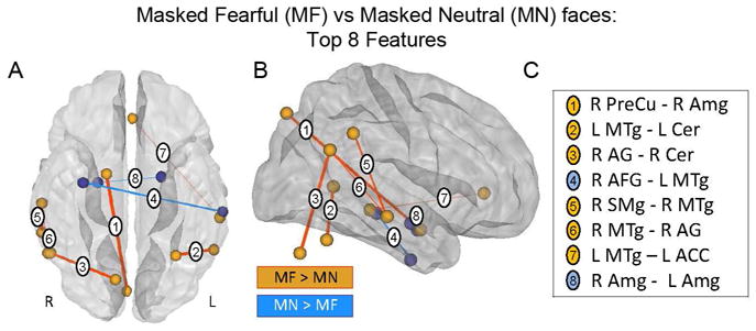
Ventral (A) and right lateralized (B) anatomical representation of the top 8 overall features. Red indicates correlations that are greater in MF, and blue represents correlations that are greater in MN. For display purposes, the color of each sphere is set according to the sign of the sum of the SVM weights of each node’s connections; positive sign, red, MF > MN and negative sign, blue, MN > MF, and the thickness of each connection was made proportional to its weight. (C) Table of top 8 overall features depicted in panels A and B. All features were first ranked according to the number of rounds of cross-validation in which they were included during the filter feature selection (38 maximum). The top 8 from this list were then ranked according to the absolute value of their averaged weight in the Support Vector Machine (SVM). Abbreviations: R PreCu = Right Precuneous Cortex PC2; R Amg = Right Amygdala PC1 (connection 1) and PC2 (connection 8); L Amg = Left Amygdala PC1; L MTg = Left Middle Temporal Gyrus temporooccipital part PC2 (connection 4) and PC1 (connection 7); L Cer = Cerebelum 6 L PC1; R AG = Right Angular Gyrus PC2; R Cer = Cerebelum 8 R PC2; R AFG = Right Temporal Fusiform Cortex anterior division PC1; R SMg = Right Supramarginal Gyrus posterior division PC1; R MTg = Right Middle Temporal Gyrus posterior division PC1; LACC = Left Cingulate Gyrus anterior division PC1.

Discussion

The current work demonstrates that patterns of functional connectivity (pair-wise cortical-cortical and subcortical-cortical functional connections) contain sufficient information to decode the emotional expression of task-irrelevant, subliminally presented faces. The connections that discriminated between subliminally presented fearful and neutral faces included amygdala, temporo-occipital and temporo-parietal regions, with the majority of connections involving the posterior and anterior middle temporal gyrus (in the vicinity of the superior temporal sulcus, STS). This is consistent with models and studies of emotional face recognition that identify the STS and middle temporal gyrus as a primary neural substrate for suprathreshold processing of the emotional expression of faces (Haxby, Hoffman, Gobbini 2002; Sabatinelli et al., 2011; Said et al., 2010). Importantly, the current results suggest these cortical regions are also engaged and required during subliminal and task-irrelevant emotional face processing, and furthermore, that functional interactions of STS with temporo-parietal, temporo-occipital and cerebellar regions are also critically involved in subliminal emotional face processing. In addition, we observed that functional connections restricted to the ‘subcortical alarm’ pathway were not sufficient to decode subliminal emotion perception (Figure 5). Taken together, these observations support the notion that the cortex plays a more important role in the processing of subliminal affective visual information than is typically acknowledged (Pessoa and Adolphs 2010).

Interestingly, we observed that the functional connectivity between left and right amygdala was among the most informative features that distinguished between the MF and MN conditions. Moreover, left and right amygdala exhibited a more positive correlation during the masked neutral face condition relative to the masked fearful face condition (Table 1, last row), suggesting bilateral functional decoupling during the MF condition. In addition, the most informative feature distinguishing between the MF and MN conditions was between right amygdala and right precuneus (Figure 3B, connection 1), which exhibited higher correlation during the MF condition (Table 1, first row). Taken together, the above observations suggest a decrease in bilateral amygdala coupling and increased connectivity of the right amygdala with extra-striate visual attentional areas during subliminal fear processing. These observations are consistent with previous studies suggesting that the right amygdala is more involved during automatic, subliminal and unintentional mood induction, whereas the left amygdala is more involved during supraliminal perception and intentional, cognitive mood induction engaged during explicit reflection processes (Dyck et al., 2011; Williams et al., 2006).

“Information content” of neural activity vs. functional connectivity

Multi-voxel pattern analysis (MVPA) methods have been successful in decoding categories of viewed stimuli (Cox and Savoy 2003; Hanson, Matsuka, Haxby 2004; Haxby et al., 2001; Mourao-Miranda et al., 2005; O’Toole et al., 2005), orientation (Haynes and Rees 2005; Kamitani and Tong 2005), the decisions made during a near-threshold fearful face discrimination task (Pessoa and Padmala 2007), and decoding explicit emotion perception (Peelen, Atkinson, Vuilleumier 2010; Said et al., 2010; Tsuchiya et al., 2008). However, complex and subtle cognitive and affective processes such as those that are engaged by subliminally presented emotional faces, and which entail interactions among many distributed regions, may not be adequately captured or represented by patterns of spatial activation, when using typical imaging parameters used for whole-brain imaging and particularly when the activity in each region is averaged over several or more time points to increase signal to noise. Instead, the pattern of functional connectivity, (i.e. pair-wise correlations or other measures of large-scale functional connectivity), may be a relatively more sensitive and informative representation of such brain-states compared to patterns of activity. (However, we speculate that with the increasing sensitivity, spatial and temporal resolution of fMRI, decoding subliminal emotion perception based on fine-grained activity patterns within key regions (i.e. amygdala, fusiform, superior-temporal sulcus), and particularly within single subjects, should be feasible.)

Large-scale functional connectivity (i.e. thousands of pair-wise function connections) and network analysis has been increasingly used as the tool of choice for extracting meaningful and understanding complex brain organization (Li et al., 2009; Smith et al., 2011). A previous group study, which did not apply MVPA but instead averaged each connection over multiple subjects in a univariate fashion, demonstrated condition dependent modulations in pair-wise (41 nodes) functional connectivity across various syntactical language production tasks (Dodel et al., 2005). More recently, pattern analysis on large-scale functional connections obtained from resting state data were used to predict individual maturity (Dosenbach et al., 2010) as well as subject-driven mental states such as memory retrieval, silent-singing vs. mental arithmetic and watching movies vs. rest (Richiardi et al., 2011). Here we used stimulus-associated, condition-dependent functional connectivity to discriminate between subconscious cognitive-emotional processing states within individual subjects.

Previous work based on simulations has indicated that correlation-based methods, including Pearson correlation, are in general quite successful in capturing true network connections (Smith et al., 2011). Here we show that Pearson correlation can be used to estimate connections that decode (“brain-read”) the emotional expression of a face that was subliminally presented during each block from which they were derived. We also compared the decoding accuracy when using correlations as features versus beta estimates (i.e. summary measures of activation to each condition at each voxel). We observed that, even with feature-selection based on the entire data set which positively biased results, peak decoding accuracies for betas were lower than those reached when using correlations as features (betas: MF vs. MN peak accuracy 78%, MF vs. MN peak accuracy 92%). This suggests that there is substantially more information, relevant to subliminal cognitive-emotional neural processing, that is contained in the interactions between regions than is typically realized through standard univariate approaches. However, it should be noted that this requires enough time-points to compute meaningful correlations between brain regions for a particular condition, and would thus in general be impractical for decoding single-trial or event-related data.

Subliminal vs. supraliminal fearful face processing

The same method used here was recently applied to decode supraliminal (200 ms presentation prior to backward masking), as opposed to subliminal (67 ms presentation prior to backward masking, fearful vs. neutral faces (Pantazatos, et. al. PLoS Comp Bio, in press). As expected, supraliminal emotional stimuli were more distinguishable than subliminal stimuli, as evidenced by higher maximum accuracies (90–100%) achieved across a wider range of features (15–35) for supraliminal stimuli. As in the current work, many of the connections that distinguished between supraliminal emotion stimuli included STS and middle temporal gyrus. However, by and large, there was little to no overlap between the most informative connections that discriminated between subliminal fearful and neutral faces presented in the current work and the most informative features that discriminated between supraliminal fearful and neutral faces. Whereas the current results show that the right amygdala plays a prominent role in distinguishing subliminal affective stimuli, for supraliminal stimuli, the most positively modulated FC was between angular gyrus and hippocampus, while the greatest overall contributing region was the thalamus, with positively modulated connections to bilateral middle temporal gyrus/STS and insula during supraliminal fearful (vs. supraliminal neutral face) processing. These results are consistent with the observation that the thalamus (pulvinar) is relatively more active for attended and consciously-perceived affective stimuli (Pessoa and Adolphs 2010), and also with the idea that separable and largely non-overlapping neural regions and mechanisms may underlie conscious vs. non-conscious processing of affective stimuli (Etkin et al., 2004; Tamietto and de Gelder 2010).

Limitations

Using Pearson correlation, it is possible that any association between two brain regions is the result of a spurious association with a third brain region. Likely candidates for this third region are the pulvinar (located in the posterior thalamus) and amygdala, which are proposed to act as hubs integrating the activity of multiple cortical areas during sub-threshold emotional stimulus processing (de Gelder, van Honk, Tamietto 2011; Pessoa and Adolphs 2010). The current analysis may have neglected to account for functional contributions of the pulvinar since we extracted the top two principal components from the whole thalamus; thus possible future experiments would explicitly define the pulvinar separately from the rest of the thalamus.

Another possible limitation of the current study is the required amount of data used to extract quality features of brain activity. Our use of correlations as features required a substantial number of time points (i.e. 40 time points per condition per subject) relative to previous studies of decoding emotion perception. Given this, it was not feasible to sample enough examples within a single or few subjects as is typical in multivariate pattern analysis studies, and we instead pooled examples across multiple subjects. On the other hand, the fact that reliable classifiers could be learned using examples from separate subjects speaks to the generalizability of our obtained results.

Previous simulations have raised concerns regarding the use of atlas-based approaches for parcellating the brain (Smith et al., 2011). Because the spatial ROIs used to extract average time-series for a brain region do not likely match well the actual functional boundaries, BOLD time-series from neighboring nodes are likely mixed with each other. While this hampers the ability to detect functional connections between neighboring regions, it has minimal effect on estimating functional connectivity between distant regions. This perhaps explains why in this study most of the functional connections that discriminated between fearful and neutral faces are long-distance. Future experiments using non-atlas based approaches would likely lead to better estimates of shorter-range functional connections.

In addition to the choice of parcellation schemes, decoding results were also affected by the number of eigenvariates extracted from each region. Extracting only one eigenvariate from each region did not contain sufficient information to decode subliminal fear (data not shown), whereas extracting two eigenvariates did. Extracting three and four eigenvariates resulted in a decrease in decoding accuracies (data not shown), probably because the exponential increase in estimated edges among the nodes led to increased likelihood of “false-positives” being selected during the linear filter feature selection. Future studies should explore more sophisticated methods of feature selection that could better exploit and select informative features from higher-dimensional feature spaces.

Conclusions

The current work demonstrates that large-scale functional connections between cortical-cortical and cortical-sub-cortical regions are sensitive features of brain activity that can decode task-irrelevant, subliminal emotion processing. In contrast, sub-cortical-sub-cortical functional connections, particularly among ‘sub-cortical alarm’ regions, contained less information for this decoding task, as did patterns of spatial activity. These data are consistent with the notion that interactions that include cortical regions are employed for the subconscious processing of biologically salient affective stimuli. In addition, the pattern of connections (edges of a weighted graph) between regions is an informative and sensitive signature of subconscious cognitive-emotional brain states.

References

- Adolphs R. The neurobiology of social cognition. Current Opinion in Neurobiology. 2001;11(2):231–239. doi: 10.1016/s0959-4388(00)00202-6. [DOI] [PubMed] [Google Scholar]
- Cox DD, Savoy RL. Functional magnetic resonance imaging (fMRI) “brain reading”: Detecting and classifying distributed patterns of fMRI activity in human visual cortex. NeuroImage. 2003;19(2 Pt 1):261–270. doi: 10.1016/s1053-8119(03)00049-1. [DOI] [PubMed] [Google Scholar]
- de Gelder B, van Honk J, Tamietto M. Emotion in the brain: Of low roads, high roads and roads less travelled. Nature Reviews Neuroscience. 2011;12(7):425–c1. doi: 10.1038/nrn2920-c1. [DOI] [PubMed] [Google Scholar]
- Dodel S, Golestani N, Pallier C, Elkouby V, Le Bihan D, Poline JB. Condition-dependent functional connectivity: Syntax networks in bilinguals. Philosophical Transactions of the Royal Society of London Series B, Biological Sciences. 2005;360(1457):921–935. doi: 10.1098/rstb.2005.1653. [DOI] [PMC free article] [PubMed] [Google Scholar]
- Dosenbach NU, Nardos B, Cohen AL, Fair DA, Power JD, Church JA, Nelson SM, Wig GS, Vogel AC, Lessov-Schlaggar CN, et al. Prediction of individual brain maturity using fMRI. Science (New York, NY) 2010;329(5997):1358–1361. doi: 10.1126/science.1194144. [DOI] [PMC free article] [PubMed] [Google Scholar]
- Dyck M, Loughead J, Kellermann T, Boers F, Gur RC, Mathiak K. Cognitive versus automatic mechanisms of mood induction differentially activate left and right amygdala. NeuroImage. 2011;54(3):2503–2513. doi: 10.1016/j.neuroimage.2010.10.013. [DOI] [PubMed] [Google Scholar]
- Etkin A, Klemenhagen KC, Dudman JT, Rogan MT, Hen R, Kandel ER, Hirsch J. Individual differences in trait anxiety predict the response of the basolateral amygdala to unconsciously processed fearful faces. Neuron. 2004;44(6):1043–1055. doi: 10.1016/j.neuron.2004.12.006. [DOI] [PubMed] [Google Scholar]
- Ewbank MP, Lawrence AD, Passamonti L, Keane J, Peers PV, Calder AJ. Anxiety predicts a differential neural response to attended and unattended facial signals of anger and fear. NeuroImage. 2009;44(3):1144–1151. doi: 10.1016/j.neuroimage.2008.09.056. [DOI] [PubMed] [Google Scholar]
- Fusar-Poli P, Placentino A, Carletti F, Landi P, Allen P, Surguladze S, Benedetti F, Abbamonte M, Gasparotti R, Barale F, et al. Functional atlas of emotional faces processing: A voxel-based meta-analysis of 105 functional magnetic resonance imaging studies. Journal of Psychiatry & Neuroscience : JPN. 2009;34(6):418–432. [PMC free article] [PubMed] [Google Scholar]
- Hanson SJ, Matsuka T, Haxby JV. Combinatorial codes in ventral temporal lobe for object recognition: Haxby (2001) revisited: Is there a “face” area? NeuroImage. 2004;23(1):156–166. doi: 10.1016/j.neuroimage.2004.05.020. [DOI] [PubMed] [Google Scholar]
- Harms MB, Martin A, Wallace GL. Facial emotion recognition in autism spectrum disorders: A review of behavioral and neuroimaging studies. Neuropsychology Review. 2010;20(3):290–322. doi: 10.1007/s11065-010-9138-6. [DOI] [PubMed] [Google Scholar]
- Haxby JV, Hoffman EA, Gobbini MI. Human neural systems for face recognition and social communication. Biological Psychiatry. 2002;51(1):59–67. doi: 10.1016/s0006-3223(01)01330-0. [DOI] [PubMed] [Google Scholar]
- Haxby JV, Gobbini MI, Furey ML, Ishai A, Schouten JL, Pietrini P. Distributed and overlapping representations of faces and objects in ventral temporal cortex. Science (New York, NY) 2001;293(5539):2425–2430. doi: 10.1126/science.1063736. [DOI] [PubMed] [Google Scholar]
- Haynes JD, Rees G. Predicting the orientation of invisible stimuli from activity in human primary visual cortex. Nature Neuroscience. 2005;8(5):686–691. doi: 10.1038/nn1445. [DOI] [PubMed] [Google Scholar]
- Ishai A, Schmidt CF, Boesiger P. Face perception is mediated by a distributed cortical network. Brain Research Bulletin. 2005;67(1–2):87–93. doi: 10.1016/j.brainresbull.2005.05.027. [DOI] [PubMed] [Google Scholar]
- Kamitani Y, Tong F. Decoding the visual and subjective contents of the human brain. Nature Neuroscience. 2005;8(5):679–685. doi: 10.1038/nn1444. [DOI] [PMC free article] [PubMed] [Google Scholar]
- Kiss M, Eimer M. ERPs reveal subliminal processing of fearful faces. Psychophysiology. 2008;45(2):318–326. doi: 10.1111/j.1469-8986.2007.00634.x. [DOI] [PMC free article] [PubMed] [Google Scholar]
- Kober H, Barrett LF, Joseph J, Bliss-Moreau E, Lindquist K, Wager TD. Functional grouping and cortical-subcortical interactions in emotion: A meta-analysis of neuroimaging studies. NeuroImage. 2008;42(2):998–1031. doi: 10.1016/j.neuroimage.2008.03.059. [DOI] [PMC free article] [PubMed] [Google Scholar]
- Kouider S, Eger E, Dolan R, Henson RN. Activity in face-responsive brain regions is modulated by invisible, attended faces: Evidence from masked priming. Cerebral Cortex (New York, NY: 1991) 2009;19(1):13–23. doi: 10.1093/cercor/bhn048. [DOI] [PMC free article] [PubMed] [Google Scholar]
- Li K, Guo L, Nie J, Li G, Liu T. Review of methods for functional brain connectivity detection using fMRI. Computerized Medical Imaging and Graphics : The Official Journal of the Computerized Medical Imaging Society. 2009;33(2):131–139. doi: 10.1016/j.compmedimag.2008.10.011. [DOI] [PMC free article] [PubMed] [Google Scholar]
- Liddell BJ, Brown KJ, Kemp AH, Barton MJ, Das P, Peduto A, Gordon E, Williams LM. A direct brainstem-amygdala-cortical ‘alarm’ system for subliminal signals of fear. NeuroImage. 2005;24(1):235–243. doi: 10.1016/j.neuroimage.2004.08.016. [DOI] [PubMed] [Google Scholar]
- Machado-de-Sousa JP, Arrais KC, Alves NT, Chagas MH, de Meneses-Gaya C, Crippa JA, Hallak JE. Facial affect processing in social anxiety: Tasks and stimuli. Journal of Neuroscience Methods. 2010;193(1):1–6. doi: 10.1016/j.jneumeth.2010.08.013. [DOI] [PubMed] [Google Scholar]
- Morris JS, Ohman A, Dolan RJ. A subcortical pathway to the right amygdala mediating “unseen” fear. Proceedings of the National Academy of Sciences of the United States of America. 1999;96(4):1680–1685. doi: 10.1073/pnas.96.4.1680. [DOI] [PMC free article] [PubMed] [Google Scholar]
- Mourao-Miranda J, Bokde AL, Born C, Hampel H, Stetter M. Classifying brain states and determining the discriminating activation patterns: Support vector machine on functional MRI data. NeuroImage. 2005;28(4):980–995. doi: 10.1016/j.neuroimage.2005.06.070. [DOI] [PubMed] [Google Scholar]
- Newcombe RG. Two-sided confidence intervals for the single proportion: Comparison of seven methods. Statistics in Medicine. 1998;17(8):857–872. doi: 10.1002/(sici)1097-0258(19980430)17:8<857::aid-sim777>3.0.co;2-e. [DOI] [PubMed] [Google Scholar]
- Norman KA, Polyn SM, Detre GJ, Haxby JV. Beyond mind-reading: Multi-voxel pattern analysis of fMRI data. Trends in Cognitive Sciences. 2006;10(9):424–430. doi: 10.1016/j.tics.2006.07.005. [DOI] [PubMed] [Google Scholar]
- O’Toole AJ, Jiang F, Abdi H, Haxby JV. Partially distributed representations of objects and faces in ventral temporal cortex. Journal of Cognitive Neuroscience. 2005;17(4):580–590. doi: 10.1162/0898929053467550. [DOI] [PubMed] [Google Scholar]
- Peelen MV, Atkinson AP, Vuilleumier P. Supramodal representations of perceived emotions in the human brain. The Journal of Neuroscience : The Official Journal of the Society for Neuroscience. 2010;30(30):10127–10134. doi: 10.1523/JNEUROSCI.2161-10.2010. [DOI] [PMC free article] [PubMed] [Google Scholar]
- Pegna AJ, Darque A, Berrut C, Khateb A. Early ERP modulation for task-irrelevant subliminal faces. Frontiers in Psychology. 2011;2:88. doi: 10.3389/fpsyg.2011.00088. [DOI] [PMC free article] [PubMed] [Google Scholar]
- Pessoa L. To what extent are emotional visual stimuli processed without attention and awareness? Current Opinion in Neurobiology. 2005;15(2):188–196. doi: 10.1016/j.conb.2005.03.002. [DOI] [PubMed] [Google Scholar]
- Pessoa L, Adolphs R. Emotion and the brain: Multiple roads are better than one. Nature Reviews Neuroscience. 2011;12(7):425–c2. [Google Scholar]
- Pessoa L, Adolphs R. Emotion processing and the amygdala: From a ‘low road’ to ‘many roads’ of evaluating biological significance. Nature Reviews Neuroscience. 2010;11(11):773–783. doi: 10.1038/nrn2920. [DOI] [PMC free article] [PubMed] [Google Scholar]
- Pessoa L, Padmala S. Decoding near-threshold perception of fear from distributed single-trial brain activation. Cerebral Cortex (New York, NY: 1991) 2007;17(3):691–701. doi: 10.1093/cercor/bhk020. [DOI] [PubMed] [Google Scholar]
- Richiardi J, Eryilmaz H, Schwartz S, Vuilleumier P, Van De Ville D. Decoding brain states from fMRI connectivity graphs. NeuroImage. 2011;56(2):616–626. doi: 10.1016/j.neuroimage.2010.05.081. [DOI] [PubMed] [Google Scholar]
- Ross TD. Accurate confidence intervals for binomial proportion and poisson rate estimation. Computers in Biology and Medicine. 2003;33(6):509–531. doi: 10.1016/s0010-4825(03)00019-2. [DOI] [PubMed] [Google Scholar]
- Sabatinelli D, Fortune EE, Li Q, Siddiqui A, Krafft C, Oliver WT, Beck S, Jeffries J. Emotional perception: Meta-analyses of face and natural scene processing. NeuroImage. 2011;54(3):2524–2533. doi: 10.1016/j.neuroimage.2010.10.011. [DOI] [PubMed] [Google Scholar]
- Said CP, Moore CD, Engell AD, Todorov A, Haxby JV. Distributed representations of dynamic facial expressions in the superior temporal sulcus. Journal of Vision. 2010;10(5):11. doi: 10.1167/10.5.11. [DOI] [PMC free article] [PubMed] [Google Scholar]
- Smith SM, Miller KL, Salimi-Khorshidi G, Webster M, Beckmann CF, Nichols TE, Ramsey JD, Woolrich MW. Network modelling methods for FMRI. NeuroImage. 2011;54(2):875–891. doi: 10.1016/j.neuroimage.2010.08.063. [DOI] [PubMed] [Google Scholar]
- Tamietto M, de Gelder B. Neural bases of the non-conscious perception of emotional signals. Nature Reviews Neuroscience. 2010;11(10):697–709. doi: 10.1038/nrn2889. [DOI] [PubMed] [Google Scholar]
- Tsuchiya N, Kawasaki H, Oya H, Howard MA, 3rd, Adolphs R. Decoding face information in time, frequency and space from direct intracranial recordings of the human brain. PloS One. 2008;3(12):e3892. doi: 10.1371/journal.pone.0003892. [DOI] [PMC free article] [PubMed] [Google Scholar]
- Vapnik VN. An overview of statistical learning theory. IEEE Transactions on Neural Networks/a Publication of the IEEE Neural Networks Council. 1999;10(5):988–999. doi: 10.1109/72.788640. [DOI] [PubMed] [Google Scholar]
- Vuilleumier P, Pourtois G. Distributed and interactive brain mechanisms during emotion face perception: Evidence from functional neuroimaging. Neuropsychologia. 2007;45(1):174–194. doi: 10.1016/j.neuropsychologia.2006.06.003. [DOI] [PubMed] [Google Scholar]
- Williams LM, Liddell BJ, Kemp AH, Bryant RA, Meares RA, Peduto AS, Gordon E. Amygdala-prefrontal dissociation of subliminal and supraliminal fear. Human Brain Mapping. 2006;27(8):652–661. doi: 10.1002/hbm.20208. [DOI] [PMC free article] [PubMed] [Google Scholar]
Associated Data
This section collects any data citations, data availability statements, or supplementary materials included in this article.