AWSEM-MD: Protein Structure Prediction Using Coarse-grained Physical Potentials and Bioinformatically Based Local Structure Biasing

Abstract

The Associative memory, Water mediated, Structure and Energy Model (AWSEM) is a coarse-grained protein force field. AWSEM contains physically motivated terms, such as hydrogen bonding, as well as a bioinformatically based local structure biasing term, which efficiently takes into account many-body effects that are modulated by the local sequence. When combined with appropriate local or global alignments to choose memories, AWSEM can be used to perform de novo protein structure prediction. Herein we present structure prediction results for a particular choice of local sequence alignment method based on short residue sequences called fragments. We demonstrate the model’s structure prediction capabilities for three levels of global homology between the target sequence and those proteins used for local structure biasing, all of which assume that the structure of the target sequence is not known. When there are no homologs in the database of structures used for local structure biasing, AWSEM calculations produce structural predictions that are somewhat improved compared with prior works using related approaches. The inclusion of a small number of structures from homologous sequences improves structure prediction only marginally but when the fragment search is restricted to only homologous sequences, AWSEM can perform high resolution structure prediction and can be used for kinetics and dynamics studies.

Introduction

Over the last decades what has been called “the Protein Folding Problem”¹ has evolved dramatically. Throughout this period both the practical and philosophical aspects of the problem have changed in the minds of scientists. Practical people want to find the structure of a protein from its sequence alone by whatever means necessary. Those of a more philosophical bent have been intrigued by the puzzle presented by a chain molecule organizing itself to a small family of structures in the face of incessant thermal buffeting, seemingly violating our notions of entropy. How this happens is probed in the laboratory through studies of folding kinetics, often by mutating various residues in the protein,² to explore their contribution to folding.

The hope has always been that conceptually understanding the physical process of folding will help in the practical task of structure prediction. Like the entwined histories of thermodynamics and the steam engine the interaction of the practical and theoretical sides of the folding problem has been mutually supportive. Interestingly, many of the key physical forces driving the folding process, in particular the hydrophobic interactions and the necessity for backbone hydrogen bonds, were predicted by Pauling and Kauzmann before crystal structure determination of proteins.^3,4 It has turned out that many other more subtle interactions also contribute to precise sculpting of folding landscapes, with unique native basins that are kinetically accessible and these have been learnt in the process of improving structure prediction algorithms. Among these subtle forces, it has been shown that water-mediated interactions between hydrophilic residues are used as weak but specific forces that complement hydrophobic interactions and help guide early folding events.^5-8 In addition, water-mediated interactions may allow larger proteins to partition into foldons, stabilizing intra-protein hydrophilic interfaces. We see there has been a decades long quest to identify key interactions stabilizing the native basins of globular proteins, which, in turn, has lead to subsequent improvements in the quality of structure prediction efforts.

The most powerful tool for practically predicting tertiary structure, however, remains homology: structure evolves more slowly than sequence so structures can be predicted if closely related molecules have already had their structures determined. This conservation of structure seems to be a consequence of the funneled nature of real protein energy landscapes. Thus, while prediction by analogy does not explicitly use an understanding of the physical folding process, the funneled nature of the folding landscape is crucial. The funnel landscape ultimately is also responsible for the cooperativity of folding and is thus an essential feature of models of the folding process in the laboratory.^9,10 Energy landscape theory allows the funneled nature of a landscape to be quantified.^11-13 Using this quantification, energy landscape theory has led to a way of learning the forms and parameters of energy functions for modeling folding kinetics and structure prediction by studying the database of existing structures. The main idea of the learning algorithm is that the folding landscape should be as strongly funneled as possible, while still remaining transferable from one sequence to another. Over the years this approach has led to a family of energy functions whose simulated dynamics mimics many observed features of laboratory folding and that also allow low resolution prediction of protein tertiary structure from sequence, even when no homology information is known (“de novo prediction”). In this paper, we report on a further development of this family of methods that uses local sequence similarity to encode structure short range in sequence while a coarse-grained water mediated interaction is used to determine tertiary structural themes.

The Associative memory, Water mediated, Structure and Energy Model (AWSEM) force field, presented in this work, is a direct successor in a series of protein structure prediction models^14-20 called early on the Associative Memory Hamiltonian (AMH) model because of its similarity to neural network models²¹ and in later works was called the AMW model, to emphasize the addition of water-mediated interactions.^6-8 The key idea behind AMH is to simultaneously sculpt deep folding funnels for multiple unrelated proteins, using the same set of parameters, which then produces a transferrable protein folding force field. The physical principle from landscape theory that drives the optimization learning algorithm in AMH/AMW is the maximization of the ratio of folding temperature over glass transition temperature for each training protein. While this key principle has remained steady over two decades, the underlying force field components have substantially grown in scope. Specifically, while the earlier versions of AMH had to rely almost entirely on the knowledge-based part of the Hamiltonian derived from global homology to memory proteins, the later iterations emphasized more and more the role of physical interactions, such as hydrogen bonds and water-mediated interactions which have a novel character going beyond Kauzmann’s hydrophobicity. The AWSEM force field of the current work continues this tradition, and is actually dominated by the physical interactions. The only explicitly knowledge-based component of the AWSEM Hamiltonian is a term which biases local sequences that are of length nine residues or shorter, towards conformations found in proteins containing analogous fragment sequences. A related local fragment based approach has been successfully used by Baker and coworkers in a variety of works to assemble candidate conformations for protein structure prediction.²²

Even for this knowledge-based component based on peptide fragments, there exists a sound physical justification based on modern ideas of coarse-graining.^23-25 In the three-bead per residue structural model adopted in AWSEM, the vast number of original atomic degrees of freedom have been integrated out, both from the solvent and the protein. Hence, a priori, one expects this integration to result in a coarse-grained force field that contains a large number of complicated many-body terms, especially at the local in sequence level, where detailed interactions of specific neighboring sidechains may favor one local conformation over another. In terms of model building, the choice here is to either to determine explicitly what these many-body potentials are²⁶ and determine a huge number of associated parameters, or, alternatively, use similarity to local sequences in other proteins to infer the same many-body interactions using a knowledge-based approach. The latter is the strategy adopted in AWSEM and it seems to be a useful compromise that one needs to make for coarse-grained protein structure prediction in the foreseeable future.

The idea that a significant amount of the funneling of the folding landscape lies in the short range in sequence details is consistent with our knowledge of the thermodynamics of peptide fragments. Saven and Wolynes²⁷ showed that local structural signals which only weakly bias the helical state of peptides become much more effective when the protein chain has collapsed and, indeed, if they are not in conflict with tertiary structure should provide more than a third of the native structure seeking energy gap in the folding funnel. In this regard, local fragment energy terms are also appropriate as a realistic first step in describing laboratory kinetics faithfully.

While the efficacy of combining fragment energy terms with water mediated interactions has already been established,²⁸ the specific combination of elements in the current combination of physical potentials, such as the alpha-helical hydrogen bonding potential along with the locally determined fragment memory potential have not been studied before. In addition, as a significant technological improvement in its computer implementation, AWSEM has been written from ground up as new software in C++, leveraging the popular LAMMPS molecular dynamics package.²⁹ This flexible implementation, in turn, provides opportunities for applying AWSEM to modeling situations that were difficult to program because of the limitations of the previous FORTRAN codes for AMH and AMW. In particular, assembly of multi-protein complexes, interactions of proteins with coarse-grained models of DNA,³⁰ mechanical pulling,³¹ and many other studies now become straightforward. The AWSEM MD package is available for download as an open source software (http://code.google.com/p/awsemmd/).

In this work, we have benchmarked the AWSEM code by predicting folding of 13 alpha-helical proteins which we have studied before with earlier versions of the AMW.⁶ Not surprisingly, the quality of predictions depends on the fraction of global homologs that are similar to the particular target protein in the fragment memory database. To quantitatively explore this issue, we prepared three database versions that mimic practical situations one encounters in real life structural prediction: 1) homologs excluded, 2) homologs allowed, and 3) homolog-only. The homologs excluded version is tantamount to the situation one faces in predicting a new fold, a fold currently unrepresented in the structural database. For smaller proteins, such “novel” folds are becoming ever more rare. We found that for “homologs excluded” databases, the predictions from AWSEM were slightly improved over previous AMW results, where for two proteins, 1R69 and 3ICB, impressive improvements are achieved. Especially for larger proteins, over 100 residues, inclusion of a few homologs can result in somewhat better predictions but for smaller proteins the effect is marginal. Allowing the inclusion of some homologs mimics the practical situation where one may be unaware there are, in fact, structural homologs available because they haven’t been singled out by the alignment scheme. Finally, when the fragment memory database consists of only homologs, even distant ones, surprisingly high resolution predictions are made even for larger proteins. This homology only instantiation represents a common practical situation these days for smaller proteins where such distant homologs can often be recognized with sensitive alignment tools. Although specialized homology modeling algorithms, such as MODELLER,^32-34 are already able to pro-duce structures that are within 1 to 2 Å RMSD to the native structures vs. the 2 to 3 Å structures that are generated with AWSEM with “homologs only” fragment memories, the former very high quality results are based on a complete atomistic structural representation, while AWSEM is rather coarse-grained, with only three beads representing each residue. Because of its coarse-grained representation, AWSEM can be used to study the dynamics of real protein systems on experimentally relevant time scales using ordinary computer hardware. AWSEM provides an appealing alternative to purely structure based models, which are efficient and can be accurate but lack non-native interactions, and all atom simulations, which, while increasingly reliable, require specially designed computer hardware to access experimental time scales.

Methods

Model

According to AWSEM, the position and orientation of each amino acid residue is dictated by the positions of its C_α , C_β and O atoms (with the exception of glycine, which lacks a C_α atom). The positions of the other atoms in the backbone are calculated assuming an ideal peptide bond. A complete description of the structural model and the force field is given in the Supplementary Information. For the current study, we used only the alpha helical part of hydrogen bonding potential⁸ and a variation of the associative memory term (herein denoted FM for “fragment memory”), which imposes a local bias using short, overlapping fragments of 9 residues or less. The total energy function is given in Eq. (1),

$$V_{total}=V_{backbone}+V_{contact}+V_{burial}+V_{helical}+V_{FM}$$ (1)

V_backbone is responsible for maintaining protein-like backbone geometries. The full form of the backbone potential is shown in Eq. (2).

$$V_{backbone}=V_{con}+V_{chain}+V_{\chi }+V_{rama}+V_{excl}$$ (2)

V_con ensures the chain connectivity through number of harmonic bonds. The correct bond angles are achieved by the V_chain potential. V_χ, V_rama, and V_excl are responsible for chirality of the C_α atom, correct dihedral angle distribution, and inter-bead excluded volume interactions respectively.

V_contact, V_burial, and V_helical are each based on a different aspect of protein physics. V_contact is an amino acid type dependent tertiary interaction term. It acts between pairs of residues which are 9 or more residues apart in sequence. In addition to being amino acid type dependent, the strength of the V_contact potential also depends on distance separation and a local density. In the case of low local density, we say that the interactions are water-mediated and that they are protein-mediated in the opposite case. The burial term represents the preference of an amino acid of a specific type to be buried inside the protein or to be on the surface. Parameters for V_contact and V_burial potentials were obtained by self-consistent optimization which maximizes the ratio of the folding temperature to the glass transition temperature for the model, $\frac{T_f}{T_g}$.⁶

V_helical is an explicit hydrogen bonding term that acts between the carbonyl oxygen of residue i and the amide hydrogen of residue i+4. The strength of the interaction depends on the helical propensity of both residues participating in the interaction. This potential was recently introduced in the work of V. Oklejas et al.⁸

V_FM is a purely bioinformatical term, and makes use of available experimental information from the RCSB PDB.³⁵ The form of V_FM is given in Eq. (3)

$$V_{FM}=-{\lambda }_{FM}\sum _m\sum _{ij}\exp \left[-\frac{{(r_{ij}-r_{ij}^m)}^2}{2{\sigma }_{ij}^2}\right]$$ (3)

where the outer sum is over aligned memory fragments, and the inner sum is over all possible pairs of C_α and C_β atoms within the memory fragment that are separated by two or more residues. r_{i j} is the instantaneous distance between the atoms, $r_{ij}^m$ is the corresponding distance in the memory fragment, λ_FM is a scaling factor that can be used to change the strength of V_FM relative to other terms, and σ_{i j} is a sequence separation dependent width, which is given explicitly in the Supplementary Information.

Fragment library

To generate the fragment memory libraries, we first used the online protein sequence culling server PISCES³⁶ to generate a database of sequences that has known structures in the PDB³⁵ with a resolution of 3 Å or better, and a specified maximum mutual sequence identity (MMSI). Two databases were generated for 80% and 95% MMSI. We then divided each target sequence into overlapping 9-residue segments and used PSI-BLAST³⁷ to find the 20 best matching fragments in the databases described above. We used PSI-BLAST’s E-value to determine the quality of an alignment.

For each target sequence, we generated three different fragment libraries. For the first library, we excluded all related sequences from the search by setting an E-value cutoff in PSI-BLAST of 0.005. This typically leaves only those sequences with less than 20% sequence identity with the target sequence. We refer to this as the “homologs excluded” (HE) library. Predictions made with this library are similar to “free modeling” predictions, where no globally homologous sequences have experimentally resolved structures. For the second library, we will call “homologs allowed” (HA), we excluded a sequence from fragment search if and only if it had 95% or higher sequence identity with the target sequence. For the first two libraries, we used PSI-BLAST to search the sequence database with 80% MMSI. For the third library, we used the sequence database with 95% MMSI and chose memory fragments only from sequences related to the target sequence, but again excluded sequences with 95% or higher sequence identity to the target sequence. We will refer to this library as the “homologs only” (HO) fragment library. As the number of related sequences in the database was typically small, we adjusted the strength of the V_FM term based on the average number of fragment memories found.

Targets

We looked at 13 alpha-helical proteins which were considered in an earlier work.⁶ Some of them were used in past Critical Assessment of protein Structure Prediction (CASP) contests. The length of the target sequences ranged from 63 to 172 residues. Information about the target proteins is summarized in Table 1.

Table 1. Target sequences information.

Code	CASP Contest	Length	Homologs
			Database with 80% MMSI		Database with 95% MMSI
			Count	Best	Count	Best
1R69		63	1	52.38%	1	52.38%
1UZC	CASP5	69	1	40.00%	1	40.00%
1UTG		70	2	57.35%	2	57.35%
3ICB		75	15	78.67%	16	78.67%
1BG8	CASP3	76	0		0
1N2Xb1	CASP5	101	1	51.92%	1	51.92%
256B		106	0		2	88.68%
4CPV		108	13	79.63%	19	79.63%
1CCR		111	14	64.08%	21	66.99%
1JWE	CASP3	114	4	48.21%	4	48.21%
2MHR		118	2	45.76%	2	45.76%
1MBA		146	20	31.03%	26	32.64%
2FHA		172	16	83.14%	21	94.77%

¹b indicates domain

Simulation protocol

All simulations were carried out using the LAMMPS molecular dynamics package,²⁹ where we implemented the AWSEM force field. To evaluate the de novo structure prediction capability of our model, we first performed simulations with the “homologs excluded” fragment libraries for all target sequences. Next, to determine the effect of including fragments from globally homologous sequences, we performed a set of “homologs allowed” simulations on a subset of the proteins (see Figure 1). Finally, for seven of the target sequences, including the six largest, we performed “homologs only” simulations, where the fragment memory search included only the homologs of the target sequence found in the database with 95% MMSI (see Figure 5 and Table 1). For each target sequence/fragment library combination, we ran 20 molecular dynamics annealing simulations starting from an extended conformation. We used the Nose-Hoover thermostat to cool the simulations over 4 million steps from above to below the folding transition temperature and recorded the coordinates every 1000 steps.

Figure 1.

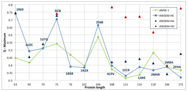
Maximum Q score versus sequence length for “homologs excluded” AWSEM (AWSEM-HE, light blue squares) and AMW-1 (green diamonds) models. Maximum Q scores for “homologs allowed” (AWSEM-HA, dark blue triangles) and “homologs only” (AWSEM-HO, red triangles) are also shown where available.

Figure 5.

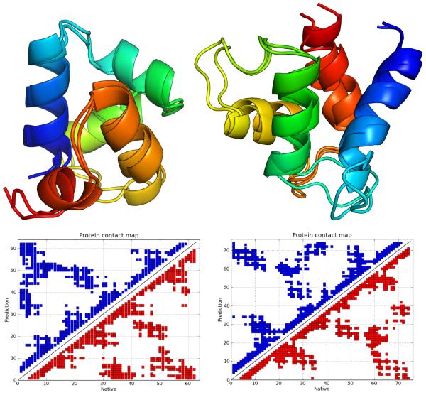
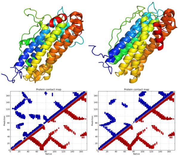
Structural alignments and comparative contact maps of the maximum Q score structures obtained from “homologs excluded” predictions for 1R69 (on the left, Q = 0.74, RMSD 1.6Å ) and 3ICB (on the right, Q = 0.703, RMSD 2.4Å ).

Analyses

To evaluate the predictive capability of our model, we calculated the structural similarity of all snapshots from the 20 trajectories of a given target sequence against the corresponding experimentally determined structure. As specific measures of similarity, both Q and RMSD were used, where Q is an order parameter which compares pairwise distances among residues between two structures, as elaborated below. It varies between 0 and 1, with higher values corresponding to higher similarity between the structures. The form of Q is given in Eq. (4),

$$Q=\frac{2}{(N-2)(N-3)}\sum _{i<j-2}\exp \left[-\frac{{(r_{ij}-r_{ij}^N)}^2}{2{\sigma }_{ij}^2}\right],$$ (4)

where N is the total number of residues, r_{i j} is the instantaneous distance between C_α atoms of residues i and j, $r_{ij}^N$ is the same distance in the experimentally determined structure and σ_{i j} is given as σ_{i j} = (1+|i−j|)^0.15.

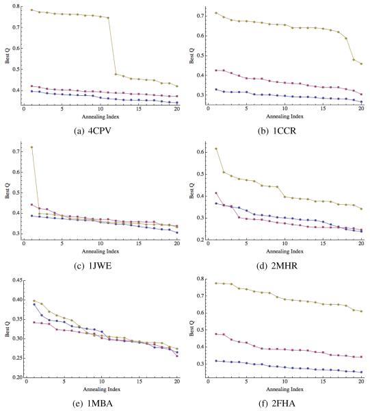
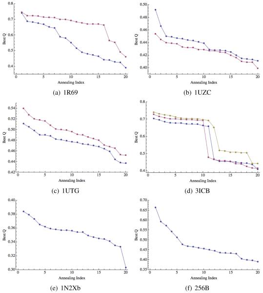
To demonstrate the prediction quality for each of our targets, we have plotted the best Q values from each of the 20 annealing runs, sorting them in descending order (see Figures 2 to 4 and 9). These plots show how stable the predictions are, i.e., what maximum Q values could be expected if fewer simulated annealing runs were performed.

Figure 2.

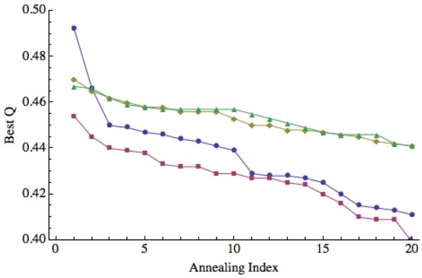
Prediction quality for 1UZC, including and excluding disordered region. For each of the 20 annealing simulations, the maximum Q values obtained are plotted in descending order. Blue circles correspond to “homologs excluded” predictions and red squares to “homologs allowed” predictions when the disordered region is included in the calculation of Q. Green triangles correspond to “homologs excluded” predictions and orange diamonds to “homologs allowed” predictions when the disordered region is excluded from the calculation of Q.

Figure 4.

Prediction quality for 4CPV (a), 1CCR (b), 1JWE (c), 2MHR (d), 1MBA (e), and 2FHA (f). Blue circles correspond to “homologs excluded” predictions, red squares to “homologs allowed” predictions and orange diamonds correspond to “homologs only” predictions.

Figure 9.

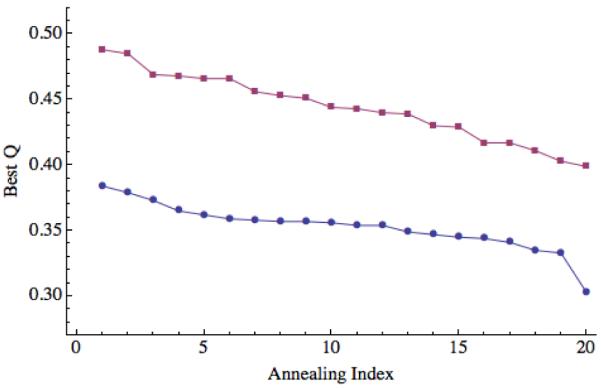
Prediction quality for 1N2X, including and excluding the first 22 residues, a disordered region. For each of the 20 annealing simulations, the maximum Q values obtained are plotted in descending order. Blue circles correspond to the maximum Q values when the disordered region is included and the red squares correspond to the maximum Q value when the disordered region is excluded from the calculation of Q.

We used the CE alignment server³⁸ to align the maximum Q structures with native structures for visual comparison; see Figures 5 to 7.

Figure 7.

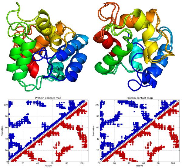
Structural alignments and comparative contact maps of the maximum Q score structures for 4CPV, with the “homologs excluded” prediction on the left (Q = 0.396, RMSD 5.8Å) and the “homologs only” prediction on the right (Q = 0.784, RMSD 1.3Å).

Results

We have summarized our structure prediction results in Figure 1, wherein we have plotted the maximum Q value achieved for a particular target sequence versus its sequence length. The 3 data sets are for the “homologs excluded” (light blue squares), “homologs allowed” (dark blue triangles) and “homologs only” (red triangles) fragment libraries. We have also plotted the AMW-1 results⁶ (green diamonds) for comparison.

The results from both the “homologs excluded” and “homologs allowed” fragment libraries are overall slightly improved compared to the results of the AMW-1 model. The “homologs only” library, which we generated only for sequences with a sufficient number of homologs in our culled database, significantly outperformed the AMW-1, “homologs excluded” and “homologs allowed” models for all target sequences except 1MBA and 3ICB.

Maximum Q values for each of the 20 annealing runs (sorted in descending order) are shown in Figure 3 and Figure 4. These figures show that, in most cases, the predictions are stable, meaning that performing only 5 to 10 annealing runs would have yielded a similar maximum Q value. Two exceptions worth mentioning here are the “homologs only” prediction for 1JWE, and the “homologs excluded” prediction for 1UZC. For the former, the maximum Q value of 0.7 is the only point above Q = 0.4. For the latter, there is a more modest “jump” from Q = 0.45 to Q = 0.47 and 0.49. A close examination of the results for 1UZC indicated that a disordered region on the N-terminal was likely responsible for the erratic results. Figure 2 shows the results when this 11 residue segment was excluded from the calculations of Q. Without this region, the prediction is better on average and significantly more stable.

Figure 3.

Prediction quality for 1R69 (a), 1UZC (b), 1UTG (c), 3ICB (d), 1N2Xb (e), and 256B (f). Blue circles correspond to “homologs excluded” predictions, red squares to “homologs allowed” predictions and orange diamonds correspond to “homologs only” predictions.

Finally, we compared our “homologs only” results with the popular comparative structure prediction package MODELLER^32-34 using the same homologs that were used for the “homologs only” simulations. The results are summarized in Figure 8, where blue squares are the best RMSD values for “homologs only” AWSEM and orange diamonds are the MODELLER results.

Figure 8.

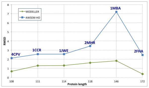
Comparison of MODELLER (green diamonds) and AWSEM (blue squares) prediction quality, showing RMSD in Å to the experimental structure versus sequence length in amino acids.

Discussion

As shown in Figure 1, the predictions made by AWSEM using the “homologs excluded” fragment library are in general improved compared to the AMW-1 results.⁶ Before giving a more comprehensive comparison, we will briefly mention the key differences between AWSEM and AMW-1. The two models share the same backbone, direct contact, protein/water-mediated contact and burial potentials. However, AMW-1 used globally aligned protein sequences to specify associative memory interactions, whereas AWSEM uses short fragments to bias the local conformational search. In addition, AWSEM includes an explicit helical hydrogen bonding potential, and does not use a radius of gyration biasing term. The latter was shown to play an important role in correctly predicting the structure of large, non-spherical proteins.⁷

For 1R69 and 3ICB, maximum Q values of ~ 0.75 and ~ 0.7 are highly significant improvements of ~ 0.3 and ~ 0.15, respectively, compared to the AMW-1 predictions. Figure 5 shows an alignment of the predicted and native structures, and comparative contact maps for 1R69 and 3ICB, which indicate precise prediction of all secondary structure elements as well as good agreement of the global folds. AWSEM predictions of 1BG8, 2MHR and 2FHA were slightly worse than those of AMW-1.

The number of homologs available for each sequence varied from one to twenty (see Table 1). By performing predictions with the “homologs allowed” fragment library, we determined that the effect of including fragments from globally homologous sequences among other fragments from non-homologous sequences on the quality of prediction is small. In fact, the improvement was statistically significant for four proteins, of which only two had a change in the maximum Q value of 0.1 or more. Specifically, the maximum Q values for 1CCR and 2FHA improved by 0.1 (from 0.33 to 0.43) and by 0.16 (from 0.319 to 0.474), respectively. The improvement for 2FHA can be seen in the structural alignment and contact maps in Figure 6. Unlike the “homologs excluded” prediction, wherein only 3 of the 5 helices are well formed, in the “homologs allowed” prediction all helices are formed and 4 of them, with the exception of the small C-terminal helix, have the correct mutual orientation and packing. This is particularly impressive given the size (172 residues) and non-symmetric shape of 2FHA.

Figure 6.

Structural alignments and comparative contact maps of the maximum Q score structures for 2FHA, with the “homologs excluded” prediction on the left (Q = 0.319, RMSD 12.383Å) and the “homologs allowed” prediction on the right (Q = 0.476, RMSD 8.781Å).

For five of the seven targets predicted using the “homologs only” library, AWSEM achieved a maximum Q greater than 0.7. For 2MHR, a maximum Q = 0.62 and minimum RMSD of 3.44Å was obtained. For 1MBA, the maximum Q obtained was 0.4. To evaluate these results, we compared them with structure prediction results obtained using the MODELLER package. This package can do all-atom comparative modeling of proteins using experimentally determined structures, and their sequence alignments with the target sequence by satisfying spatial restraints. MODELLER was able to predict the structure of all larger proteins within 2Å RMSD resolution (Figure 8). Except for 1MBA, the difference in RMSD between the AWSEM prediction and the MODELLER prediction is between 1 and 2 Å . This implies that, despite being a coarse-grained model lacking explicit side chains, AWSEM can be used to make high resolution predictions for sequences that have homologs with experimentally determined structures.

There are several possible contributing factors to AWSEM’s relatively poor prediction of 1MBA. Of all the target sequences, 1MBA has the homologs with the lowest sequence identity, with a maximum of 32.64%. As a result, even though there are 26 homologs in the database with 95% MMSI, the number of fragments assigned per position varied from 0 to 14 with an average value of 3. This inhomogeneity cannot be overcome simply by scaling the strength of the fragment memory term. In such cases it would be useful to introduce a smarter normalization and weighting scheme within the fragment memory potential based on the number of interactions per residue, fragment length and alignment quality. The fragment memory potential could also potentially be improved by optimizing with respect to the fragment length and fragments per position. We did not test these possibilities here. Finally, unlike MODELLER, AWSEM lacks all-atom side chains, which may play an important role in 3 dimensional packing. This type of effect might accumulate and become particularly important for large proteins, such as 1MBA (146 residues). On the other hand, we should also bear in mind that MBA has a heme cofactor which is entirely omitted in our present simulations.

Another important factor to consider when analyzing the quality of prediction results is the presence of disordered and flexible terminal regions (or tails). Because these regions lack a static structure, “errors” in the prediction of these regions will have the effect of artificially lowering and broadening the distribution of Q values and RMSD scores we get. This broadening effect is apparent in Figure 2, where exclusion of the flexible tail from Q calculations of 1UZC collapses the “homologs excluded” and “homologs allowed” results, causing them to both be more similar to each other and making them individually more stable. Similarly, excluding the flexible tail (first 22 residues) from the Q calculations of 1N2X (see Figure 9) systematically increases the maximum we obtain Q in each simulation by 0.1.

Conclusions

Steady progress has been made in the last two decades in addressing the practical aspect of the “Protein Folding Problem”, namely predicting the three-dimensional structures of proteins from their sequence. While early efforts were almost exclusively based on knowledge-based potentials, more recent work uses a mix of physical and bioinformatic approaches. The rapid advances in designing and building specialized computer hardware already allow the use of all-atom explicit solvent simulations to successfully predict structures of some small proteins.³⁹ Nevertheless, given that the average human protein is over 400 residues, and many important and poorly understood biological processes involve complex multi-protein or nucleic acid assemblies, it will be rather difficult to apply atomistic simulations to routinely address these large length- and time-scales processes for some time. Hence, there remains a significant need for the development of coarse-grained, yet preferably accurate protein force fields. Most prior kinetic and mechanistic studies using coarse-grained protein force fields relied on native structure based approaches, which assign favorable interactions to native contacts, giving in concrete terms a folding funnel. While such approaches are physically meaningful, rooted in the energy landscape theory of protein folding, they can underestimate or often completely ignore the role of non-native interactions, cannot be used for proteins without solved structure, and also cannot be directly applied without modification to partially or fully disordered proteins. The above discussion underlines a need for development of a coarse-grained protein force field which is substantially based on known physical interactions, is amenable to Molecular Dynamics simulations and can be used for both de novo protein structure prediction as well as for probing protein folding and dynamics.

AWSEM, which is a successor to the AMH and AMW approaches to protein structure prediction, represents one such force field. It combines a large number of physical interactions, from backbone terms to direct- and water-mediated interactions and hydrogen bonding, with structural biases that are local in sequences, based on the alignments of fragments of nine-residues or less of the target protein to the local segments found in a protein database. The force field was implemented from the ground up in C++, leveraging the LAMMPS molecular dynamics package. It can be used not only for protein structure prediction, but also, for example, to study protein folding kinetics, functional dynamics of the native state, and binding and folding processes. In on-going works, our research groups plan to explore the extensions of AWSEM to simulate disordered proteins and interactions of proteins with membranes and DNA.

In this work, we have shown that the best structures produced by AWSEM in the “blind prediction mode”, where we ensured that no global homologs were included in the local fragments database, were either comparable in quality or improved over the prior AMW efforts in blind prediction. We have also analyzed the consistency of prediction runs. We find that when poorly-defined loops or tails are excluded from the structural comparisons, then there is considerable consistency between different runs for almost all proteins. For some proteins, such as 1R69 and 3ICB, impressive predictions were achieved, with 1.6 Å and 2.4 Å RMSDs to the corresponding native structures. For larger proteins, over 100 residues, the consistency of predictions has some-what improved compared to AMW. For these larger proteins, AWSEM obtains maximal Q values in the range of 0.35 to 0.4. This is often indicative of many native-like structural elements and even a roughly correct overall fold in some cases, but with a number of packing defects among the secondary structural elements. How to take de novo structure prediction of large proteins to the high-resolution levels that are achievable for many smaller proteins is a challenging question, no doubt requiring further efforts in force field development and parameter optimization.

If the goal is not blind protein structure prediction, but instead investigation of protein folding kinetics and protein function, it may be advisable to bias the fragment library with homologs of the target protein, even distant ones. While exploring this possibility, we have shown in this work that even large proteins (on the order of 200 residues) fold to structures that are similar to the corresponding native structures within 1-3 Å RMSD. Hence, by appropriately tuning the fragment library, one may use AWSEM-based coarse-grained modeling of proteins either for de novo structure prediction, or in cases where the structures of distant homologs are known, kinetics and dynamics can be the main aims of the study. As an alternative to using experimentally determined structures for memories, snapshots of highly populated states sampled in atomistic simulations can be used as fragment memories for subsequent AWSEM coarse-grained simulations of the same protein.⁴⁰

Since AWSEM is an open-source package, many groups may choose to contribute to its further development and applications to new areas of research. The comprehensive description of the AWSEM force field, along with all force field parameters, are elaborated in the Supplemental Information, allowing the possibility of reimplementing AWSEM in alternative programming environments.

References

- (1).Service RF. Science. 2008;321:784–786. doi: 10.1126/science.321.5890.784. [DOI] [PubMed] [Google Scholar]
- (2).Fersht A. Structure and Mechanism in Protein Science: A Guide to Enzyme Catalysis and Protein Folding. W. H. Freeman and Co.; New York: 1999. [Google Scholar]
- (3).Pauling L, Corey R, Branson H. Proc. Natl. Acad. Sci. USA. 1951;37:205–211. doi: 10.1073/pnas.37.4.205. [DOI] [PMC free article] [PubMed] [Google Scholar]
- (4).Kauzmann W. Adv. Protein Chem. 1959;14:1–63. doi: 10.1016/s0065-3233(08)60608-7. [DOI] [PubMed] [Google Scholar]
- (5).Wolynes PG, Ulander J, Wolynes PG. J. Am. Chem. Soc. 2003;125:9170–9178. doi: 10.1021/ja034729u. [DOI] [PubMed] [Google Scholar]
- (6).Papoian GA, Ulander J, Eastwood M, Luthey-Schulten Z, Wolynes PG. Proc. Natl. Acad. Sci. USA. 2004;101:3352–3357. doi: 10.1073/pnas.0307851100. [DOI] [PMC free article] [PubMed] [Google Scholar]
- (7).Zong C, Papoian GA, Ulander J, Wolynes PG. J. Am. Chem. Soc. 2006;128:5168–5176. doi: 10.1021/ja058589v. [DOI] [PubMed] [Google Scholar]
- (8).Okeljas V, Zong C, Papoian GA, Wolynes PG. Methods. 2010;52:84–90. doi: 10.1016/j.ymeth.2010.05.006. [DOI] [PMC free article] [PubMed] [Google Scholar]
- (9).Bryngelson JD, Onuchic JN, Socci ND, Wolynes PG. Proteins: Struct., Funct., Genet. 1995;21:167–195. doi: 10.1002/prot.340210302. [DOI] [PubMed] [Google Scholar]
- (10).Wolynes PG. Phil. Trans. R. Soc. A. 2005;363:453–467. doi: 10.1098/rsta.2004.1502. [DOI] [PubMed] [Google Scholar]
- (11).Goldstein R, Luthey-Schulten Z, Wolynes PG. Proc. Natl. Acad. Sci. USA. 1992;89:4918–4922. doi: 10.1073/pnas.89.11.4918. [DOI] [PMC free article] [PubMed] [Google Scholar]
- (12).Goldstein R, Luthey-Schulten Z, Wolynes PG. Proc. Natl. Acad. Sci. USA. 1992;89:9029–9033. doi: 10.1073/pnas.89.19.9029. [DOI] [PMC free article] [PubMed] [Google Scholar]
- (13).Eastwood M, Hardin C, Luthey-Schulten Z, Wolynes P. IBM J. Res. Dev. 2001;45:475–497. [Google Scholar]
- (14).Friedrichs M, Wolynes PG. Science. 1989;246:371–373. doi: 10.1126/science.246.4928.371. [DOI] [PubMed] [Google Scholar]
- (15).Sasai M, Wolynes P. Phys. Rev. Lett. 1990;65:2740–2743. doi: 10.1103/PhysRevLett.65.2740. [DOI] [PubMed] [Google Scholar]
- (16).Friedrichs M, Wolynes PG. Tetrahedron Comput. Methodol. 1990;3:175–190. [Google Scholar]
- (17).Friedrichs M, Goldstein R, Wolynes PG. J. Mol. Biol. 1991;222:1013–1034. doi: 10.1016/0022-2836(91)90591-s. [DOI] [PubMed] [Google Scholar]
- (18).Sasai M, Wolynes P. Phys. Rev. A. 1992;46:7979–7997. doi: 10.1103/physreva.46.7979. [DOI] [PubMed] [Google Scholar]
- (19).Hardin C, Eastwood M, Luthey-Schulten Z, Wolynes PG. Proc. Natl. Acad. Sci. USA. 2000;97:14235–14240. doi: 10.1073/pnas.230432197. [DOI] [PMC free article] [PubMed] [Google Scholar]
- (20).Hardin C, Eastwood M, Prentiss M, Luthey-Schulten Z, Wolynes PG. Proc. Natl. Acad. Sci. USA. 2003;100:1679–1684. doi: 10.1073/pnas.252753899. [DOI] [PMC free article] [PubMed] [Google Scholar]
- (21).Hopfield J. J. Proc. Natl. Acad. Sci. USA. 1984;81:3088–3092. doi: 10.1073/pnas.81.10.3088. [DOI] [PMC free article] [PubMed] [Google Scholar]
- (22).Kuhlman B, Dantas G, Ireton GC, Varani G, Stoddard BL, Baker D. Science. 2003;302:1364–1368. doi: 10.1126/science.1089427. [DOI] [PubMed] [Google Scholar]
- (23).Noid WG, Chu J-W, Ayton GS, Krishna V, Izvekov S, Voth GA, Das A, Andersen HC. J. Chem. Phys. 2008;128:244114. doi: 10.1063/1.2938860. [DOI] [PMC free article] [PubMed] [Google Scholar]
- (24).Savelyev A, Papoian GA. Biophys. J. 2009;96:4044–4052. doi: 10.1016/j.bpj.2009.02.067. [DOI] [PMC free article] [PubMed] [Google Scholar]
- (25).Savelyev A, Papoian GA. J. Phys. Chem. B. 2009;113:7785–7793. doi: 10.1021/jp9005058. [DOI] [PubMed] [Google Scholar]
- (26).Maisuradze GG, Senet P, Czaplewski C, Liwo A, Scheraga HA. J Phys Chem A. 2010;114:4471–4485. doi: 10.1021/jp9117776. [DOI] [PMC free article] [PubMed] [Google Scholar]
- (27).Saven J, Wolynes PG. J. Mol. Biol. 1996;257:199–216. doi: 10.1006/jmbi.1996.0156. [DOI] [PubMed] [Google Scholar]
- (28).Hegler J, Lätzer J, Shehu A, Clementi C, Wolynes PG. Proc. Natl. Acad. Sci. USA. 2009;106:15302–15307. doi: 10.1073/pnas.0907002106. [DOI] [PMC free article] [PubMed] [Google Scholar]
- (29).Plimpton S. J. Comput. Phys. 1995;117:1–19. [Google Scholar]
- (30).Savelyev A, Papoian GA. Proc. Natl. Acad. Sci. USA. 2010;107:20340–20345. doi: 10.1073/pnas.1001163107. [DOI] [PMC free article] [PubMed] [Google Scholar]
- (31).Hyeon C, Morrison G, Pincus DL, Thirumalai D. Proc. Natl. Acad. Sci. USA. 2009;106:20288–20293. doi: 10.1073/pnas.0905764106. [DOI] [PMC free article] [PubMed] [Google Scholar]
- (32).Marti-Renom M, Stuart A, Fiser A, Sánchez R, Melo F, Sali A. Annu. Rev. Biophys. Biomol. Struct. 2000;29:291–325. doi: 10.1146/annurev.biophys.29.1.291. [DOI] [PubMed] [Google Scholar]
- (33).Sali A, Blundell T. J. Mol. Biol. 1993;234:779–815. doi: 10.1006/jmbi.1993.1626. [DOI] [PubMed] [Google Scholar]
- (34).Fiser A, Do R, Sali A. Protein Sci. 2000:1753–1773. doi: 10.1110/ps.9.9.1753. [DOI] [PMC free article] [PubMed] [Google Scholar]
- (35).Berman H, Westbrook J, Feng Z, Gilliland G, Bhat T, Weissig H, Shindyalov I, Bourne P. Nucleic Acids Res. 2000;28:235–242. doi: 10.1093/nar/28.1.235. [DOI] [PMC free article] [PubMed] [Google Scholar]
- (36).Wang G, Dunbrack R. Bioinformatics. 2003;19:1589–1591. doi: 10.1093/bioinformatics/btg224. [DOI] [PubMed] [Google Scholar]
- (37).Altschul SL, Madden T, Schäffer A, Zhang J, Zhang A, Miller W, Lipman D. Nucleic Acids Res. 1997;25:3389–3402. doi: 10.1093/nar/25.17.3389. [DOI] [PMC free article] [PubMed] [Google Scholar]
- (38).Shindyalov I, Bourne P. Protein Eng. 1998;11:739–747. doi: 10.1093/protein/11.9.739. [DOI] [PubMed] [Google Scholar]
- (39).Shaw DE, Maragakis P, Lindorff-Larsen K, Piana S, Dror RO, Eastwood MP, Bank JA, Jumper JM, Salmon JK, Shan Y, Wriggers W. Science. 2010;330:341–346. doi: 10.1126/science.1187409. [DOI] [PubMed] [Google Scholar]
- (40).Kwac K, Wolynes PG. Bull. Korean Chem. Soc. 2008;29:2172–2182. [Google Scholar]
Associated Data
This section collects any data citations, data availability statements, or supplementary materials included in this article.