Associative memory Hamiltonians for structure prediction without homology: Alpha-helical proteins

Abstract

Energy landscape theory is used to obtain optimized energy functions for predicting protein structure, without using homology information. At short sequence separation the energy functions are associative memory Hamiltonians constructed from a database of folding patterns in nonhomologous proteins and at large separations they have the form of simple pair potentials. The lowest energy minima provide reasonably accurate tertiary structures even though no homologous proteins are included in the construction of the Hamiltonian. We also quantify the funnel-like nature of these energy functions by using free energy profiles obtained by the multiple histogram method.

When a protein folds in the test tube, the information contained in its one-dimensional sequence is transformed into the three-dimensional information of its native protein structure. It is not a surprise then that the theory of protein folding has many common themes with more abstract problems of the statistical mechanics of information processing (1). Beyond the analogies at a theoretical level, many approaches to the practical problem of protein structure prediction can profitably be viewed as connectionist schemes for learning the proper sequence–structure associations from the database of known protein structure–sequence pairs. The commonality of viewpoint between folding and machine learning is quite explicit for schemes to predict local secondary structures from sequence that use neural networks (2). Going further, using this philosophy we have developed a series of algorithms for predicting tertiary structure that are based on simulated annealing of “associative memory (AM) Hamiltonians” (3, 4). These models make very active use of statistical mechanical landscape theory and capture the notion of landscapes tunable from those with perfect funnels to nearly random rugged landscapes (5–7). We have shown that these methods work quite well when the database of input structures includes one (or more) homologs. When more than one homolog is present the predicted structures combine good elements of each homolog (8) and indeed give a more accurate structure than any of the inputs. How far can this ability to generalize be pushed? What if no protein with similar overall structure is yet known? Can even small fragments of correct structure in known examples be combined? In this paper we will describe the performance of optimized AM Hamiltonians that do not use homologs in their input. Thus these algorithms provide ab initio predictions of the three-dimensional protein structures. We use the word ab initio not to mean starting from the underlying physiochemical forces alone, as some do, but rather as starting without knowledge of globally similar folds, the less pure but more practical meaning (9).

One crucial idea in understanding protein folding in the laboratory has been that proteins are not randomly chosen systems but are special heteropolymers: their free energy landscape is only minimally frustrated so they fold into unique states rather than having alternate deep traps of wildly different structure. There may be exceptions to this general rule for many biomolecules: prions in nature, the Janus proteins synthesized in the laboratory (10) or, remarkably, some examples in the RNA world. Nevertheless we can use this idea in a practical way by ensuring that any energy function we use is minimally frustrated for those natural proteins that are known to fold to unique (average) low-resolution structures. To do this one must make the idea of minimal frustration a quantitative principle rather than merely a qualitative statement. This quantification involves knowing the phase diagram of the protein model and especially locating the folding and glass transitions (1). One way to do this assumes that in the vicinity of non-native structures the landscape of natural proteins resembles that of a simple random heteropolymer. If so, the minimal frustration principle can be formulated as maximizing the energy gap between native structures and non-native decoys, in units of the energy variance of the misfolded structures. We used this optimization procedure for AM Hamiltonians long ago (4), but it also has been used to find energy functions useful for sequence–structure alignment and to set scaling parameters in energy functions whose form is based on a priori reasoning from detailed molecular physics (11).

Unlike the situation for many machine learning problems formulated in an abstract framework, the structure space for proteins is not uniform and is quite varied: one must discriminate native folds not only from other fully collapsed structures but also from expanded ones with correct secondary structure, collapsed structures with good phase separation between hydrophobic and hydrophilic residues, etc. Different parts of the energy function determine the stability of each of these regions to varying extents. Thus implementing the minimal frustration principle involves an iterative scheme that constrains the statistics of the different classes of decoys and that self-consistently eliminates the deepest non-native traps. We implemented such a scheme for AM Hamiltonians when homologs were included in the database (12). Our goal here is to report on the results of carrying out a similar scheme without using homologs. In addition to describing the energy function and detailed optimization scheme, we present results of simulated annealing using the resulting energy function, limiting ourselves here to a study of all alpha-helical proteins. We also show free energy profiles that quantify how funnel-like or rough are the energy landscapes that result from the optimization scheme.

Materials and Methods

AM, Contact, and Backbone Potentials.

To allow molecular dynamics simulation of the entire folding process, we use a coarse-grained description of the protein. Each amino acid residue is represented by the three atoms, C_α, C_β, and O. The corresponding equations of motion for these atoms involve residue–residue or sequence-dependent interactions in addition to a backbone potential that maintains chain connectivity and correct peptide stereochemistry. Interactions between residues at short to medium range sequence separations are described by AM potentials, and between more distant pairs by a series of piecewise contact potentials whose forms are chosen to roughly mimic the behavior of long-range pair correlations for C_βs. The AM potential is based on correlations between a target's sequence and the sequence-structure patterns in a set μ of memory proteins. The pairs in the target and in the memory are first associated by using a sequence–structure threading algorithm (4, 8), and in the present ab initio folding study, the memory proteins contain no protein homologous to the targets (see Appendix). Table 1 lists the highest Q memory protein for each target. Thus only fragmentary, local in sequence patterns are expected to be found by the threading procedure. The energy parameters γ encode similarity between residue pairs i and j in the target and the aligned pairs i′ and j′ in the memory proteins. We use a simplified, four-letter code {P_i} to represent the 20 naturally occurring amino acids. The AM potential encoding these sequence–structure patterns is given by

where the structural similarity is measured by Gaussian functions Θ. The parameters {γ} are learned by the optimization procedure. Between nonadjacent residues the r_ij distances are taken only between the C_α and C_β atoms on each residue. This gives rise to four interactions per residue pair. Different γ values are used for the two proximity classes: short j − i < 5 and medium range 5 ≤ j − i ≤ 12. The specific amino acids in each category are hydrophilic (Ala, Gly, Pro, Ser, Thr), hydrophobic (Cys, Ile, Leu, Met, Phe, Trp, Tyr, Val), acidic (Asn, Asp, Gln, Glu), and basic (Arg, His, Lys). Interactions between residue pairs distant in sequence (|i − j| ≥ 13) are described by pair potentials between pairs of C_β atoms V_long(P_i,P_j,r_ij) = Σ_k=1³ c_k(N)γ_k(P_i,P_j)U(r_ij, r_k), which are approximated by three smoothed square wells covering the regions: 4.5 < r_ij < 8.0, 8.0 < r_ij < 10, 10 < r_ij < 15 (units of Å). The precise form of U(r_ij,r_k) is

where σ controls the sharpness of the potential boundaries, and r_k^min,max are the endpoints of the intervals. The contact potential includes an additional scaling, c_k(N) = 1/(Na_k + b_k), to account for the variation in the number of contacts over the three contact wells. C(N) is found from fitting the number of contacts in each of the regions as a function of the sequence length of the target proteins, and the parameters are given in Table 2.

Table 1.

The Q score and name of the most homologous protein used in the memory set for each training protein

Training protein	Best memory	Q
1r69	2a0b	0.29
1utg	2a0b	0.33
3icb	1nsg	0.33
256B(a)	1au1(a)	0.31
4cpv	1avs(b)	0.29
1ccr	1lki	0.22
2mhr	1rcb	0.27
1mba	1col(a)	0.24
2fha	1vin	0.18
1rgp	1axd	0.20

Table 2.

Backbone potential parameters

λχ	λφψ	λex	λharm	σ	a1, b1	a2, b2	a3, b3
40.0	2.0	20.0	30.0	7 Å−1	1.0	0.0065,0.87	0.0419,0.13

λ_χ, λ_{φψ, λex}, and λ_harm are in units of the AM interaction energy, ɛ. 

The backbone potential, described in detail elsewhere (13, 14), has been updated to include a periodic torsion potential (V_ΦΨ) that provides a better fit to the backbone torsion angles observed in a recent Ramachandran map for nonglycine residues in well-resolved x-ray structures (15). The total potential used in the molecular dynamics simulations is

where V_χ is a chirality potential that biases L-amino acid chirality, V_ex are the excluded volume potentials applied to nonbonded carbon and oxygen atoms that approach within 3.5 Å for (j − i) < 5, and 4.5 Å for (j − i) ≥ 5. V_harm is the sum of three quadratic potentials that are used along with a series of shake (16) constraints to provide backbone rigidity, maintain the planarity of the peptide bond, and maintain the appropriate bond angles. The sequence-dependent potentials, V_AM and V_contact, are simultaneously optimized as described below. The energy parameters γ have been scaled so that the average value of the native state energy per residue per interaction over the training set is 1. The weights of the backbone terms, listed in Table 2, have been empirically chosen.

Constrained Self-Consistent Optimization.

The simplest statistical mechanical treatment of the phase diagram depends on only a few average properties of native structures and globules. The glass transition temperature is given by the energetic variance of the misfolded ensemble T_g ≃ The collapse temperature depends on the mean energy of the globule states, T_c ≃ The folding temperature T_f is given by the ratios of the difference in energy between the native state and the globules and the entropy, T_f ≃ δE/S_c. More elaborate polymer theoretical estimates of compact globules suggest this is a good approximation (17). We find these collapsed structures do have some nativelike components. The structures or conformations in the molten globule ensemble have an average Q-value of 0.2 and a radius of gyration R_g of 1.2. The unconstrained maximization of is equivalent to maximizing the ratio

In the AM Hamiltonians the potentials are a sum of terms ξ_i, each representing a basic form of interaction. In the present study, the ξ_is depend on amino acid class and the proximity of two amino acids in the sequence, as described above. If the interactions are weighted by linear parameters γ_i, the energy gap and variance (and the corresponding temperatures) can be expressed simply as δE = Aγ and ΔE² = γBγ. A and γ are vectors of dimensionality equal to the number of interaction types, and B is a matrix given by

These averages depend on the frequencies at which any given interaction occurs in the molten globule and native configurations. Maximizing the energy ratio amounts to varying the interaction weights γ_i and leads to an optimization problem that can be solved by straightforward linear algebra, γ = B⁻¹ A up to a scalar multiple.

The mean energy of the molten globule distribution (and the corresponding collapse temperature) is a linear function of the interaction weights, 〈E〉_mg = A′γ.

For off-lattice models, unlike many lattice model studies of sequence design and folding kinetics, which often concentrate on fully collapsed structures alone, efficient folding via molecular dynamics simulation requires a more complete statistical mechanical treatment of the phase diagram. These better approximations must account for the existence of partially ordered ensembles of states, with varying degrees of collapse and secondary structure formation (4, 12). So that such states not become competitive with the native state energy, the contribution to the mean energy of the globules from interactions in each proximity class are constrained. In models with interactions of different ranges there also can be different glass transition temperatures associated with structures on different length scales. This behavior is predicted by the generalized random energy model of Derrida (18), which has been used for random heteropolymers with contact potentials (17). It is necessary to constrain the variances, as well as the means, of subensembles, otherwise too large interactions in the short sequence range could lead to the dynamical freezing of short-range interactions, for example, at a temperature that is high relative to the T_g for fixing structures involving the more distant in sequence interactions (19). The mean energy and variance of the molten globule distribution expressed in terms of contributions from the short-, intermediate-, and long-range interactions are fixed by imposing linear constraints in the following optimization functional

where the first two terms in the sums correspond to the secondary and supersecondary interactions, λ_k are the Lagrangian multipliers, and c_k the constraint values. Maximizing this functional is equivalent to maximizing the folding temperature (energy gap) while fixing the collapse and glass transition temperatures of the subensembles. In writing the functional we have ignored correlations between the various interaction classes. Indeed these correlations are so small that they are hard to statistically determine by sampling. The constraints are chosen so that the energy of any molten globule configuration is evenly distributed among the length scales (20). Because the globules have flickering, native-like elements the glass transition temperature T_g is estimated from the variance B′, which contains only the non-native part of the energy of any molten globule configuration. Projecting out native-like contacts is consistent with the assumptions of the random energy model estimate of T_g. Constrained optimization leads to the simple variational equation

where 〈 〉 indicates an average over a set of training proteins. The ensemble of compact misfolded structures for each training protein is generated initially from translations of the training sequences along a database of unrelated structures. Subsequent iterations are generated by molecular dynamics. Because the misfolded structures are partially ordered and have a tendency to satisfy any especially large interaction energy term, the variational equation is solved iteratively to obtain the interactions weights γ_(n). In this self-consistent optimization the low-energy misfolded structures are generated through molecular dynamics simulations by using the γ_(n−1) values from the previous round. The ensembles are generated in constant temperature simulations and the structures are censored to have Q < 0.4. Each round of optimization combines the interaction parameters from previous optimization by a simple average, γ′_n = ɛγ_n−1 + (1 − ɛ)γ_n. This is analogous to conjugate gradient optimization.

At each step n in the constrained self-consistent optimization, the energy gaps and variances of the molten globule states obtained in constant temperature molecular dynamics simulations with the γ_n−1 iterate energy parameters were evaluated. The optimized interaction weights γ are the solutions of the matrix linear algebra equation (12) for the training set and the current set of misfolded states. The AM Hamiltonian with two proximity classes has 512 interaction weights, and the contact potential with three proximity classes has an additional 30. For a given set of training proteins and a given misfolded ensemble, some of these interactions may be sampled only rarely due to practical limitations on the size of the training set and the set of misfolded states. To avoid attaching an erroneously large weight to such noisy interactions, we have filtered the modes of the B′ matrix with very small variance:

Here M is the matrix of eigenvectors of the unfiltered B′ matrix and (λ*)⁻¹ is the diagonal matrix obtained from the diagonal matrix of eignvalues by zeroing out eigenvalues below a cut-off. By setting small eigenvalues equal to zero, we ignore these modes.

Results

The interaction weights γ were optimized by using a set of well-resolved Protein Databank structures from the class of alpha-helical proteins. Ten training proteins were chosen from the most populated fold architectures (topologies) in the Cath (21) database: nonbundle [1r69(434repressor), 1utg(uteroglobin), 3icb(recoverin), 4cpv(recoverin), 1ccr(arc repressor), 1mba(globin), 1rgp(G-protein, GTPase Activation domain)] and bundle [2mhr(four-helix bundle), 256ba(four-helix bundle), 2fha(granulocyte colony-stimulating factor)]. The 10 training proteins were aligned to a set of 36 alpha-helical proteins (see Appendix) by using the threading algorithm of Koretke et al (8). Individual memory sets were modified so that each one contained no proteins homologous to the training protein used. The alignments of the training proteins to the corresponding sets of memory proteins constitute the AM Hamiltonian.

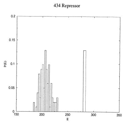
The gaps and variances generated with the last round of iteration are shown in Fig. 1. Consistent with the imposed constraints, the energy gap between the folded state and the mean of the molten globule distribution is roughly equally divided between the short-range and long-range interactions.

Figure 1.

Distribution of conformational energies for the 434 repressor. The figure shows the energies of the misfolded ensemble of states as well as that of the native state. The misfolded conformations were generated in a constant temperature molecular dynamics simulation at a reduced temperature of 1.2. Energies were evaluated by using the final interaction weights obtained from the self-consistent optimization procedure.

Structure Prediction Without Homologs via Molecular Dynamics

Starting from extended configurations with randomized φψ angles, the 10 training set proteins and three proteins that were not part of the training set were annealed by molecular dynamics using the energy parameters corresponding to Fig. 1. Using the standard annealing protocol, each run uses approximately 6 h on a SGI Origin 200 workstation. The results seem to be well equilibrated, so it is possible shorter runs would do as well. We measure the progress of the molecular dynamics trajectories by means of two order parameters, Q and Q_cut. Q is the fraction of all native C_α pair distances, and Q_cut is the same fraction, counting only pairs within some cut-off distance:

Here r_ij refers to C_α distances, and we have chosen r_c = 8.0 Å. The advantage of Q_cut is in its similarity to typical contact order parameters, such as have been used in lattice studies. The off-lattice Q, on the other hand, includes pairs that are separated by large distances and is sensitive to domain rotations and other distortions.

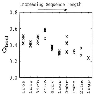
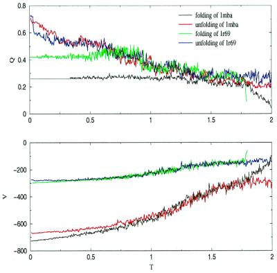
The Q of the best structure in each of the runs performed for all 10 training proteins is given in Fig. 2. The data in the figure indicate that simulated annealing using the energy function is more successful on shorter proteins than it is on longer ones. Fig. 3 presents sample folding and unfolding trajectories for 434 repressor, of length 63, and myoglobin, which has length 146. The folding trajectory of myoglobin is typical of the longer training proteins, in that collapse to nearly the final value of Q occurs at a relatively high temperature. Moreover, the size of the fluctuations in Q is somewhat smaller than in the case of the repressor. Both of these observations suggest that the collapse characteristics of the energy function are not yet optimum for longer proteins. Even so comparison of the folding and unfolding trajectories shows that the potential yields more native-like structures with energies comparable to those of the best structures in the folding run. Although it has lower overall quality, the Q_best structure still has a Q of over 0.4 for up to half of the molecule.

Figure 2.

Q_best values obtained from the simulated annealing runs of the 10 training proteins. The proteins are ordered by sequence length. A total of 2–5 runs were performed for member of the training set and the best Q encountered in the run is plotted as Q_best.

Figure 3.

Folding and unfolding trajectories for myoglobin (1mba) and 434 repressor (1r69). (Upper) Q as a function of temperature. (Lower) The potential energy as a function of temperature.

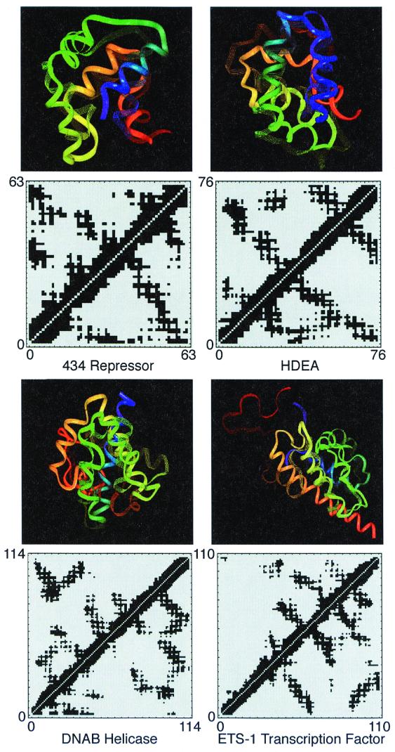
For the test set we chose three alpha-helical targets from the CASP3 structure prediction experiment (22), which were rated as moderately difficult: 1bg8(a), 1jwe, and 1bqv. Again, no homologous proteins were used in the memory set. Furthermore, these proteins are not homologs of any of those used in training. As shown in Table 3, our method gives substantially correct structures for these proteins. The superpositions of predicted and native structures in Fig. 4 indicate that the correct topology has been achieved over the majority of the protein in all cases. The Q_best structures appearing in Table 3 are typically sampled near the folding temperature and further annealing degrades the overall structure as shown in the folding trajectories in Fig. 3. The precise structures observed at low temperatures typically have energies lower than that of the x-ray structure.

Table 3.

Summary of results from simulated annealing of test set proteins

Protein	N	Qbest	rmsdbest	Qf	Nf	rmsdf
1bqv	110	0.28	13.2	0.43	70	5.08
1jwe	114	0.28	11.9	0.36	60	7.4
1bg8(a)	76	0.40	8.87	0.44	65	5.3

All simulations began from a random coil configuration. Q_best is the structure with the best overall Q, rmsd_best is the rms deviation of that structure. Q_f, N_f and rmsd_f refer to superpositions of fragments of the best Q structure onto the corresponding fragment of the x-ray structure. 

Figure 4.

Structural alignments of Q_best structures from simulated annealing of one training set protein (434 repressor) and the three test set proteins to their x-ray structures. Native structures are shown as lines, and the predicted structures as solid ribbons.

At any given temperature the structure of the energy landscape may be explored more quantitatively by examining the total free-energy and energy as a function of Q_cut. Using a multiple-histogram sampling technique (23), we computed the free energy profiles for our optimized model. For comparison we also calculated the free energy surface for a Go-like model with the same backbone, which stabilizes only native contacts (24). The Go model possesses a nearly ideal, funneled landscape (14). The results of this analysis at a temperature near the folding temperature are shown in Fig. 5. In both cases, the total energy is funneled towards the native state, Q_cut = 1. As expected, the Go model is smoothly funneled over the entire range. The energy function optimized for structure prediction yields a more caldera-like landscape. For the training protein 1r69 the landscape is funneled only to about Q_cut = 0.6, after which the energy profile levels off. For 1bg8(a), the deviation from a perfect funnel is more dramatic, with the energy actually increasing somewhat as higher Q states are sampled.

Figure 5.

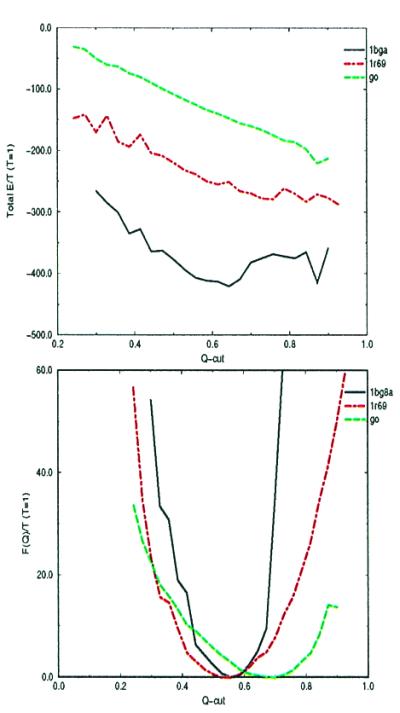
Energy and free energy as a function of Q_cut for the training protein 434 repressor, the test protein HDEA, and a Go model.

Conclusion

The results of this paper show that the present self-consistent optimized AM Hamiltonian allows the ab initio structure prediction of small alpha-helical proteins via molecular dynamics with simulated annealing. Preliminary investigation of a similar treatment for α/β and all β proteins already yields results of similar quality. The ability to predict correct overall structures without using homology information was achieved by introducing a finer division of amino acid classes beyond just simple hydrophobicity as well as constraints to control the energetic balance between short-, intermediate-, and long-range interactions. Degradation in the quality of prediction by simulated annealing with increasing sequence length might be addressed by simply splitting the training set, and separately optimizing for longer proteins. This may reflect an important role of nonadditive forces in the collapse. We see that the AM Hamiltonian framework provides an approach that allows the harmonious marriage of threading and ab initio strategies for protein structure prediction.

Abbreviation

AM

associative memory

Appendix

The 10 alpha-helical proteins varied in length from 63 to 100 and 83 amino acids: 1r69, 1utg, 3cib, 256ba, 4cpv, 1ccr, 2mhr, 1mba, 2fha, 1rgp. They were selected to represent the various classes of well-resolved x-ray structures appearing in the pdb select 95 (25). After removing structures determined by nmr, those with resolution greater than 2.0 Å and those with length greater than 200, pairwise alignments of the remaining proteins were conducted, and the list was iteratively processed to eliminate any protein with a Q to any other protein in the list greater than 0.5. This resulted in a list of 38 proteins from which the memory proteins for the AM Hamiltonian potentials were selected. The selection process eliminated any memory protein with structural overlap greater than Q > 0.4 to any of the training proteins. The 38 memory proteins were: 1a17, 1a28a, 1aa7b, 1aep, 1ah7, 1ail, 1ak0, 1au1a, 1avsb, 1axda, 1b4fh, 1baj, 1beo, 1bgf, 1bjaa, 1bl0a, 1c3d, 1cf7, 1cola, 1e2aa, 1hiws, 1hula, 1huw, 1jhga, 1kxu, 1lbd, 1lis, 1lki, 1nsgb, 1pbv, 1rcb, 1szt, 1tx4a, 1vin, 256ba, 2a0b, 2abk, 5icb.

References

- 1.Wolynes P G. In: Carges Lectures 1990 in Biologically Inspired Physics. Peliti L, editor. New York: Plenum; 1991. pp. 15–37. [Google Scholar]
- 2.Bohr H, Brunak S, Brunak S. Protein Folds: A Distance-Based Approach. London: CRC Press; 1995. [Google Scholar]
- 3.Friedrichs M S, Wolynes P G. Science. 1989;246:371–373. doi: 10.1126/science.246.4928.371. [DOI] [PubMed] [Google Scholar]
- 4.Goldstein R A, Luthey-Schulten Z A, Wolynes P G. Proc Natl Acad Sci USA. 1992;89:4918–4922. doi: 10.1073/pnas.89.11.4918. [DOI] [PMC free article] [PubMed] [Google Scholar]
- 5.Sasai M, Wolynes P G. Phys Rev Lett. 1990;65:2740–2743. doi: 10.1103/PhysRevLett.65.2740. [DOI] [PubMed] [Google Scholar]
- 6.Leopold P E, Montal M, Onuchic J N. Proc Natl Acad Sci USA. 1992;89:8721–8725. doi: 10.1073/pnas.89.18.8721. [DOI] [PMC free article] [PubMed] [Google Scholar]
- 7.Onuchic J N, Luthey-Schulten Z, Wolynes P G. Annu Rev Phys Chem. 1997;48:539–594. doi: 10.1146/annurev.physchem.48.1.545. [DOI] [PubMed] [Google Scholar]
- 8.Koretke K K, Luthey-Schulten Z, Wolynes P G. Protein Sci. 1996;5:1043–1059. doi: 10.1002/pro.5560050607. [DOI] [PMC free article] [PubMed] [Google Scholar]
- 9.Simmons K T, Bonneau R, Ruginski I, Baker D. Protein Struct Funct Genet. Suppl. 1999;3:171–176. [Google Scholar]
- 10.Dalal S, Balasubramanian S, Regan L. Folding Des. 1997;2:71–79. doi: 10.1016/s1359-0278(97)00036-9. [DOI] [PubMed] [Google Scholar]
- 11.Jooyoung Lee A L, Ripolli D R, Pillardy J, Scheraga H A. Proteins Struct Funct Genet. Suppl. 1999;3:149–170. [Google Scholar]
- 12.Koretke K K, Luthey-Schulten Z, Wolynes P G. Proc Natl Acad Sci USA. 1998;95:2932–2937. doi: 10.1073/pnas.95.6.2932. [DOI] [PMC free article] [PubMed] [Google Scholar]
- 13.Friedrichs M S, Goldstein R A, Wolynes P G. J Mol Biol. 1991;222:1013–1034. doi: 10.1016/0022-2836(91)90591-s. [DOI] [PubMed] [Google Scholar]
- 14.Hardin C, Luthey-Schulten Z, Wolynes P G. Proteins Struct Funct Genet. 1999;34:281–294. [PubMed] [Google Scholar]
- 15.Karplus P A. Protein Sci. 1996;5:1406–1420. doi: 10.1002/pro.5560050719. [DOI] [PMC free article] [PubMed] [Google Scholar]
- 16.Ryckaert J, Ciccotti G, Berendsen H. J Comput Phys. 1977;23:327–341. [Google Scholar]
- 17.Plotkin S S, Wang J, Wolynes P G. Phys Rev E. 1996;53:6271–6296. doi: 10.1103/physreve.53.6271. [DOI] [PubMed] [Google Scholar]
- 18.Derrida B. J Phys Lett. 1985;46:L401–L407. [Google Scholar]
- 19.Plotkin S S, Wang J, Wolynes P G. J Chem Phys. 1997;106:2932–2948. [Google Scholar]
- 20.Saven J G, Wolynes P G. J Mol Biol. 1996;257:199–216. doi: 10.1006/jmbi.1996.0156. [DOI] [PubMed] [Google Scholar]
- 21.Orengo C A, Michie A D, Jones S, Jones D T, Swindells M B, Thornton J M. Structure (London) 1997;5:1093–1108. doi: 10.1016/s0969-2126(97)00260-8. [DOI] [PubMed] [Google Scholar]
- 22.Orengo C A, Bray J E, Hubbard T, Loconte L, Sillitoe L. Proteins Struct Funct Genet. Suppl. 1999;3:149–170. doi: 10.1002/(sici)1097-0134(1999)37:3+<149::aid-prot20>3.3.co;2-8. [DOI] [PubMed] [Google Scholar]
- 23.Ferrenberg A, Swendsen R. Phys Rev Lett. 1989;63:1195–1198. doi: 10.1103/PhysRevLett.63.1195. [DOI] [PubMed] [Google Scholar]
- 24.Taketomi H, Ueda Y, Go N. Int J Pept Protein Res. 1975;7:445–459. [PubMed] [Google Scholar]
- 25.Hobohm U, Scharf M, Schneider R, Sander C. Protein Sci. 1992;1:409–417. doi: 10.1002/pro.5560010313. [DOI] [PMC free article] [PubMed] [Google Scholar]