Point process modelling of the Afghan War Diary

Abstract

Modern conflicts are characterized by an ever increasing use of information and sensing technology, resulting in vast amounts of high resolution data. Modelling and prediction of conflict, however, remain challenging tasks due to the heterogeneous and dynamic nature of the data typically available. Here we propose the use of dynamic spatiotemporal modelling tools for the identification of complex underlying processes in conflict, such as diffusion, relocation, heterogeneous escalation, and volatility. Using ideas from statistics, signal processing, and ecology, we provide a predictive framework able to assimilate data and give confidence estimates on the predictions. We demonstrate our methods on the WikiLeaks Afghan War Diary. Our results show that the approach allows deeper insights into conflict dynamics and allows a strikingly statistically accurate forward prediction of armed opposition group activity in 2010, based solely on data from previous years.

The last decade has witnessed a tremendous increase in the availability of data relating to conflicts. For example, the collection of media reports in the ‘Armed Conflict Location and Event Dataset’ (1) provides a small scale but highly curated record of conflict events. More prominently, the release of confidential documents by the WikiLeaks whistleblower website in July 2010 has provided for the first time a large scale (but uncurated) description of the current Afghan conflict. However, most analyses of these and similar data sources do not go beyond visualization and descriptive statistical methods (2–5), for good reasons: first, conflict data is highly heterogeneous and often poorly annotated. For example, the WikiLeaks Afghan War Diary (AWD) data used in this study (Dataset S1) consists of event entries as diverse as elaborate preplanned military activity and spontaneous stop-and-search events. Any plausible attempt to model this data will need to be statistical in nature in order to handle the high levels of noise. Second, it is very difficult to define simple mechanisms that would allow the bottom-up construction of a plausible model.

Here, we develop statistical dynamical modelling methodologies to provide a predictive framework that may be used in policy making. We show that the temporal and spatial dependencies (6, 7) as well as diffusion and advection effects (8, 9) inherent in conflict data make it suitable for the use of a broad class of models, widely employed in ecology and epidemiology, in order to describe the dynamics of disaggregated data. We then develop tools based on ideas from point process statistics (10) to constrain the models. The approach enables us to leverage powerful techniques from point process filtering theory and spatiotemporal statistics (11–14) to carry out inference of the underlying system’s dynamics and to predict the future behavior of the system.

We test the performance of our methods on the AWD, a WikiLeaks release which contains over 75,000 military logs by the USA military, describing events which occurred between the beginning of 2004 and the end of 2009 and providing a high temporal and spatial resolution description of the Afghan war in that period. We show that our approach allows deeper insights in the conflict dynamics than simple descriptive methods by providing a spatially resolved map of the growth and volatility of the conflict. Most remarkably, we show that a model trained on the AWD can predict with surprising statistical accuracy the progression of the conflict in 2010; i.e., a year after the end of the AWD data. We conclude the paper by discussing the importance and potential of statistical modelling of conflict data, as well as offering some consideration as to its wide applicability.

Statistical Methods

Spatial Point Processes and the Stochastic Integro-Difference Equation (SIDE).

Conflict data typically consists of a set of incidents labeled through spatiotemporal coordinates which, when visualized as event markers, are highly spatiotemporally correlated, generally clustered and representative of some underlying structure. In this regard, these data sets are very similar to others encountered in a variety of fields, such as epidemiology (15) and agricultural sciences (16). Poisson point processes provide a convenient and frequently used mathematical framework to model event-based data; in this framework, the probability of observing a certain number of events within a region of interest is given by a Poisson distribution whose mean is the integral over of an intensity function λ(s), . In order to accommodate phenomena such as event clustering, the intensity itself is often modeled as a random function, giving rise to doubly stochastic or Cox processes. A popular class of Cox processes, which will also be considered here, is the log-Gaussian Cox process (LGCP) where the logarithm of the event intensity is assumed to be a Gaussian process (GP). We recall that a GP is wholly defined by (i) a mean function μ(s) describing a global trend and (ii) a covariance function k(s,r) indicating how the field at distinct points in space (s and r) covary (17).

Because conflict data is often logged in a discrete-time format (e.g., the day of an event as opposed to the precise time), we will consider a discrete-time series of continuous-space LGCPs. Formally, let , denote a discrete-time index set and {z_k(s)}, , a set of temporally correlated spatial GPs, each with mean μ_k(s) and covariance function 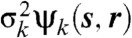. For each k, we then define the point process intensity function as λ_k(s) = exp(z_k(s)). Frequently, the mean function of z_k(s), , can be related to explanatory variables, such as population density, which help to reduce prediction uncertainty. We hence let d(s) be a vector of spatially referenced covariates and b^T the corresponding regression parameters; the LGCP at time k then has intensity λ_k(s) = exp(b^Td(s) + z_k(s)).

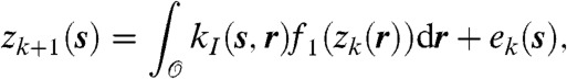
Naturally, the key question is how to specify the temporal dynamics of the intensity functions through z_k(s); we need a sufficiently flexible modelling approach to incorporate the complexity of conflict dynamics. One such representation is the stochastic integro-difference equation (SIDE), a model originally introduced in ecology (18) which has rapidly gained popularity in spatiotemporal statistics (19). The SIDE relates the spatiotemporal dependent variable z_k(s) to z_k+1(s) through the following integral equation

[1]

where k_I(s,r) is the mixing kernel in the integral and e_k(s) is an added disturbance, modeled as a Gaussian field with mean μ_Q(s) and covariance function k_Q(s,r), 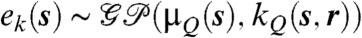, and is the spatial domain under investigation. The nonlinear mapping f₁(·) distorts the field in the sedentary stage; in this work we will employ the identity map f₁(z_k(r)) = z_k(r), an assumption usually adopted in the absence of a priori knowledge (20). The SIDE is, in its original form, a very flexible modelling tool, capable of representing a number of dynamic effects such as diffusion and dispersal (or both simultaneously) even under considerably restrictive conditions (19). Although the AWD will suggest the use of only a special case of SIDE, the two-pronged methodological approach we present here to estimate unknown components is in principle applicable to the more general case.

Nonparametric Analysis.

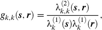
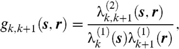
We start by studying the correlation between the conflict events within the same and across subsequent time frames. We are interested in the probabilities of finding a conflict event at r given that an event has occurred at s within the same time frame k or at the previous time frame k - 1. In point process statistics these are quantified through the pair auto-correlation function (PACF) g_k,k(s,r), and what we term the pair cross-correlation function (PCCF) g_k,k+1(s,r) defined as

[2]

[3]

where and are real and positive and denotes the expectation operator.

The PACF may be used to determine qualitative characteristics of the conflict; for instance if g_k,k(s,r) = 1, then no spatial pattern can be extracted from the data; g_k,k(s,r) > 1 and g_k,k(s,r) < 1 can be used to indicate conflict aggregation and repulsion respectively. The PACF can also be used as a preprocessing tool for dimensionality reduction. Direct use of the PACF and PCCF for nonparametric field estimation is also possible (SI Text) but our preliminary investigation showed that this is only a reliable proposition for homogeneous datasets with a very large number of events (SI Text).

Dimensionality Reduction and Bayesian Inference.

In order to develop an inferential approach for SIDE driven LGCPs, we adopt a basis function representation of the spatiotemporal field, which we will then truncate at a level which enables sufficient accuracy (21). This representation, frequently employed in spatiotemporal modelling [e.g., process convolution models (22, 23)], in turn facilitates the implementation of computationally efficient inference algorithms.

The choice of basis functions is a problem that deserves attention; as far as we are aware, there are no standard solutions for LGCPs. We propose here a general approach to selecting basis functions based on the nonparametric estimation of the PACF. Specifically, we capitalize on (i) a fundamental lemma of LGCPs

[4]

which states that the log PACF is proportional to the field auto-correlation function and (ii) the auto-correlation theorem (24) which states that the Fourier transform of the auto-correlation function is the spectrum of the signal. Hence, a relationship between the frequency content of the point process and the PACF is found, which in turn may be used to select a set of sufficiently representative basis functions, much on the lines of refs. 21 and 25. We then obtain a decomposition of the kernel, the mean disturbance and the field as

[5]

[6]

[7]

[8]

where is the vector of basis functions, and are weights which reconstruct the spatiotemporal field and the disturbance mean respectively and where and reconstruct the kernel covariance function and the disturbance covariance function respectively.

It can be shown (SI Text) that under this decomposition, the SIDE of Eq. 1 can be represented in the compact form

[9]

where and is a Gaussian colored noise term with mean and covariance cov[w_k] = Σ_Q. Eq. 9 is a standard linear dynamical system where both the states and the unknown parameters need to be estimated from the data where we define each y_k to be the set of coordinates of the logged events at the kth time point.

For inference, we make use of the likelihood function

[10]

and approximate each λ_k(s) using the same basis representation:

[11]

We proceed with a computationally efficient variational Bayes (VB) method by approximating the full posterior distribution

[12]

where are the variational marginals (26, 27).

The variational marginals are able to reveal important properties of the conflict progression; is used to reconstruct the spatiotemporal field at every time point, ϑ reveals the spatially varying escalation in conflict, Σ_I the extent of any spatial dynamics, if any, and Σ_Q the volatility of the conflict which can either be localized or dependent on events happening at remote geographical locations. The number of unknown parameters in the reduced model scales as , where n is the number of basis functions retained. However, as we will see later, nonparametric data analysis can suggest further simplifications which can considerably lower the complexity of the model.

The Afghan War Diary

On July 25 , 2010, WikiLeaks publicly made available a compendium of US military war logs in Afghanistan dating between 2004 and 2009. The so-called Afghan War Diary contains a detailed insider’s description of the military machinery of the world’s largest power; it consists of roughly 77,000 logs and entries detail the time and position of an event, which could be anything from a stop-and-search episode to a gunfight. The dataset is considered a reliable description of the Afghan war and systematic verification efforts carried out by several organizations such as the New York Times* have found little reason to dispute its authenticity. SI Text reports some of our own tests which show significant correlations between the logged event rate in the AWD and that in other datasets. In what follows we adopt the spatiotemporal point process approach to infer a model from the data in the AWD and use it to analyze the heterogeneous growth (through ϑ) and volatility (through Σ_Q) of the conflict in Afghanistan and also to predict violence of armed opposition groups in 2010, a year after the end of the WikiLeaks dataset.

We start with a nonparametric analysis (SI Text) of the data by splitting the data into weekly intervals (Δ_t = 1 week) and looking at the temporally averaged PACF and PCCF fitted to Gaussian radial basis functions. It is found that, on average, the log PACF is nearly identical to the log PCCF and that a nonparametric estimate of a homogeneous kernel k_I(||s - r||), computed with the direct inverse filter, is very narrow in relation to the extent of the spatial correlations in the field (SI Text). This observation suggests that k_I(·) in the SIDE may be safely approximated to γ(s)δ(s - r), corresponding to negligible spatial interactions across adjacent time frames. Note that if e_k(s) is restricted to be homogeneous and γ(s) = γ, the spatiotemporal covariance function is separable, a common assumption in several fields such as epidemiology (15). However, given the data characteristics, we chose to maintain the spatial heterogeneity in e_k(s). We also set γ(s) = 1 as we found no evidence of mean reversion both at a national and a provincial level; additionally, we found that a spatially dependent γ(s) did not contribute to increased prediction accuracy.

The resulting formulation is validated by studying the temporal dynamics of the AWD (Fig. 1A). A quantitative analysis reveals that the fractional increments of the event incidence nationwide are normally distributed (with a one-tailed Shapiro Wilk’s test and a Levene’s test with α = 0.1, n = 312 w. See also Fig. 1 B and C)^†. This statistic characterizes systems following a geometric Brownian motion given by

[13]

where the increment dW(s,t) is a Gaussian process with zero mean and covariance function k_Q(s,r)dt and is a spatially varying percentage drift. Applying Ito’s Lemma (28) to ln λ(s,t) and noting that the continuous-time intensity ln λ(s,t) = b^Td(s) + z(s,t), we obtain the following form for z(s,t):

[14]

where is a heterogeneous temporally independent spatial growth rate and σ(s)² is the variance field. Applying an explicit Euler discretization scheme to Eq. 14, one obtains the model z_k+1(s) = z_k(s) + e_k(s) where e_k(s) has mean μ_Q(s) = R(s)Δ_t and covariance function k_Q(s,r)Δ_t. This model is, as expected, the SIDE with the delta-Dirac kernel.

Fig. 1.

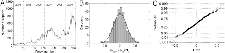
Temporal analysis of the AWD. (A) Weekly number of activity reports in Afghanistan between January 2004 and December 2009 (bin size = 1 w). (B) Distribution of weekly fractional increments in report count in the AWD where N_k denotes the number of report counts at week k. (C) Corresponding normality probability plot. Fourteen points (4.5% of data) were marked as clear outliers as a result of low report count and not used in this analysis.

The field is next decomposed and Eqs. 6 and 8 are applied to finally obtain the random walk model occasionally employed in spatiotemporal studies (29)

[15]

For basis function selection we employed the aforementioned frequency-based approach (see SI Text for complete details). Finally, we chose population density and the distance to the nearest major city as covariates (see SI Text for details on how this choice was made). Inference was carried out using the VB algorithm described above. Full derivatons, algorithmic details, and configuration parameters (priors and stopping conditions), as well as indicative run times, are given in SI Text respectively whilst a detailed simulation study showing the identifiability of the model under flat priors and a comparison with kernel-based estimators (30), is given in SI Text.

Results

Conflict Intensity and Regression Parameters.

State inference leads to broad conclusions to where and how the conflict intensity has increased, decreased or shifted in time. We show the posterior mean intensity at regular intervals in SI Text and also in Movie S1 together with the underlying AWD events at a weekly resolution. The progression of the intensity captures important geographical features of the war scenario. Regions of high intensity in 2009 include Sangin in northern Helmand (see SI Text for a provincial map), one of the most dangerous places in Afghanistan, notorious for thousands of improvised explosive devices and frequent suicide bombings (2). Other regions, such as Kabul, Nangarhar, and Paktya provinces, on the other hand have witnessed high activity throughout the six-year interval. Also very apparent is the emergence in later years of a high intensity ring starting from Kabul extending southwards towards Kandahar, up through Herat, through Balkh and back to Kabul. This roughly elliptical shape corresponds to the country’s ‘ring road’, commonly targeted by insurgent activity and placement of improvised explosive devices (2). We note that a representative spatiotemporal intensity map may also be obtained with the use of standard nonparametric kernel estimators (30), seen in Movie S2.

The regression parameters corresponding to population density and distance to the closest major city were estimated to be 1.97 × 10^-4 ± 6.2 × 10^-6 (2σ) and -0.037 ± 2.1 × 10^-4 respectively. This result reflects the fact that a vast majority of logs in the AWD, as with typical conflict datasets, are present in urban and highly populated areas (7).

Conflict Escalation and Volatility.

A major advantage of the adopted model-based approach is the ability to establish quantitative conclusions on aspects of the conflict scenario other than the intensity. For instance, in the AWD we have modeled the spatially varying escalation of conflict in Afghanistan between 2004 and 2009 through ϑ (Fig. 2) and the volatility of the conflict progression in the same period through the diagonal elements of Σ_Q (Fig. 3).

Fig. 2.

AWD activity growth in Afghanistan. (A) Posterior mean fractional increase in logs per week in the AWD between 2004 and 2009. Only regions with positive overall growth are shown. (B–F left) Spatial map of all events occurring in a square of side 100 km centered on the city under study. (B–F right) Number of weekly events N_k in these regions (-) together with the estimated 90% confidence intervals (green shading).

Fig. 3.

Volatility in conflict events between 2004 and 2009 in the WikiLeaks AWD. Only regions with a high volatility (σ² > 0.055) are shown.

Escalation (or deescalation) may be used to distinguish between event hot spots and growth hot spots. This feature is, in itself, a major advantage over conflict clustering analysis which cannot discern whether a cluster was a one-off, or a sign of a deteriorating situation. In the AWD it is very evident, for instance, that while some of the high growth areas such as Helmand also had an overall high count of events, this was not the general case; for example, Sar-e Pul and Balkh in the north and the Badghis province in the west all had witnessed a modest number of total event count but are seen to have had a significant overall growth in activity throughout the years.

The volatility/predictability of the conflict is also of considerable interest. In our case, a small diagonal value in Σ_Q indicates that based on the data so far the future intensity may be predicted with reasonable accuracy. On the other hand, a large value is a sign of considerable volatility; little can be said about the future. Such inferences are vital for decision purposes—simply stated it might prove a better option to admit a large uncertainty about the future, than to base a policy decision on a highly uncertain prediction. Consider for instance the high volatility on the eastern part of Farah province in western Afghanistan (see SI Text). A subsequent analysis of the video shows spurious clusters emerging in April 2005 and towards the end of 2006, an indication that the conflict dynamics in this part of Afghanistan are relatively hard to predict; even more so than in Sangin which had seen a drastic, but relatively smooth, increase in events in the latter years.

Prediction.

The key advantage of dynamic point process modelling is the ability to make statistical predictions of the system’s behavior for decision making. To illustrate this feature we considered the frequency of incidents by armed opposition groups (AOG) and predicted it in 2010, a year after the termination of the WikiLeaks dataset. AOG activity on a provincial scale was obtained from the Afghanistan NGO Safety Office (ANSO) safety reports^‡. Prediction was carried out by (i) sampling a trajectory z_k through in 2009, (ii) forward simulating each trajectory for 52 weeks (2010) using the generative model with the parameters ϑ, Σ_Q and b set to , 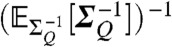and respectively, (iii) integrating the interpolated sample over each ith province to give , (iv) finding the corresponding intensity , (v) averaging the intensity over 52 w invervals to obtain and , (vi) generating two samples N_i,2009 and N_i,2010 from Poisson random variables with intensity and , (vii) predicting a provincial AOG count in 2010, AOG_i,2010, from that in 2009, AOG_i,2009, through the formula

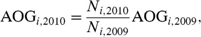[16]

and (viii) repeating (i)–(vii) for N = 2,000 times. Note that although Eq. 16 is a very simple predictor, one which assumes a linear relationship (without offset), it reflects the fact that the frequency of the logs in the WikiLeaks dataset is significantly correlated with the saliency of AOG initiated attacks in Afghanistan, particularly in 2009 (SI Text).

As seen from Fig. 4 A and B, the prediction medians from the model match closely the observed values. In Baghlan, for instance, AOG activity rose by 120% (17.3% using log counts) from 100 incidents in 2009 to 222 in 2010; the model predicted a median 2010 increase of 128% (17.9%) to a count of 228. Badakhshan saw a -19% (-5.5%) growth in 2010; our model predicted a median of -23% (-7.0%) growth. Further, a correlation test between the predicted medians and actual incident count for all 32 provinces gave a Pearson’s correlation coefficient of 0.81 on a linear scale and 0.89 under a log transform (Fig. 4B), showing strong support for prediction capability.

Fig. 4.

Prediction of AOG growth in 2010. (A) Box-and-whisker plots of the predicted log AOG activity in 2010 using 2000 MC runs. For each province, the box marks the first and third quartiles; the median (red line), mean (black circle), and true reported count (green circle) are also given. The whiskers extend to the furthest MC points that are within 1.5 times the interquartile range (≈99% coverage) and the outliers are plotted individually (red cross). (B) Comparison between the median log model prediction and log AOG count in 2010 where the mark number corresponds to the province number denoted in (A). (−) Ideal prediction. (C) Cumulative distribution of growth prediction on a province-by-province basis. The graph shows correct tuning of the model, with approximately x% of provinces lying within the xth percentile of the predictive distribution. (−) True cumulative score. (dotted line) Ideal cumulative score.

Despite this, for some provinces (such as Badghis), the median remains substantially offset from the true value. The disparities are, however, consistent with the predictive distributions. From Fig. 4A it is seen that counts in 62.5% of the predicted provinces lie between the lower and upper quartiles and more importantly all of them lie within the 99% confidence intervals. The same holds for the predicted change in AOG activity in 2010, the distributions of which are given in SI Text. Even here, the model is seen to be well tuned and supply confidence intervals which consistently capture the true activity growth (Fig. 4C).

Thus, although the true count is not always close to the pointwise median predictions, we see that the predictions are accurate in a statistical sense; i.e., the predicted and observed distribution of AOG growth across provinces match closely. Further, the above results were obtained merely from the AWD up to 2009 and did not include any knowledge of events in 2010 such as military plans or deployments/withdrawal of troops. Incorporation of domain knowledge to reduce the predictive variance would, in principle, be straightforward in our model through manipulation of the prior distributions or inclusion of further relevant exogeneous inputs.

Discussion and Conclusions

Our results demonstrate that statistical spatiotemporal modelling can be an extremely valuable tool in the analysis of conflict. The analysis of the AWD data shows that data modelling can yield insights that cannot be achieved by simple visualization or by the use of descriptive statistics. This claim is borne out by the availability of a spatially resolved map of the growth of conflict intensity, as well as the volatility/predictability of the conflict. Furthermore, the availability of statistical confidence intervals associated with all model predictions is an important feature of our modelling framework and a potentially crucial feature for decision making.

The most striking result of our analysis is the ability to accurately predict (in a statistical sense) conflict dynamics for a whole year after the end of the AWD data on which the model was trained. While we do not have a simple mechanism underlying our model, the fact that a latent Gaussian model can produce predictions of this quality cannot be by chance. Intuitively, we believe that the type of conflict we are modelling may be the main reason why our method works. The Afghan conflict is characterized by insurgent movements and qualifies as a case of irregular warfare where activity is only loosely dependent and actioned by a myriad of disparate groups. Some averaging effects may be leading to the Gaussian behavior of the conflict’s intensity, which in turn may be exploited for modelling purposes.

Naturally, as with all modelling techniques, our approach comes also with limitations, as well as benefits. From the technical point of view, reliable parameter estimation in point processes requires a sufficiently large number of events within the region of interest. While it is difficult to put a precise figure to this number, we found that parameter estimation in provinces with fewer event counts than a few dozens a year was extremely difficult. Another limitation may be the suitability of the modelling approach to generic conflict scenarios. Our approach appears to be more suitable for fragmented scenarios such as Afghanistan rather than conventional wars between well organized armies. Finally, we have assumed temporal-invariance of the parameters. Sequential implementations allowing continuous estimation of slowly varying governing parameters are in principle straightforward (11) and offer an attractive way forward to the study of conflict.

In conclusion, the analysis presented in this paper has been made possible by the development of statistical methodologies to handle large scale spatiotemporal datasets. Given the increased availability of such datasets from remote sensing or social networking sources, we envisage that methods such as those used here will become increasingly useful in a number of disciplines.

References

- 1.Raleigh C, Linke A, Hegre H, Karlsen J. Introducing ACLED: an armed conflict location and event dataset. J Peace Res. 2010;47:651–660. [Google Scholar]
- 2.O’Loughlin J, Witmer FDW, Linke AM, Thorwardson N. Peering into the fog of war: the geography of the WikiLeaks Afghanistan war logs, 2004–2009. Eurasian Geogr Econ. 2010;51:472–495. [Google Scholar]
- 3.O’Loughlin J, Witmer FDW, Linke AM. The Afghanistan-Pakistan wars, 2008–2009: micro-geographies, conflict diffusion, and clusters of violence. Eurasian Geogr Econ. 2010;51:437–471. [Google Scholar]
- 4.Gleditsch KS, Weidmann NB. Richardson in the information age: GIS and spatial data in international studies. Annu Rev Polit Sci. 2012;15:461–481. [Google Scholar]
- 5.Bohannon J. Counting the dead in Afghanistan. Science. 2011;331:1256–1260. doi: 10.1126/science.2011.331.6022.331_1256. [DOI] [PubMed] [Google Scholar]
- 6.Haushofer J, Biletzki A, Kanwisher N. Both sides retaliate in the Israeli–Palestinian conflict. Proc Natl Acad Sci USA. 2010;107:17927–17932. doi: 10.1073/pnas.1012115107. [DOI] [PMC free article] [PubMed] [Google Scholar]
- 7.Weidmann NB, Ward MD. Predicting conflict in space and time. J Conflict Resolut. 2010;54:883–901. [Google Scholar]
- 8.Schutte S, Weidmann NB. Diffusion patterns of violence in civil wars. Polit Geogr. 2011;30:143–152. [Google Scholar]
- 9.Zhukov YM. Roads and the diffusion of insurgent violence: the logistics of conflict in Russia’s North Caucasus. Polit Geogr. 2012;31:144–156. [Google Scholar]
- 10.Moeller J, Waagepetersen R. Statistical Inference and Simulation for Spatial Point Processes. Boca Raton: CRC Press; 2004. [Google Scholar]
- 11.Zammit Mangion A, Yuan K, Kadirkamanathan V, Niranjan M, Sanguinetti G. Online variational inference for state-space models with point-process observations. Neural Comput. 2011;23:1967–1999. doi: 10.1162/NECO_a_00156. [DOI] [PubMed] [Google Scholar]
- 12.Zammit Mangion A, Sanguinetti G, Kadirkamanathan V. Variational estimation in spatiotemporal systems from continuous and point-process observations. IEEE T Signal Process. 2012;60:3449–3459. [Google Scholar]
- 13.Wikle CK, Holan SH. Polynomial nonlinear spatio-temporal integro-difference equation models. J Time Ser Anal. 2011;32:339–350. [Google Scholar]
- 14.Cressie NAC, Wikle CK. Statistics for Spatio-temporal Data. New Jersey: Wiley; 2011. [Google Scholar]
- 15.Diggle P, Rowlingson B, Su T. Point process methodology for online spatio-temporal disease surveillance. Environmetrics. 2005;16:423–434. [Google Scholar]
- 16.Brix A, Moeller J. Space-time multi type log Gaussian Cox processes with a view to modelling weeds. Scandinavian Journal of Statistics. 2001;28:471–488. [Google Scholar]
- 17.Rasmussen CE, Williams CKI. Gaussian Processes for Machine Learning. Cambridge, MA: The MIT Press; 2006. [Google Scholar]
- 18.Kot M, Lewis MA, van den Driessche P. Dispersal data and the spread of invading organisms. Ecology. 1996;77:2027–2042. [Google Scholar]
- 19.Wikle CK. A kernel-based spectral model for non-Gaussian spatiotemporal processes. Stat Model. 2002;2:299–314. [Google Scholar]
- 20.Dewar M, Scerri K, Kadirkamanathan V. Data-driven spatiotemporal modeling using the integro-difference equation. IEEE T Signal Process. 2009;57:83–91. [Google Scholar]
- 21.Scerri K, Dewar M, Kadirkamanathan V. Estimation and model selection for an IDE-based spatio-temporal model. IEEE T Signal Process. 2009;57:482–492. [Google Scholar]
- 22.Rodrigues A, Diggle P. A class of convolution-based models for spatiotemporal processes with non-separable covariance structure. Scandinavian Journal of Statistics. 2010;37:553–567. [Google Scholar]
- 23.Higdon D. A process convolution approach to modelling temperatures in the North Atlantic ocean (with Discussion) Environ Ecol Stat. 1998;5:173–190. [Google Scholar]
- 24.Bracewell R. in The Fourier Transform & its Applications. 3rd Ed. Singapore: McGraw-Hill; 2000. p. 122. [Google Scholar]
- 25.Freestone DR, et al. A data-driven framework for neural field modeling. NeuroImage. 2011;56:1043–1058. doi: 10.1016/j.neuroimage.2011.02.027. [DOI] [PubMed] [Google Scholar]
- 26.Beal MJ. University College London, United Kingdom: Gatsby Computational Neuroscience Unit; 2003. Variational Algorithms for Approximate Bayesian Inference. PhD thesis. [Google Scholar]
- 27.Smidl V, Quinn A. The Variational Bayes Method in Signal Processing. New York: Springer Verlag; 2005. [Google Scholar]
- 28.Jazwinski AH. Stochastic Processes and Filtering Theory. London: Academic Press; 1970. [Google Scholar]
- 29.Stroud JR, Mueller P, Sanso B. Dynamic models for spatiotemporal data. J R Stat Soc B Stat Met. 2001;63:673–689. [Google Scholar]
- 30.Diggle P. A kernel method for smoothing point process data. Appl Stat. 1985;34:138–147. [Google Scholar]
Associated Data
This section collects any data citations, data availability statements, or supplementary materials included in this article.