

Summary
1. Environmental variables are often used as indirect surrogates for mapping biodiversity because species survey data are scant at regional scales, especially in the marine realm. However, environmental variables are measured on arbitrary scales unlikely to have simple, direct relationships with biological patterns. Instead, biodiversity may respond nonlinearly and to interactions between environmental variables.
2. To investigate the role of the environment in driving patterns of biodiversity composition in large marine regions, we collated multiple biological survey and environmental data sets from tropical NE Australia, the deep Gulf of Mexico and the temperate Gulf of Maine. We then quantified the shape and magnitude of multispecies responses along >30 environmental gradients and the extent to which these variables predicted regional distributions. To do this, we applied a new statistical approach, Gradient Forest, an extension of Random Forest, capable of modelling nonlinear and threshold responses.
3. The regional‐scale environmental variables predicted an average of 13–35% (up to 50–85% for individual species) of the variation in species abundance distributions. Important predictors differed among regions and biota and included depth, salinity, temperature, sediment composition and current stress. The shapes of responses along gradients also differed and were nonlinear, often with thresholds indicative of step changes in composition. These differing regional responses were partly due to differing environmental indicators of bioregional boundaries and, given the results to date, may indicate limited scope for extrapolating bio‐physical relationships beyond the region of source data sets.
4. Synthesis and applications. Gradient Forest offers a new capability for exploring relationships between biodiversity and environmental gradients, generating new information on multispecies responses at a detail not available previously. Importantly, given the scarcity of data, Gradient Forest enables the combined use of information from disparate data sets. The gradient response curves provide biologically informed transformations of environmental layers to predict and map expected patterns of biodiversity composition that represent sampled composition better than uninformed variables. The approach can be applied to support marine spatial planning and management and has similar applicability in terrestrial realms.
Keywords: beta diversity, community ecology, conservation, environmental surrogates, habitat suitability modelling, spatial planning and management, species distribution modelling
Short abstract
Gradient Forest offers a new capability for exploring relationships between biodiversity and environmental gradients, generating new information on multispecies responses at a detail not available previously. Importantly, given the scarcity of data, Gradient Forest enables the combined use of information from disparate data sets. The gradient response curves provide biologically informed transformations of environmental layers to predict and map expected patterns of biodiversity composition that represent sampled composition better than uninformed variables. The approach can be applied to support marine spatial planning and management and has similar applicability in terrestrial realms.
Introduction
Many nations now embrace a broader ecosystem‐based approach to management (EBM, Garcia et al. 2003) to address concerns about sustainability in response to increasing anthropogenic pressures on the marine environment. EBM includes conservation of biodiversity and strategies such as marine spatial planning and marine protected areas (MPAs). As on land, environmental mapping is a necessary foundation for EBM and MPA planning (Cogan et al. 2009). However, the marine environment is comparatively inaccessible and expensive to observe and, as a consequence, biological survey data are often sparse. Given national policy requirements to implement EBM, the need for bioregional mapping has often been met using surrogates such as geological or other physical data (reviewed in McArthur et al. 2010) presented in hierarchical classifications (e.g. Greene et al. 1999), expert‐derived regionalizations (e.g. Thackway & Cresswell 1998), or unsupervised clusterings (e.g. Whiteway et al. 2007). Surrogate‐based maps are assumed to be representative of biological patterns because an extensive literature on ‘species–environment relationships’ (SER) has correlated biological patterns with factors such as depth, substratum, light and others (e.g. Gray 1974; Snelgrove & Butman 1994; Levin et al. 2001). However, in developing hierarchical or categorical mapping schemes, SERs, if used, typically are considered only qualitatively or indirectly. There is no certainty that the relative weighting of environmental variables in the mapping scheme is proportional to the influence on biological patterns or that category boundaries imposed on environmental gradients coincide with substantive changes in assemblage composition. A more biologically relevant approach is needed to directly integrate quantitative and continuous biological response information into bioregional mapping based on environmental data. More fundamentally, some ecological theories hypothesize that species distributions, abundances and compositions are determined by environmental tolerances and resource preferences, while others emphasize alternative drivers such as historical events, connectivity, recruitment and species interactions. A more comprehensive approach to quantifying multispecies responses to environmental gradients will therefore make an important contribution to the basic understanding of the drivers of biodiversity composition patterns (‘beta diversity’, Whittaker 1972), as proposed by Legendre, Borcard & Peres‐Neto (2005).
Several existing methods can link biodiversity patterns with environmental data for ecological and management applications. For example, constrained canonical correspondence analysis (CCA, ter Braak 1986) uses a multiple linear regression framework to fit an ordination of chi‐squared distances of site‐by‐species data as a function of linear combinations of environmental variables; and generalized dissimilarity modelling (GDM, Ferrier et al. 2007) uses a generalized linear modelling framework to fit Bray–Curtis dissimilarities between sites as a linear combination of spline functions of environmental differences between sites. To more fully explore the patterns and magnitude of changes in species composition along environmental gradients, we applied a new more flexible nonparametric approach, Gradient Forest (http://r‐forge.r‐project.org/projects/gradientforest/), developed by Ellis, Smith & Pitcher (2012) for our application here. The new method extends Random Forest (Breiman 2001), which fits an ensemble of regression tree models between individual species abundance and environmental variables. From these, Gradient Forest accumulates standardized measures of species changes along the gradients for multiple species and uses them to build empirical nonlinear functions of compositional change for each variable. Thus, Gradient Forest is a new exploratory tool for ecological investigations, the statistical foundation for which is presented in Ellis, Smith & Pitcher (2012) who also compare technical aspects of this new method with those of some existing methods.
Here, we present the first ecological application of Gradient Forest, analysing multiple large‐scale seabed biodiversity survey data sets with the overall goal of contrasting and interpreting compositional responses along environmental gradients among three different marine regions. The standard Random Forest method can address our first two specific objectives: (1) to quantify the overall extent to which environmental variables can predict distribution patterns; and (2) to quantify the importance of each variable to the predictions (but see methods re conditional importance). Gradient Forest adds the tools necessary to address our next two objectives: (3) to explore the empirical shape and magnitude of changes in composition along environmental gradients; and (4) to identify any critical values along these gradients that correspond to threshold changes in composition. The consistency of these patterns and thresholds across regions, which is of particular interest in ecology and its applications, is examined herein. We also illustrate how Gradient Forest outputs, having integrated biological information, provide improved use of surrogates for bioregional mapping applications with an example map for one of our study regions.
Materials and methods
Regional Biological Data Sets and Environmental Variables
We collated biological and environmental data sets from three regional‐scale (2–5 × 10⁵ km2) marine ecosystems: the continental shelf of the Great Barrier Reef system (GBR), the Gulf of Maine area (GoMA) and the deep Gulf of Mexico (DGoMx) (Table 1). The biological data sets comprised site‐by‐species abundance data from seabed trawl, epi‐benthic sled and/or grab/core surveys considered representative for characterizing assemblages at meso‐scales (10s km) (see Appendix S1 in Supporting Information for details and data sources). All data were standardized for sampling effort and log(x + min(x,x > 0)) transformed, and surveys of different device types, seasons or time periods were analysed separately. The physical, geological and environmental data sets comprised the most comprehensive suite to date of available marine variables considered potentially important for influencing marine species distributions and composition at meso‐scales, including attributes of bathymetry, sediments, water chemistry and ocean colour (see Appendix S2 in Supporting Information for code definitions, descriptions and data sources). Values of the environmental variables were matched by spatial position to the sites sampled for biological data – herein, these are called predictors and their observed ranges are called gradients.
Table 1.
Basic statistics for regional study areas and data sets (#sps +ve R 2 = number of species with model having a positive R 2. See Appendix S1 for details and sources of biological data sets)
| GBR | GoMA | DGoMx | ||||
|---|---|---|---|---|---|---|
| Sled | Trawl | Grab | Trawl | Core | Trawl | |
| Area ’000 km2 | c. 200 | c. 250 | c. 500 | |||
| Depth range m | 5–105 | 7–603 | 213–3732 | |||
| #Predictors | 29 | 29 | 26 | 27 | 20 | 20 |
| #Data sets | 1 | 1 | 1 | 4 | 3 | 2 |
| #Sites | 1189 | 458 | 478 | 5917 | 85 | 78 |
| #Species | 4240 | 2899 | 315 | 297 | 2553 | 637 |
| #sps analysed | 616 | 357 | 53 | 157 | 419 | 232 |
| #sps +ve R 2 | 405 | 272 | 25 | 127 | 254 | 166 |
| Data type | Weight | Weight | Count | Count | Count | Count |
| Mean R 2 (range) | 0·13 (0–0·52) | 0·22 (0–0·67) | 0·21 (0–0·63) | 0·29 (0–0·78) | 0·22 (0–0·72) | 0·35 (0–0·85) |
We selected available environmental variables relevant to the application of surrogates for mapping biodiversity patterns at regional management scales. To be useful as a surrogate in this context, the predictor variables must be readily available as full coverage layers at the scales of interest. This goal may differ from those of purely ecological studies, where fine‐scale habitat variables may be collected along with biological data, at the scale of the sites, but these variables may not be available beyond the sampled sites for larger‐scale prediction. Similar considerations affected temporal aspects of the data. Temporally varying environmental data were summarized as a climatic mean and variation; where possible, to coincide with broad periods when biological surveys occurred to minimize temporal mismatch. While these broad spatial and temporal data sets may not account for some fine‐scale biological responses, we emphasize that we wished to assess the performance of regional‐scale surrogates for mapping relatively stable patterns of biodiversity.
Many of the predictors were interpolated in various ways to obtain full coverage. This inextricably intertwines space and environment; however, space was not explicitly included as a predictor. Spatial nonindependence was not considered an issue because sites were located sufficiently far apart to ensure a high likelihood of spatial independence of observations in each survey. For example, the GBR sites averaged c. 13 km apart compared with earlier variogram and correlogram studies that indicated local autocorrelation ranged to about 4 km (Pitcher et al. 2007). Similarly, Kraan et al. (2010) found that residual autocorrelation was negligible beyond c. 2·5 km. Further, supplementary analyses of the GBR data sets incorporating geographic distance confirmed that space was not an important contributor (see Discussion).
Statistical Approach
Gradient Forest has two components. The first is an extended version of the Random Forest implementation of R Development Core Team (2011) package randomForest (Liaw & Wiener 2002). This partitioning method works by finding, at each tree branch, the split value on one of the predictors that minimizes the sums‐of‐squares of the species abundance in the child branches, that is, maximizes the fit improvement; but to avoid the instability of individual trees, a forest of trees (500, in our case) is fitted. Each tree in the forest is fitted to a random sample (0·632, on average) of the observations (the ‘in‐bag’), each split is selected from a different random subset of one‐third of the predictors, and the performance of each tree is cross‐validated against the remaining ‘out‐of‐bag’ observations. We applied the extended version (package extendedForest), which additionally retains all split values and fit improvements for each species, in each survey data set that had sufficient frequency of occurrence (Table 1; Appendix S1).
The overall predictive performance of the forest was evaluated by the proportion of out‐of‐bag data variance explained (R 2) for each species, which is a robust estimate of generalization error (objective 1, output 1). The importance of each predictor to model accuracy was assessed by quantifying the degradation in performance when each predictor was randomly permuted (objective 2, output 2). However, where predictors are correlated, as in our data sets, randomForest’s standard marginal importance yields inflated measures of importance. Alternatively, extendedForest takes a conditional approach (Ellis, Smith & Pitcher 2012), where each predictor was permuted only within blocks of observations defined by splits in the given tree on any other predictors correlated above a specified threshold (r > 0·5), up to a maximum number of splits (floor(log2(n × 0·368/2)), where n = number of sites). Conditional importance is more robust than marginal importance, nevertheless, correlated predictors can be truly disentangled only by orthogonal experimentation – infeasible at large regional scales.
The second component, package gradientForest (Ellis, Smith & Pitcher 2012), collated the numerous split values along each gradient and their associated fit improvements that were retained by extendedForest, for each predictor in each tree and each forest. This information was then used to construct empirical nonlinear functions of compositional change along each environmental gradient for the entire assemblage (objectives 3 and 4) as follows. For each species, the split improvements were standardized by the density distribution of the observed values of each predictor, to control for nonuniform sampling along the gradients. The standardized splits were then normalized to predictor importance and predictor importances were normalized to species R 2. The standardized and normalized split importances for all species within a survey data set were then combined along each gradient. Thus, each split improvement was re‐expressed in terms of its contribution to total variance explained by the predictors and each species contributed to the quantification of compositional change in proportion to its variance explained by the predictors. The location and magnitude of compositional change along each predictor gradient for each survey was quantified by frequency distributions of the combined splits (output 3). The cumulative compositional change along each gradient (in R 2 units) was quantified by aggregating the normalized splits as cumulative distributions. These cumulative importance curves were plotted for each species and for the aggregated composition of each survey (outputs 4 and 5).
The results from each within‐region survey‐type were combined, using a common density standardization for each predictor in each region, based on the combined density distribution of the observed values of the predictors across all within‐region survey‐types. The standardized splits were normalized and aggregated as above and the cumulative curves plotted to represent overall within‐region compositional change along each gradient. These combined cumulative importance curves from all regions were also plotted together, for each predictor, to facilitate the cross‐regional contrasts that were the overall goal of this study.
Results
In this study, we describe the ecological information available from the outputs of Gradient Forest, beginning with detailed results for selected predictors in the GBR epi‐benthic sled data set. We then compare and contrast key results from the three regional ecosystems, focussing on the degree of influence of environmental variables and interpretation of the shape and magnitude of compositional changes along their gradients. Detailed description of the within‐region biological results will be the focus of separate regional publications. Nevertheless, for completeness, the full results for all survey data sets, each matched with up to 29 regional environmental predictors, are presented in Appendix S3 in Supporting Information.
GBR Epi‐Benthic Sled Patterns
Objective 1: Performance: The suite of environmental variables predicted a relatively modest fraction of the variation in biomass distributions of GBR epi‐benthic sled species (Table 1, mean R 2 and range, output 1) for which these variables had at least some predictive capacity (positive R 2 in Table 1). Predictive performance may have been compromised by factors such as sampling variability, diurnal, tidal, lunar and seasonal cycles, weather and other ecological processes (Pitcher et al. 2007).
Objective 2: Predictor Importance: The most important predictors for these species were sediment grain size fractions, sediment carbonate composition and tidal current stress (Fig. 1, output 2). The importance of these factors for driving distributions of benthic biota is well known (Gray 1974; Snelgrove & Butman 1994) and these results provide corroboration at large regional scale. Bottom‐water chemistry and nutrients were of intermediate importance, as were depth and satellite‐sensed predictors. Often, seasonal ranges (sr) of predictors were more important than their averages (av), suggesting that environmental variability may drive distributions along with mean climate. For example, in the case of bottom‐water oxygen, high seasonal range may be indicative of stratification and seasonally low oxygen levels that may exclude active species. Aspect (the direction of seabed slope) was the least important (Fig. 1).
Figure 1.
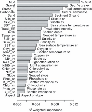
Overall conditional importance of environmental variables for predicting distributions of GBR epi‐benthic sled species, calculated by weighting the species‐level predictor importance by the species R 2 and then averaging (av = annual average; sr = seasonal range; see Appendix S2 for full descriptions of predictors).
Objectives 3 and 4: Gradient Responses and Thresholds: The frequency distributions of split importances (output 3) show that changes in the GBR sled assemblage along environmental gradients were nonuniform. For example, along the sediment mud gradient, many important splits occurred in the range c. 0–20% mud (Fig. 2a, grey histogram), indicating that large changes in species abundance and composition corresponded with small changes in mud content. In the range c. 25–100% mud, splits had low importance, indicating relatively little compositional change across this broad range of mud content. Most sites sampled on the GBR shelf had low mud content (Fig. 2a, red ‘density of data’ line); because of this bias we also indicate the expected density of splits had the mud gradient been sampled with uniform density (Fig. 2a, blue line = ratio of observed density of splits (black line) standardized by the data density). Locations on the gradient where the splits density was greater than data density (ratio > 1, Fig. 2a) indicate higher relative importance for compositional change. Similarly, along a gradient of tidal current stress, locations of high relative rates of assemblage change were around c. 0·4 and c. 0·9 Nm−2 (Fig. 2a, blue line), corresponding to thresholds where currents were strong enough to scour away fine sediments exposing harder or consolidated substrata suitable for the attachment of large sessile fauna. This information on rates of compositional change (Fig. 2a) has important applications for identifying category boundaries on gradients where GIS‐based classification approaches are used for habitat mapping.
Figure 2.
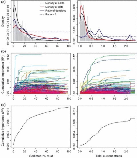
Key graphical outputs of Gradient Forest for GBR epi‐benthic sled along gradients of sediment % mud content and tidal current stress. (a) Splits location and importance on gradient (histogram), density of splits ( ) and observations (
 ) and ratio of splits standardized by observation density (
 ). Each distribution integrates to predictor importance (as per Fig. 1). Ratios >1 indicate locations of relatively greater change in composition. (b) Cumulative distributions of standardized splits importance for each species scaled by R
2; each line denotes a separate species. (c) Cumulative importance curves showing overall pattern of compositional change (R
2) for all species. For other gradients, see Figs S3‐3·1, S3‐4·1 and S3‐5·1 in Appendix S3.
). Each distribution integrates to predictor importance (as per Fig. 1). Ratios >1 indicate locations of relatively greater change in composition. (b) Cumulative distributions of standardized splits importance for each species scaled by R
2; each line denotes a separate species. (c) Cumulative importance curves showing overall pattern of compositional change (R
2) for all species. For other gradients, see Figs S3‐3·1, S3‐4·1 and S3‐5·1 in Appendix S3.
The standardized and accumulated split importance values show the shapes of cumulative change in abundance of each species (Fig. 2b, output 4). Changes for individual species varied in magnitude and threshold values along these gradients, and those contributing to overall compositional change can be identified. For example, a number of species changed substantially between 0 and 10% mud and several others changed quite rapidly at c. 20% mud (Fig. 2b). Normalizing all standardized splits for all species by R 2 and accumulating provides the overall assemblage importance curves (Fig. 2c, output 5) that relate compositional change to each environmental gradient. In these nonlinear curves, shallow slopes indicate low rates of change in species composition, whereas steep slopes indicate high rates, with thresholds corresponding to more pronounced transitions between assemblages.
Regional Patterns and Contrasts
Objective 1: Performance: Abundance patterns in the GoMA and DGoMx data sets tended to be predicted better by the environmental variables than in the GBR. In all regions, the trawl‐sampled species were predicted better than those sampled with smaller devices (Table 1; Appendix S3‐1), possibly because the larger area sampled by trawls reduced data variability.
Objective 2: Predictor Importance: The rank‐order importance of predictors differed among the three regions (Table 2) but was relatively consistent between sampling devices within regions. Compared with the GBR, depth was important in both GoMA and DGoMx and spanned a broader range, suggesting that the gradient range of a predictor may influence its importance outcome. Also unlike in the GBR, in both GoMA and DGoMx water column parameters were more important predictors of seabed fauna. For example, remotely sensed SST and chlorophyll – indicative of circulation patterns, water column mixing and food supply to the benthos (Pettigrew et al. 1998; Thomas, Townsend & Weatherbee 2003) – were important in GoMA, as was exported particulate organic carbon (E.POC) in DGoMx (Wei et al. 2010). Seabed temperature (Temp_av) was also important in both regions and is known to influence trawled fish distributions in GoMA (Perry & Smith 1994). Salinity was moderately important in GoMA and highest ranked in DGoMx where it may indicate different vertical water masses (e.g. Jochens & DiMarco 2008). The force of tides was of high importance in the GBR and in the GoMA, both tidal and wind stress (Stress_T and Stress_tW) were of moderate importance and are known to influence biota in this region (Kostylev et al. 2005). Topographic predictors (e.g. slope, aspect, complexity and BPI) were unimportant in all regions; however, these had a narrow range at sites that could be sampled by extractive devices. Hard, topographically complex habitats are known from optical sampling to have biotic compositions that differ from sedimentary habitats (Kostylev et al. 2001; Pitcher et al. 2007) and results from analyses of such data may show greater importance of topography.
Table 2.
Rank‐order conditional importance for each predictor, after averaging over species weighted by R 2 within each region, by sampling device (see Appendix S2 for definitions and descriptions of predictors)
| GBR | GoMA | DGoMx | |||
|---|---|---|---|---|---|
| Sled | Trawl | Grab | Trawl | Core | Trawl |
| Mud | Mud | SST_av | SST_av | Salin_av | Salin_av |
| Gravel | Carbonate | Depth | Depth | Depth | Depth |
| Stress_T | Stress_T | Strat_sum | Temp_av | E.POC_av | Temp_av |
| Carbonate | Trawl_Eff | Sand | Chlor_av | Temp_av | Temp_sr |
| Sand | Depth | Chlor_sr | Salin_av | Temp_sr | E.POC_av |
| Silic_sr | Sand | B_Irr_av | Stress_tW | Oxyg_av | Salin_sr |
| Silic_av | Silic_av | Gravel | Stress_T | E.POC_sr | SST_av |
| SST_av | Salin_sr | Stress_tW | SST_sr | Salin_sr | K490_sr |
| Trawl_Eff | Salin_av | B_Irr_sr | B_Irr_sr | K490_av | Oxyg_av |
| Depth | SST_av | Chlor_av | B_Irr_av | NPP_av | SST_sr |
| Temp_av | SST_sr | Mud | Mud | Mud | Mud |
| Salin_sr | Gravel | SST_sr | Temp_sr | Slope | Sand |
| Salin_av | Temp_av | Salin_av | Gravel | Sand | NPP_sr |
| SST_sr | Silic_sr | Stress_T | Chlor_sr | Chlor_av | Chlor_sr |
| Oxyg_sr | Oxyg_sr | Oxyg_av | K490_av | SST_av | E.POC_sr |
| Temp_sr | Temp_sr | K490_sr | Sand | SST_sr | Slope |
| Oxyg_av | Nitr_av | Temp_av | Salin_sr | NPP_sr | K490_av |
| Nitr_av | Oxyg_av | Stratif_av | K490_sr | K490_sr | Chlor_av |
| K490_sr | K490_sr | K490_av | Silic_av | Chlor_sr | NPP_av |
| K490_av | Nitr_sr | Temp_sr | Strat_sum | Aspect | Aspect |
| Chlor_av | B_Irr_av | Phos_av | Nitr_av | ||
| Nitr_sr | K490_av | Slope | Stratif_av | ||
| Slope | Slope | Aspect | Phos_av | ||
| Phos_sr | B_Irr_sr | BPI | Slope | ||
| B_Irr_av | Chlor_sr | Complex | Aspect | ||
| Chlor_sr | Phos_av | Complex | |||
| Phos_av | Chlor_av | BPI | |||
| B_Irr_sr | Phos_sr | ||||
| Aspect | Aspect | ||||
Objectives 3 and 4: Gradient Responses and Thresholds: The cumulative importance curves for survey‐types, some combined across multiple data sets within regions, plotted together for all regions (Fig. 3), show strong contrasts in compositional responses to environmental gradients among regions. The results for selected predictors are presented and discussed in the following paragraphs in decreasing order of overall importance (per Fig. 3); regional contrasts in responses along 25 environmental gradients, including seasonal ranges, are presented in Fig. S3‐7·1 in Appendix S3.
Figure 3.
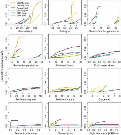
Cumulative importance curves (R 2) for selected predictors available in two or more regions, in order of overall importance, showing contrasting compositional responses along gradients among regions (av = annual average; see Appendix S2 for full descriptions of predictors; see Fig. S3‐7·1 in Appendix S3 for other predictors, including seasonal ranges).
Along the depth gradient, most compositional changes occurred shallower than 300–800 m (Fig. 3); a range where many physiologically important predictors have greatest variation. The DGoMx samples extended deeper by another 3000 m, over which composition continued to change, increasing the overall importance of depth in that region. In GoMA, depths of 50–150 m and c. 350 m corresponded with important compositional changes. Depth per se was unlikely to be directly influential but was highly correlated with about one‐third of the other predictors, including those considered influential, such as salinity, temperature, oxygen and light (Snelgrove & Butman 1994), and exported carbon (Wei et al. 2010). The assessment of predictor importance by conditional permutation aimed to account for such correlations, and the remaining importance of depth may be indicative of other influential factors correlated with depth and not accounted for by other variables, such as boundaries between different water masses with different conditions, circulation patterns and species pools.
Several lines of evidence indicated that the major broad‐scale faunal changes in the regional data sets were linked with different water masses. Along the salinity gradient (Fig. 3), the DGoMx composition changed very sharply at 35·1–35·2‰, possibly reflecting limited exchange between Antarctic Intermediate Water transported into the Gulf of Mexico by the Loop Current beneath a warmer high‐salinity water mass (Jochens & DiMarco 2008). In the GoMA, composition changed more gradually over a c. 4‰ range of salinity (Fig. 3) with trawl composition changing more steeply at c. 34–35‰, corresponding to the transition to upper slope water at the shelf edge (Flagg 1987) and in deeper waters within the interior of the Gulf (Ramp, Schlitz & Wright 1985). A small step change in the GBR data sets at c. 36·2‰ also corresponded with the shelf edge. Along the SST gradient, the GoMA seabed assemblage changed very steeply at c. 12 °C (Fig. 3), where warmer northwards‐flowing Gulf Stream‐influenced waters in southern offshore areas transition to cooler southwards‐flowing boreal‐influenced waters north and inshore. This steep change corresponds closely with the well‐known provincial transition in the region (Briggs 1974), which reflects patterns of connectivity for sessile and sedentary benthic biota (Jennings et al. 2009). In contrast, SST was of moderate to low importance in the GBR and DGoMx. In DGoMx, SST corresponded with other depth‐correlated gradients, and in the GBR, a slightly steeper change at c. 24·5 °C separated the southernmost section, where some subtropical species occur, from more tropical assemblages to the north. Along the seabed temperature gradient (Fig. 3), the DGoMx and GoMA trawl data sets showed strong compositional changes through c. 7–10 °C; a range known in the GoMA to influence the distribution of several fish species (Perry & Smith 1994) and benthic assemblages (Mountain, Langton & Watling 1994). The GBR composition changed much less over a similarly wide range of much warmer seabed water temperature.
Along the sediment mud gradient, the GBR trawl and sled compositions changed more than the other regions (Fig. 3), with greatest change at 0–20% as noted earlier. The GoMA trawl composition changed more gradually, with a slight step change at c. 15% mud. The other data sets showed less overall response, with modest changes where mud content was high. Along the tidal stress gradient (Fig. 3), the composition of both GoMA survey‐types tended to have small step changes at values similar to the GBR data sets, with similar overall importance (Fig. 3; see also subsections S3‐3 and S3‐5 within Appendix S3).
On the oxygen gradient (Fig. 3), the most important changes occurred at c. 4–5 ml l−1. While this range is above the threshold commonly accepted for hypoxic conditions (c. 2 ml l−1), sublethal effects can occur at higher oxygen levels, including distributional responses (Vaquer‐Sunyer & Duarte 2008). In this respect, a threshold for oxygen in the DGoMx trawl composition (at c. 5 ml l−1) is greater than that for the box core (at c. 3 ml l−1), possibly indicating preference for higher oxygen among active trawled species compared with sedentary species in the cores (cf. Vaquer‐Sunyer & Duarte 2008). Along the relative benthic irradiance gradient (Fig. 3), the GoMA composition showed a step change at very low light levels separating the few sites located in shallow water from the remainder. Along the chlorophyll and light‐attenuation gradients (Fig. 3), the GoMA trawl composition changed most, corresponding to higher productivity coastal and inshore and Georges Bank sites vs. other areas (Thomas, Townsend & Weatherbee 2003).
Discussion
Gradient Forest provides several new benefits for exploring multi‐species composition. It inherits the strengths of univariate Random Forest, including predictive performance, automated model selection, accounting for complex interactions, few data assumptions and does not require specialist model building skills (for a full discussion, see Ellis, Smith & Pitcher 2012). Gradient Forest extends these strengths to multiple species, providing a nonlinear and highly flexible method for quantifying details of compositional change along gradients, including thresholds. Further, because dimensionless R 2 is used to quantify change, information from multiple data sets can be combined, even if disparate sampling methods have been used. Thus, Gradient Forest uniquely is able to identify steep compositional thresholds along gradients; for example, on salinity in DGoMx, on SST in GoMA and on mud and tidal stress in the GBR. Nevertheless, like all existing methods used for similar purposes, Gradient Forest is correlative and the results do not imply causal relationships.
The approach is also not guaranteed to have high performance if SER are weak or sampling variability is great, despite the power of the underlying Random Forests. In our analyses, the abundance of almost one‐third of species showed no predictable relationship with the environmental variables and for those species that did these variables predicted an average of only 13–35% of the variation in their abundance distributions (R 2, Table 1) but >50% for some species in all data sets (maximum = 85%). Our use of broad spatial and temporal scale environmental layers as predictors, rather than fine‐scale factors, may have contributed to the low variance explained for most species and is an important reality check about the use of such surrogates. Nevertheless, our results are not unusual for marine benthic studies; for example, generalized linear models of 850 species in the GBR data set performed similarly (Pitcher et al. 2007) and other model comparison studies (e.g. Elith et al. 2006) found that only half of the species analysed had useable models and few had strong models, even for tree‐ensemble models that performed best. Further, our R 2 results are for cross‐validated prediction performance on out‐of‐bag samples, which is more conservative than explained variation of fit to in‐bag samples. In addition, we analysed abundance data because it incorporates more detailed compositional information, but also more variability, within survey data compared with presence/absence data. Finally, although the environmental variables were imprecise for predicting local abundance, at larger scales the effects of local heterogeneity are averaged out and broad patterns become more predictable (Wiens 1989); hence, environmental surrogates remain useful for broad‐scale bioregionalization.
Clearly, however, the environment is often not the primary driver of species distributions and compositions. We note that spatial processes per se were not important at the scales analysed (e.g. analyses of the GBR data set, using GDM with and without geographic distance, indicated that space alone – over and above spatially structured environment – explained <0·1% of deviance; C. R. Pitcher, unpublished data). Our results support the likelihood of multiple drivers of species distributions contributing to beta diversity patterns; some species appear to be strongly environmentally driven, whereas others only partly or not at all. The distributions of these latter species may be driven by other processes such as missing or finer‐scale predictors, historical events, connectivity, recruitment variability and species interactions (e.g. predation, competition and facilitation). Spatial planning and management activities need to consider these other processes that also drive biodiversity patterns.
Combinations of environmental predictors were associated with biodiversity composition patterns, and their relative importance differed among regions. Although we collated extensive regional data sets as available for these comparisons, they were not fully orthogonal in terms of gear types (e.g. benthic sled was available only for the GBR) or the groups of biota identified (e.g. primarily fishes in GoMA trawls, whereas DGoMx trawls included many invertebrates and GBR sled samples also included plants). These differences almost certainly contributed to the contrasting shapes of compositional responses we observed among the three regions. The biggest differences, however, were that both North American study regions spanned provincial transitions (vertically in GoMx, mostly horizontally in GoMA), whereas the GBR did not. The substantial compositional changes across these transitions were detected by sharp thresholds located on gradients of primarily salinity or SST, and depth, which were surrogates for different water masses. The limited consistency among responses observed here, suggest there may be limited scope for extrapolating biophysical relationships beyond the source region of the informing data sets.
Within regions, the cumulative importance curves that quantify gradient response shapes and thresholds can be used as biologically informed transformations of broad‐scale environmental data layers to map expected patterns of biodiversity composition. The procedure for this follows the example provided by Pitcher, Ellis & Smith (2011). After transformation by the cumulative importance curves, the principal components of the transformed predictors provide a multidimensional representation of variation in composition that is constrained by relationships between the species and their environment. This approach is akin to community analyses commonly practiced in ecology (e.g. constrained CCA, ter Braak 1986), but involves a flexible nonlinear method rather than linear models. Consequently, the Gradient Forest outputs represented biodiversity composition patterns c. 25–50% better than could be achieved with uninformed, standardized environmental variables (Appendix S4 in Supporting Information). An example map for the GBR (Fig. 4) shows a continuous representation of biodiversity composition patterns encompassed by the first two dimensions of a biologically transformed environment space. If required, this continuous representation can be clustered to map expected assemblages.
Figure 4.
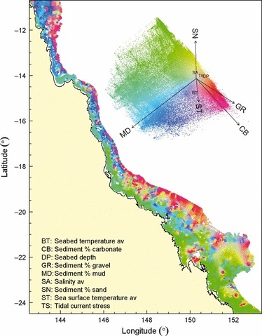
Map of transformed environmental variables, following Gradient Forest analyses and combining results for the GBR sled and trawl data, representing the first two dimensions of expected continuous patterns of composition for seabed biodiversity. The biplot of the first two principal dimensions of the biologically transformed environment space provides a colour key for the compositional variation, with vectors indicating the direction and magnitude of major environmental correlates.
Maps representing expected patterns of regional biodiversity composition have important applications for EBM, including marine spatial planning and conservation planning such as MPAs. Characterizing and mapping the marine realm for these purposes, using robust statistical techniques such as Gradient Forest, which can directly integrate quantitative biological response information into mapped environmental variables, is a necessary initial approach that will assist the current global need for precautionary management. Such techniques can also identify areas of prediction uncertainty and data gaps to target and facilitate sampling design, including stratification, of future marine biodiversity surveys. In these marine applications, as for terrestrial environments, there is a need to maximize the utility of existing biological and environmental data sets given the cost of new surveys. This utility is where Gradient Forest’s ability to integrate quantitative results across multiple disparate surveys – contemporary and/or historical, including those that used different sampling methods – is of great value, with wider applicability beyond our marine example.
Gradient Forest provides new detail about SER and compositional changes along gradients, relevant to hypotheses about the drivers of beta diversity and for predicting patterns of biodiversity composition. The strengths and new capabilities of Gradient Forest complement those of existing methods that explore relationships between composition and environment, such as constrained CCA and GDM. These three methods are difficult to compare directly because of their contrasting techniques and different diagnostics; also there is no standard measure of compositional patterns to serve as a benchmark. The compositional patterns obtained from mapping the Gradient Forest results for the GBR here were similar to patterns obtained from comparable mapping of results from constrained CCA and GDM analyses (C. R. Pitcher, unpublished data), but a full comparison is beyond the scope of this study and detailed comparisons on the same data sets would be valuable.
Our first analyses in three large, strongly contrasting marine regions did not reveal ‘global’ consistencies in compositional responses along environmental gradients that may have led to generalizable transformation functions to improve first‐order bioregional mapping in jurisdictions lacking comprehensive biological survey data. However, our study presented a very harsh test. Further analyses of additional data sets, including multiple sampling devices, biotic groups, environmental gradients and regions are required for filling gaps in data types and predictor ranges to broaden the information available on biophysical relationships for marine assemblages. Accumulation of these additional results will further our understanding of the drivers of compositional change along environmental gradients and their use as surrogates for biodiversity.
Supporting information
Appendix S1. Descriptions of regional biological data sets.
Appendix S2. Descriptions of regional environmental variables.
Appendix S3. Complete graphical results for three marine regions.
Appendix S4. Quantifying performance of biologically informed mapping.
As a service to our authors and readers, this journal provides supporting information supplied by the authors. Such materials may be re‐organized for online delivery, but are not copy‐edited or typeset. Technical support issues arising from supporting information (other than missing files) should be addressed to the authors.
Supporting info item
Supporting info item
Supporting info item
Supporting info item
Acknowledgements
For use of survey data, we thank the U.S. Northeast Fisheries Science Centre (National Marine Fisheries Service) and the Minerals Management Service (now Bureau of Ocean Energy Management, U.S. Department of the Interior), Fisheries and Oceans Canada, and the Census of Marine Life (CoML) Gulf of Maine Area Program (GoMA). This work is the product of a CoML cross‐program synthesis project (2008–2010) supported by the Alfred P. Sloan Foundation, and by the authors’ institutions: CSIRO Australia, Fisheries and Oceans Canada through its Ecosystem Research Initiative, University of Southern Maine, Texas A&M University at Galveston and Memorial University of Newfoundland. Additional support came from the Marine Biodiversity Hub (funded by the Australian Commonwealth Environment Research Facilities (CERF) program). The comments of anonymous reviewers improved the manuscript.
Present address: School of Marine Sciences, University of Maine, Orono, ME, USA.‡Present address: School of Biological Sciences, University of Queensland, Brisbane, QLD, Australia.
Re‐use of this article is permitted in accordance with the Terms and Conditions set out at http://wileyonlinelibrary.com/onlineopen#OnlineOpen_Terms
References
- ter Braak, C.J.F. (1986) Canonical correspondence analysis: a new eigenvector method for multivariate direct gradient analysis. Ecology, 67, 1167–1179. [Google Scholar]
- Breiman, L. (2001) Random forests. Machine Learning, 45, 5–32. [Google Scholar]
- Briggs, J.C. (1974) Marine Zoogeography. McGraw‐Hill, New York. [Google Scholar]
- Cogan, C.B. , Todd, B.J. , Lawton, P. & Noji, T.T. (2009) The role of marine habitat mapping in ecosystem‐based management. ICES Journal of Marine Science, 66, 2033–2042. [Google Scholar]
- Elith, J. , Graham, C.H. , Anderson, R.P. , Dudı′k, M. , Ferrier, S. , Guisan, A. et al. (2006) Novel methods improve prediction of species’ distributions from occurrence data. Ecography, 29, 129–151. [Google Scholar]
- Ellis, N. , Smith, S.J. & Pitcher, C.R. (2012) Gradient Forests: calculating importance gradients on physical predictors. Ecology, 93, 156–168. [DOI] [PubMed] [Google Scholar]
- Ferrier, S. , Manion, G. , Elith, J. & Richardson, K. (2007) Using generalized dissimilarity modelling to analyse and predict patterns of beta diversity in regional biodiversity assessment. Diversity and Distributions, 13, 252–264. [Google Scholar]
- Flagg, C.N. (1987) Hydrographic structure and variability Georges Bank. (eds Backus R.H. & Bourne D.W.), pp. 108–124. MIT Press, Cambridge. [Google Scholar]
- Garcia, S.M. , Zerbi, A. , Aliaume, C. , Do Chi, T. & Lasserre, G. (2003) The ecosystem approach to fisheries: issues, terminology, principles, institutional foundations, implementation and outlook. FAO Fisheries Technical Paper, 443, 71. [Google Scholar]
- Gray, J.S. (1974) Animal–sediment relationships. Oceanography and Marine Biology Annual Review, 12, 223–261. [Google Scholar]
- Greene, H.G. , Yoklavich, M.M. , Starr, R.M. , O’Connell, V.M. , Wakefield, W.W. , Sullivan, D.E. , McRea J.E. Jr & Cailliet, G.M. (1999) A classification scheme for deep seafloor habitats. Oceanologica Acta, 22, 663–678. [Google Scholar]
- Jennings, R.M. , Shank, T.M. , Mullineaux, L.S. & Halanych, K.M. (2009) Assessment of the Cape Cod phylogeographic break using the bamboo worm Clymanella torquata reveals the role of regional water masses in dispersal. Journal of Heredity, 100, 86–96. [DOI] [PubMed] [Google Scholar]
- Jochens, A.E. & DiMarco, S.F. (2008) Physical oceanographic conditions in the deepwater Gulf of Mexico in summer 2000–2002. Deep Sea Research Part II: Topical Studies in Oceanography, 55, 2541–2554. [Google Scholar]
- Kostylev, V.E. , Todd, B.J. , Fader, G.B.J. , Courtney, R.C. , Cameron, G.D.M. & Pickrill, R.A. (2001) Benthic habitat mapping on the Scotian Shelf based on multibeam bathymetry, surficial geology and seabed photographs. Marine Ecology Progress Series, 219, 121–137. [Google Scholar]
- Kostylev, V.E. , Todd, B.J. , Longva, O. & Valentine, P.C. (2005) Characterization of benthic habitat on Northeastern Georges Bank, Canada. American Fisheries Society Symposium, 41, 141–152. [Google Scholar]
- Kraan, C. , Aarts, G. , van der Meer, J. & Piersma, T. (2010) The role of environmental variables in structuring landscape‐scale species distributions in seafloor habitats. Ecology, 91, 1583–1590. [DOI] [PubMed] [Google Scholar]
- Legendre, P. , Borcard, D. & Peres‐Neto, P.R. (2005) Analyzing beta diversity: partitioning the spatial variation of community composition data. Ecological Monographs, 75, 435–450. [Google Scholar]
- Levin, L.A. , Etter, R.J. , Rex, M.A. , Gooday, A.J. , Smith, C.R. , Pineda, J. , Stuart, C.T. , Hessler, R.R. & Pawson, D. (2001) Environmental influences on regional deep‐sea species diversity. Annual Review of Ecology and Systematics, 32, 51–93. [Google Scholar]
- Liaw, A. & Wiener, M. (2002) Classification & regression by randomForest. R News, 2, 18–22. [Google Scholar]
- McArthur, M.A. , Brooke, B.P. , Przeslawski, R. , Ryan, D.A. , Lucieer, V.L. , Nichol, S. , McCallum, A.W. , Mellin, C. , Cresswell, I.D. & Radke, L.C. (2010) On the use of abiotic surrogates to describe marine benthic biodiversity. Estuarine, Coastal and Shelf Science, 88, 21–32. [Google Scholar]
- Mountain, D.G. , Langton, R.W. & Watling, L. (1994) Oceanographic processes and benthic substrates: influences on demersal fish habitats and benthic communities Selected Living Resources, Habitat Conditions & Human Perturbations of the Gulf of Maine. (eds Langton R.W., Pearce J.B. & Gibson J.A.), pp. 20–25. NOAA Technical Memorandum NMFS‐NE‐106, Woods Hole. [Google Scholar]
- Perry, I.R. & Smith, S.J. (1994) Identifying habitat associations of marine fishes using survey data: an application to the northwest Atlantic. Canadian Journal of Fisheries and Aquatic Science, 51, 589–602. [Google Scholar]
- Pettigrew, N.R. , Townsend, D.W. , Xue, H. , Wallinga, J.P. & Brickley, P. (1998) Observations of the eastern maine coastal current and its offshore extensions in 1994. Journal of Geophysical Research, 103, 30623–30639. [Google Scholar]
- Pitcher, C.R. , Ellis, N. & Smith, S.J. (2011) Example analysis of biodiversity survey data with R package gradientForest . http://gradientforest.r‐forge.r‐project.org/biodiversity‐survey.pdf
- Pitcher, C.R. , Doherty, P.J. , Arnold, P. , Hooper, J.N.A. , Gribble, N. , Bartlett, C. et al. (2007) Seabed biodiversity on the continental shelf of the great barrier reef world heritage area. AIMS/CSIRO/QM/QDPI Final Report to CRC Reef Research. 320p. http://www.reef.crc.org.au/resprogram/programC/seabed/final‐report.htm
- R Development Core Team , (2011) R: A Language and Environment for Statistical Computing. R Foundation for Statistical Computing, Vienna, Austria. ISBN 311 3‐900051‐07‐0. http://www.R‐project.org [Google Scholar]
- Ramp, S.R. , Schlitz, R.J. & Wright, W.R. (1985) The deep inflow through Northeast Channel, Gulf of Maine. Journal of Physical Oceanography, 15, 1790–1808. [Google Scholar]
- Snelgrove, P.V.R. & Butman, C.A. (1994) Animal sediment relationships revisited: cause versus effect. Oceanography and Marine Biology Annual Review, 32, 111–177. [Google Scholar]
- Thackway, R. & Cresswell, I.D. (1998) The interim marine and coastal regionalisation for Australia: an ecosystem‐based classification for marine and coastal environments. Version 3.3 . Environment Australia. http://www.environment.gov.au/net/imcra.html
- Thomas, A.C. , Townsend, D.W. & Weatherbee, R. (2003) Satellite‐measured phytoplankton variability in the Gulf of Maine. Continental Shelf Research, 23, 971–989. [Google Scholar]
- Vaquer‐Sunyer, R. & Duarte, C.M. (2008) Thresholds of hypoxia for marine biodiversity. Proceedings of the National Academy of Science, 105, 15452–15457. [DOI] [PMC free article] [PubMed] [Google Scholar]
- Wei, C.‐L. , Rowe, G.T. , Hubbard, G.F. , Scheltema, A.H. , Wilson, G.D.F. , Petrescu, I. , Foster, J. , Wicksten, M.K. , Chen, M. , Davenport, R. , Soliman, Y. & Wang, Y. (2010) Bathymetric zonation of deep‐sea macrofauna in relation to export surface phytoplankton production. Marine Ecology Progress Series, 399, 1–14. [Google Scholar]
- Whiteway, T. , Heap, A.D. , Lucieer, V. , Hinde, A. , Ruddick, R. & Harris, P.T. (2007) Seascapes of the Australian margin and adjacent sea floor: methodology and results. Geoscience Australia Record 2007/11.
- Whittaker, R.H. (1972) Evolution and measurement of species diversity. Taxon, 21, 213–251. [Google Scholar]
- Wiens, J.A. (1989) Spatial scaling in ecology. Functional Ecology, 3, 385–397. [Google Scholar]
Associated Data
This section collects any data citations, data availability statements, or supplementary materials included in this article.
Supplementary Materials
Appendix S1. Descriptions of regional biological data sets.
Appendix S2. Descriptions of regional environmental variables.
Appendix S3. Complete graphical results for three marine regions.
Appendix S4. Quantifying performance of biologically informed mapping.
As a service to our authors and readers, this journal provides supporting information supplied by the authors. Such materials may be re‐organized for online delivery, but are not copy‐edited or typeset. Technical support issues arising from supporting information (other than missing files) should be addressed to the authors.
Supporting info item
Supporting info item
Supporting info item
Supporting info item