Replica exchanging self-guided Langevin dynamics for efficient and accurate conformational sampling

Abstract

This work presents a replica exchanging self-guided Langevin dynamics (RXSGLD) simulation method for efficient conformational searching and sampling. Unlike temperature-based replica exchanging simulations, which use high temperatures to accelerate conformational motion, this method uses self-guided Langevin dynamics (SGLD) to enhance conformational searching without the need to elevate temperatures. A RXSGLD simulation includes a series of SGLD simulations, with simulation conditions differing in the guiding effect and/or temperature. These simulation conditions are called stages and the base stage is one with no guiding effect. Replicas of a simulation system are simulated at the stages and are exchanged according to the replica exchanging probability derived from the SGLD partition function. Because SGLD causes less perturbation on conformational distribution than high temperatures, exchanges between SGLD stages have much higher probabilities than those between different temperatures. Therefore, RXSGLD simulations have higher conformational searching ability than temperature based replica exchange simulations. Through three example systems, we demonstrate that RXSGLD can generate target canonical ensemble distribution at the base stage and achieve accelerated conformational searching. Especially for large systems, RXSGLD has remarkable advantages in terms of replica exchange efficiency, conformational searching ability, and system size extensiveness.

INTRODUCTION

Conformational searching and sampling is a fundamental process of molecular systems. In the real world, molecular thermal motions are the driving force for conformational searching. Raising temperatures can accelerate thermal motions and is often very effective for speeding up physical and chemical processes. For computational studies, it is often difficult to properly search and sample the conformational space of large molecular systems with current computing resources. There are many ways to accelerate conformational searching and sampling, such as modifying energy surfaces and raising temperatures. Raising temperatures is often more convenient and has been widely used. For example, simulated annealing and temperature-based replica exchange have found applications in many computational studies. However, raising temperature causes changes in conformational distribution, and often leads to complications such as protein unfolding and phase transition.

Unlike high temperature simulations that accelerate all thermal motions, the self-guided Langevin dynamics (SGLD) (Refs. ^{1, 2, 3}) enhances only the low frequency motion that is the most important for conformational searching and sampling. SGLD is unique in that with a simple local averaging scheme, it selectively enhances molecular motions based on their frequencies without modifying energy surfaces or raising temperatures. SGLD simulations have been applied to many studies of long time scale events, such as the conformational reorganization of protein staphylococcal nuclease (SNase),⁴ hydration state and rotameric substates of SNase,⁵ conformational transitions induced by dephosphorylation in nitrogen regulatory protein C (NtrC) protein,⁶ conformational transitions in a membrane transporter protein lactose permease (LacY),⁷ and characteristics of the denatured state of the human prion (huPrP).⁸

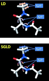
The concept of SGLD can be illustrated by Fig. 1. In normal dynamics, such as in Langevin dynamics, kinetic energy distributes evenly among all degrees of freedom, i.e., kT/2 per degree of freedom. The alanine dipeptide shown in Fig. 1 has high frequency motions like bond vibration and bond bending, and low frequency motions, such as the bond rotations about the ϕ, ψ dihedral angles. All these motions have the same kinetic energy, or temperature, T, in the canonical ensemble. The low frequency motions, the changes of the ϕ, ψ dihedral angels in this case, are the limiting steps for conformational searching. These low frequency motions can be enhanced by elevating temperatures. However, at high temperatures, all motions, most of them high frequency motions, are more energetic, which dramatically enlarge the accessible conformational space and shift major conformational distribution to otherwise unpopulated regions. In SGLD, the guiding forces enhance the low frequency motions, as defined by the local averaging time, t_L, while suppressing high frequency motions to maintain the overall temperature. In other words, the low frequency motions will gain more kinetic energy and become hotter. At the same time, the high frequency motions will lose kinetic energy and become cooler. The overall temperature remains unchanged. The enhancement in the low frequency motions will increase the transition of the backbone dihedral angles, which leads to an accelerated conformational searching. Because most of degrees of freedom are high frequent in nature, enhancing only the low frequency motions has a much smaller disturbance on the conformational distribution than enhancing all motions due to elevated temperatures.

Figure 1.

Thermal motions of an alanine dipeptide in Langevin dynamics and in self-guided Langevin dynamics simulations. Atoms are drawn as sticks. Carbon, oxygen, nitrogen, and hydrogen atoms are colored as grey, red, blue, and white, respectively. In LD, all motions have kinetic energies equivalent to a temperature of T, while in SGLD, low frequency motion gain more kinetic energy, becoming hotter, and high frequency motions lose some kinetic energy, becoming cooler. It is the low frequency motion that controls the conformational searching, therefore, SGLD achieves enhanced conformational searching ability without raising temperature.

SGLD relies on the guiding forces to enhance the low frequency motions. Under the effect of the guiding forces, SGLD has its own conformational distribution, defined as the SGLD ensemble. The partition function of the SGLD ensemble has been derived recently² which allows a conversion between the SGLD ensemble and the canonical ensemble so that canonical ensemble properties can be calculated from SGLD simulations through reweighting. Based on the SGLD partition function, we further developed the force-momentum based self-guided Langevin dynamics (SGLDfp)⁹ method, to directly sample the canonical ensemble without the need of reweighting.

Temperature-based replica exchange methods utilize elevated temperatures to accelerate conformational search.^{10, 11, 12, 13, 14} Through replica exchanging, a system can overcome energy barriers at high temperatures and maintain conformational distributions at different temperatures. For large systems, elevating temperatures causes a significant change in energy distributions, which requires a large number of replicas to achieve reasonable exchange probabilities, which in turn increases simulation cost accordingly. This size dependence is termed as not size extensive. Many efforts have been dedicated to address this difficulty for large systems.^{15, 16, 17, 18, 19, 20, 21, 22, 23, 24, 25, 26}

Because SGLD accelerates conformational searching and sampling, it can also be used for replica exchange simulations. Lee and Olson applied SGLD directly to their temperature-based replica-exchange (SGLD-ReX) simulations in their study of protein folding.²⁷ Because the SGLD partition function was not available at that time, they did not include the guiding force effects in their calculation of the exchange probabilities. Therefore, it is not surprising to observe certain deviations in their simulation results. To apply SGLD properly in replica exchange simulations, the SGLD partition function must be incorporated into the exchange probability to maintain the conformational distributions at different simulation conditions.

This work presents the replica exchanging self-guiding Langevin dynamics (RXSGLD) method. The goal of this work are as follows: (1) to describe the details of the RXSGLD method and to show how to derive the exchange probability from the SGLD partition function, (2) to examine how accurately RXSGLD samples the canonical ensemble, and (3) to evaluate the conformational searching ability of RXSGLD as compared to a temperature-based replica exchange simulation method.

THEORY AND METHODS

The RXSGLD simulation method is a combination of the replica exchange approach and the SGLD method. By incorporating the SGLD partition function into the exchange probability, RXSGLD can maintain a canonical ensemble at its base stage while achieve enhanced conformational searching and sampling. Because SGLD plays a central role in this method, we first briefly introduce the SGLD method^{1, 2, 3, 9} and its conformational distribution, followed by a detailed description of the RXSGLD method.

SGLD simulation method

For any particle, i, the equation of the self-guided motion has the following general form:

$$\begin{array}{c}\hfill {\dot{\mathbf{p}}}_i={\mathbf{f}}_i+{\mathbf{g}}_i-{\gamma }_i{\mathbf{p}}_i+{\mathbf{R}}_i,\end{array}$$ (1)

where ${\dot{\mathbf{p}}}_i$ is the time derivative of momentum and f_i is the interaction force. R_i represents a random force, which is related to the mass, m_i, the collision frequency, γ_i, and the simulation temperature, T, by the following equation:

$$\begin{array}{c}\hfill ⟨{\mathbf{R}}_i\left(0\right){\mathbf{R}}_i\left(t\right)⟩=2m_{i}kT{\gamma }_i\delta \left(t\right).\end{array}$$ (2)

Equation 1 contains a guiding force, g_i, which is calculated based on the momentum, p_i, and the low frequency momentum, ${\tilde{\mathbf{p}}}_i$,

$$\begin{array}{c}\hfill {\mathbf{g}}_i\left(t\right)={\lambda }_i{\gamma }_i\left({\tilde{\mathbf{p}}}_i\left(t\right)-\xi {\mathbf{p}}_i\left(t\right)\right).\end{array}$$ (3)

Here, λ_i is the guiding factor, which defines the strength of the guiding force. When λ_i = 0, Eq. 1 reduces to that of Langevin dynamics. The parameter, ξ, is an energy conservation factor to eliminate any net energy input from the guiding force,

$$\begin{array}{c}\hfill \sum _i{\mathbf{g}}_i·{\dot{\mathbf{r}}}_i=\sum _i{\lambda }_i{\gamma }_i{\tilde{\mathbf{p}}}_i·{\dot{\mathbf{r}}}_i-\xi \sum _i{\lambda }_i{\gamma }_i{\mathbf{p}}_i·{\dot{\mathbf{r}}}_i=0.\end{array}$$ (4)

The summation in Eq. 4 runs over all particles in a simulation system. Eq. 4 means that the guiding force will not cause energy flow between the system and its environment. Instead, the guiding force will cause energy flow between different motion modes within a simulation system. The energy conservation factor on each time step is determined from the following equation:

$$\begin{array}{c}\hfill \xi =\frac{{\sum }_i{\lambda }_i{\gamma }_i{\tilde{\mathbf{p}}}_i·{\dot{\mathbf{r}}}_i}{{\sum }_i{\lambda }_i{\gamma }_i{\mathbf{p}}_i·{\dot{\mathbf{r}}}_i}.\end{array}$$ (5)

The low frequency portion of any property, P, as denoted by a “∼” cap, $\tilde{P}$, is calculated as a local average in the following progressive way:

$$\begin{array}{c}\hfill \tilde{P}\left(t\right)=\left(1-\frac{\delta t}{t_L}\right)\tilde{P}(t-\delta t)+\frac{\delta t}{t_L}P\left(t\right).\end{array}$$ (6)

This calculation is very memory efficient and is simply done by an update with current instantaneous values. This local averaging acts like a low frequency filter that reduces high frequency components while keeps low frequency contributions.² Therefore, the results from Eq. 6 are called the low frequency properties. Correspondingly, we call $P-\tilde{P}$ the high frequency property. According to Eq. 3, the guiding force has the characteristics of the low frequency momentum. As a result, it resonates and enhances low frequency motions, which in turn, accelerates conformational searching and sampling.

The low frequency and high frequency properties defined by Eq. 6 should not be understood as a separation of properties based on the motion modes. They both contain contributions from all motion modes, but with different proportions. The low frequency properties contain more contributions from low frequency motion modes, while the high frequency properties contain more from high frequency ones. In other words, every motion mode contributes to both the low frequency and the high frequency properties, but the proportion depends on its frequency.

The effects of the guiding force on the low frequency motions and high frequency motions depend on simulation systems, simulation conditions, and many other factors, such as the coupling between motion modes. Therefore, it is difficult to characterize quantitatively the effects of the guiding forces theoretically. Nonetheless, we can evaluate the effects from SGLD simulations. To summarize, we use λ_lfand λ_hf to represent the bias effects on the low frequency and high frequency energy surfaces, and use χ_lf and χ_hf to represent the effects on the low frequency and the high frequency motions, respectively. Taken together, an SGLD ensemble has a configurational partition function of the following form:²

$$\begin{array}{c}\hfill {\Theta }_{\mathrm{SGLD}}\approx \sum \exp \left(-\frac{{\lambda }_{\mathrm{lf}}{\chi }_{\mathrm{lf}}{\tilde{E}}_{\mathrm{p}}}{kT}-\frac{{\lambda }_{\mathrm{hf}}{\chi }_{\mathrm{hf}}(E_{\mathrm{p}}-{\tilde{E}}_{\mathrm{p}})}{kT}\right).\end{array}$$ (7)

Here, the summation runs over all microscopic states. The factors, λ_lfand λ_hf, which are called the low frequency energy factor and the high frequency energy factor, respectively, are calculated as the average projections of the total forces in the direction of the interaction forces as follows:

$$\begin{array}{c}\hfill {\lambda }_{\mathrm{lf}}=\frac{⟨{\sum }_i({\tilde{\mathbf{f}}}_i+{\tilde{\mathbf{g}}}_i-{\gamma }_i{\tilde{\mathbf{p}}}_i){\tilde{\mathbf{f}}}_i⟩}{⟨{\sum }_i{\tilde{\mathbf{f}}}_i{\tilde{\mathbf{f}}}_i⟩},\end{array}$$ (8)

$$\begin{array}{c}\hfill {\lambda }_{\mathrm{hf}}=\frac{⟨{\sum }_i\left({\mathbf{f}}_i-{\tilde{\mathbf{f}}}_i+{\mathbf{g}}_i-{\tilde{\mathbf{g}}}_i-{\gamma }_i({\mathbf{p}}_i-{\tilde{\mathbf{p}}}_i)\right)({\mathbf{f}}_i-{\tilde{\mathbf{f}}}_i)⟩}{⟨{\sum }_i({\mathbf{f}}_i-{\tilde{\mathbf{f}}}_i)({\mathbf{f}}_i-{\tilde{\mathbf{f}}}_i)⟩}.\end{array}$$ (9)

The factors, χ_lf and χ_hf, which are called the low frequency collision factor and the high frequency collision factor, respectively, are calculated according to the projections of the guiding forces in the direction of the friction forces as follows:

$$\begin{array}{c}\hfill {\chi }_{\mathrm{lf}}=\frac{{\tilde{T}}_0}{\tilde{T}}=1-\frac{⟨{\sum }_i{\tilde{\mathbf{g}}}_i{\gamma }_i{\tilde{\mathbf{p}}}_i⟩}{⟨{\sum }_i{\gamma }_i^2{\tilde{\mathbf{p}}}_i{\tilde{\mathbf{p}}}_i⟩},\end{array}$$ (10)

$$\begin{array}{ccc}\hfill {\chi }_{\mathrm{hf}}& =& \frac{T-{\tilde{T}}_0}{T-\tilde{T}}=\frac{T-{\chi }_{\mathrm{lf}}\tilde{T}}{T-\tilde{T}}\hfill \\ & =& 1-\frac{⟨{\sum }_i{\gamma }_i({\mathbf{g}}_i-{\tilde{\mathbf{g}}}_i)·({\mathbf{p}}_i-{\tilde{\mathbf{p}}}_i)⟩}{⟨{\sum }_i{\gamma }_i^2({\mathbf{p}}_i-{\tilde{\mathbf{p}}}_i)·({\mathbf{p}}_i-{\tilde{\mathbf{p}}}_i)⟩}.\hfill \end{array}$$ (11)

$\tilde{T}$ is called the low frequency temperature, which is calculated from the low frequency momentum as

$$\begin{array}{c}\hfill \tilde{T}=\frac{1}{N_{\mathrm{DF}}k}⟨\sum _i\frac{{\tilde{\mathbf{p}}}_i^2}{m_i}⟩.\end{array}$$ (12)

${\tilde{T}}_0$ is the reference low frequency temperature, which corresponds to the low frequency temperature when the guiding factors, {λ_i}, are zero.

From Eqs. 8, 9, 10, 11, we can see that in a Langevin dynamics (LD) simulation, λ_lf = 1, λ_hf = 1, χ_lf = 1, and χ_hf = 1. Therefore, from Eq. 7 we have

$$\begin{array}{c}\hfill {\Theta }_{\mathrm{LD}}=\sum \exp \left(-\frac{E_{\mathrm{p}}}{kT}\right).\end{array}$$ (13)

The partition function of the canonical ensemble from an LD simulation, Θ_LD, can be related to that of an SGLD ensemble, Θ_SGLD, by the following equation:

$$\begin{array}{ccc}\hfill {\Theta }_{\mathrm{LD}}& =& \sum \exp \left(-\frac{E_{\mathrm{p}}}{kT}\right)\hfill \\ & =& \sum \exp \left(-{\lambda }_{\mathrm{lf}}{\chi }_{\mathrm{lf}}\frac{{\tilde{E}}_{\mathrm{p}}}{kT}-{\lambda }_{\mathrm{hf}}{\chi }_{\mathrm{hf}}\frac{E_{\mathrm{p}}-{\tilde{E}}_{\mathrm{p}}}{kT}\right)\hfill \\ & & \times \exp \left(\left({\lambda }_{\mathrm{lf}}{\chi }_{\mathrm{lf}}-1\right)\frac{{\tilde{E}}_{\mathrm{p}}}{kT}+\left({\lambda }_{\mathrm{hf}}{\chi }_{\mathrm{hf}}-1\right)\frac{E_{\mathrm{p}}-{\tilde{E}}_{\mathrm{p}}}{kT}\right))\hfill \\ & =& {\Theta }_{\mathrm{SGLD}}{⟨w_{\mathrm{SGLD}}⟩}_{\mathrm{SGLD}}.\hfill \end{array}$$

Here, w_SGLD is called the SGLD reweighting factor,

$$\begin{array}{c}\hfill w_{\mathrm{SGLD}}=\exp \left(\left({\lambda }_{\mathrm{lf}}{\chi }_{\mathrm{lf}}-1\right)\frac{{\tilde{E}}_{\mathrm{p}}}{kT}+\left({\lambda }_{\mathrm{hf}}{\chi }_{\mathrm{hf}}-1\right)\frac{E_{\mathrm{p}}-{\tilde{E}}_{\mathrm{p}}}{kT}\right).\end{array}$$ (14)

Any ensemble average, ⟨P⟩ _LD, can be calculated in an SGLD simulation as

$$\begin{array}{c}\hfill {⟨P⟩}_{\mathrm{LD}}=\frac{{⟨P{w}_{\mathrm{SGLD}}⟩}_{\mathrm{SGLD}}}{{⟨w_{\mathrm{SGLD}}⟩}_{\mathrm{SGLD}}}.\end{array}$$ (15)

To quantitatively describe the conformational search ability of an SGLD simulation, we define the self-guiding temperature as

$$\begin{array}{c}\hfill T_{\mathrm{SG}}=\frac{{\chi }_{\mathrm{hf}}}{{\chi }_{\mathrm{lf}}}T=\frac{\tilde{T}(T-{\tilde{T}}_0)}{{\tilde{T}}_0(T-\tilde{T})}T.\end{array}$$ (16)

The self-guiding temperature, T_SG, provides a rough measure of the conformational searching ability in the unit of temperature. An SGLD simulation with a self-guiding temperature of T_SG has conformational search ability comparable to that of a high temperature simulation at T = T_SG. In SGLD simulations, one can either set the guiding factors, {λ_i}, or set a target self-guiding temperature, $T_{\mathrm{SG}}^0$, and adjust the guiding factors, {λ_i}, so that T_SG approaches $T_{\mathrm{SG}}^0$.

Replica exchanging self-guiding Langevin dynamics simulation

A replica exchange simulation consists of a number of parallel simulations of identical systems, which are called replicas, at different simulation conditions, which are called stages. For a typical temperature based replica exchange simulation, replicas represent different conformational states, and stages represent different temperatures. A replica exchange means either two replicas exchanging their stages, or two stages exchanging their replicas. Both schemes have the same results but different exchanging information, which only affects communication efficiency and post processing procedures.

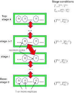
Figure 2 illustrates the basic scheme of a RXSGLD simulation. There are k+1 stages with different simulation conditions. The stage with the conditions of interest is designated as stage 0 ($T_{\mathrm{SG}}^{\left(0\right)}=T$ and T⁽⁰⁾ = T), and is called the base stage. The other k stages have different guiding temperatures, $T_{\mathrm{SG}}^{\left(i\right)}$, and the same or different temperatures, T⁽ⁱ⁾. The stage with the maximum condition is called the top stage with T^(k) and $T_{\mathrm{SG}}^{\left(k\right)}$. We use the base and top conditions to denote a replica exchange simulation, such as $T_{\mathrm{SG}}=T_{\mathrm{SG}}^{\left(0\right)}/T_{\mathrm{SG}}^{\left(k\right)}$ and T = T⁽⁰⁾/T^(k). To make all exchanges between neighboring stages to have similar acceptance ratios, it is suggested to have temperatures exponentially distributed.¹² We use the following formula to set temperatures and the self-guiding temperatures for each stage:

$$\begin{array}{c}\hfill T^{\left(i\right)}=T^{\left(0\right)}{\left(\frac{T^{\left(k\right)}}{T^{\left(0\right)}}\right)}^{\frac{i}{k}},\end{array}$$ (17a)

$$\begin{array}{c}\hfill T_{\mathrm{SG}}^{\left(i\right)}=T_{\mathrm{SG}}^{\left(0\right)}{\left(\frac{T_{\mathrm{SG}}^{\left(k\right)}}{T_{\mathrm{SG}}^{\left(0\right)}}\right)}^{\frac{i}{k}}=T^{\left(0\right)}{\left(\frac{T_{\mathrm{SG}}^{\left(k\right)}}{T^{\left(0\right)}}\right)}^{\frac{i}{k}}.\end{array}$$ (17b)

The right expression of Eq. 17b is due to the fact that $T_{SG}^{\left(0\right)}=T^{\left(0\right)}$. At different stages the temperature-based replica exchanging Langevin dynamics (TRXLD) has only different temperatures, while RXSGLD has different guiding temperatures, $\left\{T_{\mathrm{sg}}^{\left(i\right)}\right\}$, and/or different temperatures. In this work, we keep temperatures constant, T⁽ⁱ⁾ = T⁽⁰⁾, in all the RXSGLD simulations.

Figure 2.

A basic scheme describing the replica exchanging self-guided Langevin dynamics simulation. There are multiple stages with different simulation conditions, T⁽ⁱ⁾and $T_{\mathrm{SG}}^{\left(i\right)}$. The base stage has the simulation condition of interest, T⁽⁰⁾and $T_{\mathrm{SG}}^{\left(0\right)}=T^{\left(0\right)}$. A simulation system is replicated to many copies, called replicas. On each stage there are one or more replicas. Between stages, a pair of randomly chosen replicas are exchanged according to the exchanging probability. A TRXLD simulation has different stage temperatures, T⁽ⁱ⁾ ⩾ T⁽⁰⁾, but no guiding force, $T_{\mathrm{SG}}^{\left(i\right)}=T^{\left(0\right)}$, and a RXSGLD simulation has difference self-guiding temperatures, $T_{\mathrm{SG}}^{\left(i\right)}\ge T^{\left(0\right)}$.

The simulation system is replicated to many replicas. As shown in Fig. 2, one or more replicas are assigned to each stage. The number of replicas in each stage can be different. Between stages, a pair of randomly chosen replicas is exchanged according to the exchange probability, which will be described below. For simplicity, all simulations in this work use only one replica per stage.

The key quantity for a successful replica exchange simulation is the exchange probability. Based on the SGLD partition function, Eq. 7, it is straightforward to derive the exchange probability between different stages. We use ${\mathbf{X}}_m^{\left(i\right)}$ and T_m to represent conformation i and temperature of stage m. According to the SGLD partition function, Eq. 7, the distribution probability of ${\mathbf{X}}_m^{\left(i\right)}$ is

$$\begin{array}{ccc}& & {\rho }_{\mathrm{SGLD}}\left(X_m^{\left(i\right)}\right)\hfill \\ & =& \frac{1}{{\Theta }_{\mathrm{SGLD}}^{\left(m\right)}}\exp \left(-\frac{{\lambda }_{\mathrm{lf}}^{\left(\mathrm{m}\right)}{\chi }_{\mathrm{lf}}^{\left(\mathrm{m}\right)}{\tilde{E}}_{\mathrm{p}}^{\left(i\right)}}{k{T}_m}-\frac{{\lambda }_{\mathrm{hf}}^{\left(\mathrm{m}\right)}{\chi }_{\mathrm{hf}}^{\left(\mathrm{m}\right)}(E_{\mathrm{p}}^{\left(i\right)}-{\tilde{E}}_{\mathrm{p}}^{\left(i\right)})}{k{T}_m}\right)\hfill \\ & =& \frac{1}{{\Theta }_{\mathrm{SGLD}}^{\left(m\right)}}\exp \left(-{\tilde{\mu }}_{\mathrm{m}}{\tilde{E}}_{\mathrm{p}}^{\left(i\right)}-{\mu }_{\mathrm{m}}{E}_{\mathrm{p}}^{\left(i\right)}\right).\hfill \end{array}$$ (18)

Here, the parameters are defined as

$$\begin{array}{c}\hfill {\tilde{\mu }}_m=\frac{{\lambda }_{\mathrm{lf}}^{\left(m\right)}{\chi }_{\mathrm{lf}}^{\left(m\right)}-{\lambda }_{\mathrm{hf}}^{\left(m\right)}{\chi }_{\mathrm{hf}}^{\left(m\right)}}{k{T}_m}\end{array}$$ (19a)

and

$$\begin{array}{c}\hfill {\mu }_m=\frac{{\lambda }_{\mathrm{hf}}^{\left(m\right)}{\chi }_{\mathrm{hf}}^{\left(m\right)}}{k{T}_m}.\end{array}$$ (19b)

When two replicas exchange, the state of the replica system changes from {…,${\mathbf{X}}_m^{\left(i\right)}$, …,${\mathbf{X}}_n^{\left(j\right)}$, …} to {…,${\mathbf{X}}_m^{\left(j\right)}$,…, ${\mathbf{X}}_n^{\left(i\right)}$,…}, and the exchange probability, π_RX, can be expressed in the following form:

$$\begin{array}{ccc}\hfill {\pi }_{\mathrm{RX}}\left(\left\{{\mathbf{X}}_m^{\left[i\right]},{\mathbf{X}}_n^{\left[j\right]}\right\}\to \left\{{\mathbf{X}}_m^{\left[j\right]},{\mathbf{X}}_n^{\left[i\right]}\right\}\right)& =& \frac{{\rho }_{\mathrm{SGLD}}\left({\mathbf{X}}_m^{\left[j\right]}\right){\rho }_{\mathrm{SGLD}}\left({\mathbf{X}}_n^{\left[i\right]}\right)}{{\rho }_{\mathrm{SGLD}}\left({\mathbf{X}}_m^{\left[i\right]}\right){\rho }_{\mathrm{SGLD}}\left({\mathbf{X}}_n^{\left[j\right]}\right)}\hfill \\ & =& \exp (-{\tilde{\mu }}_m\left({\tilde{E}}_{\mathrm{p}}\left({\mathbf{X}}_m^{\left[j\right]}\right)-{\tilde{E}}_{\mathrm{p}}\left({\mathbf{X}}_m^{\left[i\right]}\right)\right)-{\mu }_m\left(E_{\mathrm{p}}\left({\mathbf{X}}_m^{\left[j\right]}\right)-E_{\mathrm{p}}\left({\mathbf{X}}_m^{\left[i\right]}\right)\right)-{\tilde{\mu }}_n\left({\tilde{E}}_{\mathrm{p}}\left({\mathbf{X}}_n^{\left[i\right]}\right)-{\tilde{E}}_{\mathrm{p}}\left({\mathbf{X}}_n^{\left[j\right]}\right)\right)\hfill \\ & & -{\mu }_n\left(E_{\mathrm{p}}\left({\mathbf{X}}_n^{\left[i\right]}\right)-E_{\mathrm{p}}\left({\mathbf{X}}_n^{\left[j\right]}\right)\right))\hfill \\ & \approx & \exp \left(-\left({\tilde{\mu }}_m-{\tilde{\mu }}_n\right)\left({\tilde{E}}_{\mathrm{p}}\left({\mathbf{X}}_n^{\left[j\right]}\right)-{\tilde{E}}_{\mathrm{p}}\left({\mathbf{X}}_m^{\left[i\right]}\right)\right)-\left({\mu }_m-{\mu }_n\right)\left(E_{\mathrm{p}}\left({\mathbf{X}}_n^{\left[j\right]}\right)-E_{\mathrm{p}}\left({\mathbf{X}}_m^{\left[i\right]}\right)\right)\right).\hfill \end{array}$$ (20)

Here, we approximate that the low frequency energies at different stages are the same for the same conformation: ${\tilde{E}}_{\mathrm{p}}\left({\mathbf{X}}_m^{\left[j\right]}\right)\approx {\tilde{E}}_{\mathrm{p}}\left({\mathbf{X}}_n^{\left[j\right]}\right)$, and ${\tilde{E}}_{\mathrm{p}}\left({\mathbf{X}}_n^{\left[i\right]}\right)\approx {\tilde{E}}_{\mathrm{p}}\left({\mathbf{X}}_m^{\left[i\right]}\right)$. This approximation is accurate if T_m = T_n, which is recommended for RXSGLD simulations.

For TRXLD, ${\lambda }_{\mathrm{lf}}^{\left(m\right)}=1$, ${\lambda }_{\mathrm{hf}}^{\left(m\right)}=1$, ${\chi }_{\mathrm{lf}}^{\left(m\right)}=1$, and ${\chi }_{\mathrm{hf}}^{\left(m\right)}=1$, we have ${\tilde{\mu }}_m={\tilde{\mu }}_n=0$, and ${\mu }_m={\beta }_m=\frac{1}{k{T}_m}$, ${\mu }_n={\beta }_n=\frac{1}{k{T}_n}$, and the exchange probability takes the well known form:¹²

$$\begin{array}{ccc}& & {\pi }_{\mathrm{TRXLD}}\left(\left\{{\mathbf{X}}_m^{\left[i\right]},{\mathbf{X}}_n^{\left[j\right]}\right\}\to \left\{{\mathbf{X}}_m^{\left[j\right]},{\mathbf{X}}_n^{\left[i\right]}\right\}\right)\hfill \\ & & =\exp \left(-\left({\beta }_m-{\beta }_n\right)\left(E_{\mathrm{p}}\left({\mathbf{X}}_n^{\left[j\right]}\right)-E_{\mathrm{p}}\left({\mathbf{X}}_m^{\left[i\right]}\right)\right)\right).\hfill \end{array}$$ (21)

To evaluate the exchange probability in a RXSGLD simulation, one needs the low frequency exchange coefficient, ${\tilde{\mu }}_m={\beta }_m\left({\lambda }_{\mathrm{lf}}^{\left(m\right)}{\chi }_{\mathrm{lf}}^{\left(m\right)}-{\lambda }_{\mathrm{hf}}^{\left(m\right)}{\chi }_{\mathrm{hf}}^{\left(m\right)}\right)$, and the high frequency exchange coefficient, ${\mu }_m={\beta }_m{\lambda }_{\mathrm{hf}}^{\left(m\right)}{\chi }_{\mathrm{hf}}^{\left(m\right)}$, which in turn, need parameters ${\lambda }_{\mathrm{lf}}^{\left(m\right)}$, ${\lambda }_{\mathrm{hf}}^{\left(m\right)}$, ${\chi }_{\mathrm{lf}}^{\left(m\right)}$, and ${\chi }_{\mathrm{hf}}^{\left(m\right)}$ at each stage. One way to calculate these parameters is from individual SGLD pre-simulations at all the stage conditions. A more convenient alternative is like in the SGLDfp method,⁹ to estimate these parameters during the simulations. The ensemble averages for the calculation of λ_lf, λ_hf, χ_lf, and χ_hf in Eqs. 8, 9, 10, 11 are estimated during simulations as evolving averages,

$$\begin{array}{c}\hfill \overline{\alpha }\left(t\right)=\left(1-\frac{\delta t}{t_{\mathrm{est}}}\right)\overline{\alpha }(t-\delta t)+\frac{\delta t}{t_{\mathrm{est}}}\alpha \left(t\right).\end{array}$$ (22)

Here, α(t) represents an instantaneous value of any quantity, and $\overline{\alpha }\left(t\right)$ represents its estimated average. The estimation time, t_est, is set according to the system size and estimation accuracy. Typically, we choose t_est = 10t_L.

At each exchange interval, the exchange probability between a pair of neighboring stages, ${\pi }_{\mathrm{RX}}\left(\{{\mathbf{X}}_m^{\left[i\right]},{\mathbf{X}}_{m+1}^{\left[j\right]}\}\to \{{\mathbf{X}}_m^{\left[j\right]},{\mathbf{X}}_{m+1}^{\left[i\right]}\}\right)$, is calculated according to Eq. 20 and the acceptance is determined by the Metropolis criterion: $\min \{1,{\pi }_{\mathrm{RX}}\left(\{{\mathbf{X}}_m^{\left[i\right]},{\mathbf{X}}_{m+1}^{\left[j\right]}\}\to \{{\mathbf{X}}_m^{\left[j\right]},{\mathbf{X}}_{m+1}^{\left[i\right]}\}\right)\}$. Here, m is alternately odd and even stage numbers. Once a replica exchange is accepted, the replicas at the mth and the (m+1)th stages are exchanged. Due to the differences in either the temperatures or the self-guiding temperatures, or both, the momentum, p_i, is scaled by a temperature-scaling factor,

$$\begin{array}{c}\hfill {{\mathbf{p}}^{\prime }}_i^{\left(n\right)}=s_{mn}{\mathbf{p}}_i^{\left(m\right)},\end{array}$$ (23a)

$$\begin{array}{c}\hfill {{\mathbf{p}}^{\prime }}_i^{\left(m\right)}=s_{nm}{\mathbf{p}}_i^{\left(n\right)},\end{array}$$ (23b)

$$\begin{array}{c}\hfill s_{mn}=\sqrt{\frac{T_n}{T_m}}=\frac{1}{s_{nm}}.\end{array}$$ (24)

Also, the low frequency momentum, ${\tilde{\mathbf{p}}}_i$, is scaled by a low frequency temperature-scaling factor,

$$\begin{array}{c}\hfill {\tilde{\mathbf{p}}}_i^{\prime \left(n\right)}={\tilde{s}}_{mn}{\tilde{\mathbf{p}}}_i^{\left(m\right)},\end{array}$$ (25a)

$$\begin{array}{c}\hfill {\tilde{\mathbf{p}}}_i^{\prime \left(m\right)}={\tilde{s}}_{nm}{\tilde{\mathbf{p}}}_i^{\left(n\right)},\end{array}$$ (25b)

$$\begin{array}{c}\hfill {\tilde{s}}_{mn}=\sqrt{\frac{{\tilde{T}}_n}{{\tilde{T}}_m}}=\frac{1}{{\tilde{s}}_{nm}}.\end{array}$$ (26)

Between exchanges, standard SGLD simulations are performed at all stages. The SGLD simulation details can be found elsewhere.^{1, 2}

Simulation details

The RXSGLD method has been implemented and is available in CHARMM^{28, 29} version c36 and AMBER³⁰ version 12. The simulation results reported here are obtained with CHARMM. Eight stages are used for all replica exchange simulations reported here. Exchanges are attempted every 1000 time steps. Simulation information and trajectories are output by stages separately for easy processing and analysis. All RXSGLD simulations use a local average time of 0.2 ps. All RXSGLD simulations in this work have $T_{\mathrm{SG}}^{\left(i\right)}>T_{\mathrm{SG}}^{\left(0\right)}=T^{\left(0\right)}$ and T⁽ⁱ⁾ = T⁽⁰⁾ and all TRXLD simulations have $T_{\mathrm{SG}}^{\left(i\right)}=T^{\left(0\right)}$ and T⁽ⁱ⁾ > T⁽⁰⁾, with $T_{\mathrm{SG}}^{\left(i\right)}$ and T⁽ⁱ⁾ on stage i are calculated with Eqs. 17a, 17b.

RESULTS AND DISCUSSIONS

In this section, through three example systems we examine the conformational sampling accuracy and conformational search efficiency of the RXSGLD method. There are many replica exchange methods available,^{12, 15, 16, 17, 18, 19, 21, 22, 23, 24, 25, 26, 31, 32, 33, 34, 35, 36, 37, 38, 39, 40, 41, 42, 43, 44, 45, 46, 47, 48, 49, 50, 51, 52, 53, 54, 55, 56, 57, 58, 59, 60, 61, 62, 63, 64, 65, 66, 67, 68, 69, 70, 71, 72, 73, 74, 75} it is not practical to have a thorough comparison with all the methods. In this work, we only compare RXSGLD with TRXLD to provide a general understanding of its performance.

The skewed double well system

First, we use this thoroughly studied simple system to examine the accuracy and efficiency of the RXSGLD method. A skewed double well system represents the simplest system with an energy barrier to cross. This system has only one particle, and the particle moves on a skewed double well energy surface of the following form:

$$\begin{array}{c}\hfill {\varepsilon }_{\mathrm{p}}(x,y,z)=\frac{a}{w^2}(x^2+z^2)+\frac{b}{w^4}{y}^2{(y-w)}^2+\frac{s}{w}y.\end{array}$$ (27)

The parameter, a, defines the energy surface in the x and z dimensions, and the parameters, b and w, defines a double well potential in the y dimension. There are two wells, one at y = 0 and the other at y = w. The skew parameter, s, defines the energy difference between the two wells. There are only three degrees of freedom and the partition function can be separated for each degree of freedom,

$$\begin{array}{c}\hfill {\Theta }_{\mathrm{xz}}=\frac{\pi kT{w}^2}{a},\end{array}$$ (28a)

$$\begin{array}{c}\hfill {\Theta }_{\mathrm{y}}={\int }_{-\infty }^{\infty }\exp \left(-\frac{\frac{b}{w^4}{y}^2{(w-y)}^2+\frac{s}{w}y}{kT}\right)dy.\end{array}$$ (28b)

The ensemble average properties can be calculated from the following equations:

$$\begin{array}{c}\hfill E_{xz}=kT,\end{array}$$ (29a)

$$\begin{array}{c}\hfill E_y=\frac{1}{{\Theta }_{\mathrm{y}}}{\int }_{-\infty }^{\infty }\left(\frac{b}{w^4}{y}^2{(w-y)}^2+\frac{s}{w}y\right)e^{-\frac{\frac{b}{w^4}{y}^2{(w-y)}^2+\frac{s}{w}y}{kT}}dy,\end{array}$$ (29b)

$$\begin{array}{c}\hfill {\rho }_{xz}\left(r_{xz}\right)=\frac{2a}{kT{w}^2}{e}^{-\frac{a{r}_{xz}^2}{kT{w}^2}},\end{array}$$ (30a)

$$\begin{array}{c}\hfill {\rho }_y\left(y\right)=\frac{1}{{\Theta }_{\mathrm{y}}}{e}^{-\frac{\frac{b}{w^4}{y}^2{(w-y)}^2+\frac{s}{w}y}{kT}}.\end{array}$$ (30b)

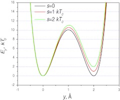
Here, $r_{xz}=\sqrt{x^2+z^2}$. In this work, we chose a = 20000kT₀, b = 160kT₀, andw = 2Å. Three double well systems with different skew parameters, s = 0, kT₀, and 2kT₀, were examined. Here, T₀ = 50 K is the base temperature. Figure 3 shows the three skewed double well potentials in the y dimension. The two wells are at y = 0 Å and y = 2 Å and have different depths depending on the skew parameter. An argon atom was simulated on the energy surfaces. 8 stages and 8 replicas were used for each replica exchange simulation. The TRXLD simulations were carried out at T = 50/100 K and the RXSGLD simulations were at T = 50 K, T_SG = 50/100 K. A collision frequency of 100/ps was used to force the motion of the argon atom into a random walk in nature. A time step of 1 fs was used and the simulation length was 100 ns for each simulation. The local averaging time was set to t_L = 0.2ps for all RXSGLD simulations.

Figure 3.

The skewed double well potentials in the y-dimension. The potential function is shown in Eq. 27. The skew parameter, s, controls the relative depths of the two wells. The energy barrier between the two wells is about 10 kT₀.

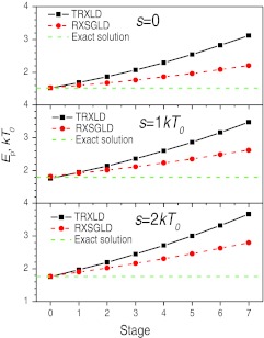
Ensemble distributions are the first thing to examine to validate a simulation method. Figure 4 compares the average energies of each stage in the TRXLD, RXSGLD, as well as the numerical solutions from Eq. 29a and Eq. 29b. As can be seen, at the base stages, both methods produce correct ensemble average energies for the three systems. The base stage averages are listed in Table 1 for a quantitative comparison. These results serve as the first evidence that RXSGLD produces correct ensemble average properties at the base stages. Comparing the average energies of all stages, we can see that RXSGLD has smaller energy differences across the stages than TRXLD, this is because SGLD only enhances the low frequency motions and has less perturbation on conformational distribution than raising temperatures.

Figure 4.

Average stage energies in the TRXLD and RXSGLD simulations. The solutions from Eq. 29a are shown as dashed lines. The TRXLD simulations has 8 stages with T = 50/100 K, and the RXSGLD simulations have 8 stages with T_SG = 50/100 K and T = T₀ = 50 K.

Table 1.

Average properties of the skewed double well systems on the base stage (T = 50 K). x₁ is the fraction of distribution in the well near y = 0 Å.

Skew parameter	Methods	Epot, kT	x1
0	solution	1.525	0.5
	TRXLD	1.513 ± 0.002	0.477 ± 0.006
	RXSGLD	1.520 ± 0.002	0.491 ± 0.006
kT	solution	1.796	0.738
	TRXLD	1.760 ± 0.010	0.763 ± 0.005
	RXSGLD	1.827 ± 0.009	0.705 ± 0.006
2kT	solution	1.762	0.878
	TRXLD	1.754 ± 0.012	0.881 ± 0.003
	RXSGLD	1.772 ± 0.011	0.876 ± 0.003

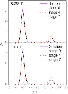
To demonstrate the different effects on conformational distributions, we plotted the distributions in the y dimension and in the x-z dimensions from the TRXLD and RXSGLD simulations in Fig. 5 and Fig. 6. From Fig. 5, we can see clearly that, at the base stages, i.e., stage 0, both simulations produced distributions that agreed well with the solution of Eq. 30b. These results further demonstrate that RXSGLD preserves canonical ensemble distributions at the base stage. At stage 4 and stage 7, the y-distributions deviate from the numerical solutions due to elevated temperatures in the TRXLD simulations or due to the guiding effects in the RXSGLD simulations. These results demonstrate that in the y dimension, where the atom has a low frequency motion, the guiding forces and raising temperatures have similar effects.

Figure 5.

The y-coordinate distributions at stage 0, 4, and 7 in the TRXLD (T = 50/100 K), RXSGLD (T_SG = 50/100 K and T = T₀ = 50 K) simulations. The data is for the skewed double well system with s = 2kT₀.

Figure 6.

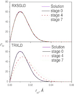
The x-z distributions at stage 0, 4, and 7 in the TRXLD (T = 50/100 K), RXSGLD (T_SG = 50/100Kand T = T₀ = 50K) simulations. The data is for the skewed double well system with s = 2kT₀.

Figure 6 shows the distributions in the x-z dimensions where the particle moves in high frequency modes. Clearly, at stage 0, both simulation results agree well with the solution of Eq. 30a. However, at other stages the distributions from TRXLD and from RXSGLD are different. The distributions at stages 4 and 7 from TRXLD deviate significantly from that at the base stage, indicating raising temperatures also change the distributions in the x-z dimensions. However, the distributions on stages 4 and 7 from the RXSGLD simulations are almost the same as on the base stages. That means the guiding forces change little in the x-z dimensions, where the atom has high frequency motions. This difference contrasts SGLD and high temperature simulations, and explains why the energy differences across the stages in RXSGLD are smaller than those in TRXLD. RXSGLD stages differ only in the low frequency motions while TRXLD stages are different in all motions.

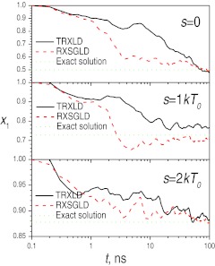
The conformational search efficiency can be examined by the convergence in the conformational distribution. We use the distribution fraction in the well near y = 0, denoted as x₁, to examine the convergence. Figure 7 shows x₁ on the base stages during the replica exchange simulations, as well as the solutions using Eqs. 30a, 30b. By the end of the simulations, all results approach the solutions fairly well (Table 1), which again demonstrates that RXSGLD can sample the conformation correctly. As can be seen from Fig. 7, the RXSGLD results approach the solutions faster than the TRXLD results for all three cases. These results prove that RXSGLD has better conformational searching efficiency than TRXLD. For this one-particle system, the improvement is not that significant. As will be seen below, differences will be more significant for larger systems.

Figure 7.

Distribution fractions of well 1, x₁, on the base stages (T₀ = 50 K) from the TRXLD (T = 50/100 K) and RXSGLD (T_SG = 50/100 K and T = T₀ = 50 K) simulations. The solutions of Eq. 30 are shown as dashed lines.

The β-hairpin folding peptide with implicit solvent

Protein folding simulation is a major application of enhanced sampling methods. Because of a large number of degrees of freedom, protein conformational space is huge, making protein folding a challenge for computational studies. Replica exchange methods have been a preferred choice for protein folding studies due to its strong conformational searching ability. Here, we chose a 9-residue β-hairpin folding peptide to examine how the RXSGLD method performs for this realistic system. This 9-residue peptide studied here was designed by Blanco et al.⁷⁶ and was modified from the β-hairpin of α-amylase inhibitor tendamistat (residues 15-23). The amino acid sequence of this peptide is: Tyr(1)-Gln(2)-Asn(3)-Pro(4)-Asp(5)-Gly(6)-Ser(7)-Gln(8)-Ala(9). The screened Coulomb potential implicit solvent model (SCPISM) was used^{77, 78} to describe the solvent effects. Using an implicit solvation model in this example allows a fairly thorough sampling of the conformational space so that we can compare the conformational distributions quantitatively.

We performed an 8-stage TRXLD simulation (T = 274/400 K) and an 8-stage RXSGLD simulation (T = 274 K, T_sg = 274/400 K). All simulations started from a fully extended conformation and were 200 ns in length. The collision frequency was set to 1/ps.

Because there are many degrees of freedom in proteins, it is often more convenient to cluster protein conformations to provide a simplified description of the conformational distribution. Here, we propose a subset indexing clustering (SIC) method as described below to cluster simulation conformations.

• (1)
  Subsets: separate the conformational variables to subsets:

  $$\begin{array}{ccc}\hfill \left\{x_1,x_2,...,x_n\right\}& =& \{\left(x_{a1},x_{a2},...\right),\left(x_{b1},x_{b2},...\right),...,\hfill \\ & & \left(x_{m1},x_{m2},...\right)\}\hfill \\ & =& \left\{s_a,s_b,...,s_m\right\}.\hfill \end{array}$$

  The conformation variables are chosen based on research interest, such as dihedral angles of amino acids, hydrogen bonds, or secondary structures.
• (2)
  Regions: define regions in the distribution of each subset variables. The distribution is generated from simulation results. For a subset, s_i, there are k_i regions: {R_i(1), R_i(2), …, R_i(k_i)}, and s_i ∈ R_i(1) + R_i(2) + ··· + R_i(k_i). The region index is defined as

  $$\begin{array}{c}\hfill I_i=\left\{\begin{array}{cc}\begin{array}{c}1\\ 2\\ \cdots \\ k_i\end{array}& \begin{array}{c}{s}_i\in R_i\left(1\right)\\ s_i\in R_i\left(2\right)\\ \cdots \\ s_i\in R_i\left(k_i\right)\end{array}\end{array}\right..\end{array}$$ (31)
• (3)Clusters: A cluster represents a unique list of the region indexes of all subsets, {I₁, I₂, …, I_m}. Total possible cluster numbers is the product of the numbers of subset regions, $N_c={\prod }_{i=1}^m{k}_i$. A conformation is identified as a SIC by indexing its subset regions,

$$\begin{array}{c}\hfill \mathrm{SIC}\left(x_1,x_2,...,x_n\right)=\{I_1,I_2,...,I_m\}.\end{array}$$

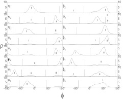
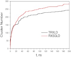
Because the SIC method does not evaluate pairwise properties between conformations, it is very efficient and its computing cost is an order of N. For proteins, it is a natural choice to choose the ϕ, ψ dihedral angles of each amino acid as a subset. The dihedral angle distribution regions for each amino acid in protein structures have been well documented and can be used for the subset index clustering of protein conformations. For this small peptide of 9-amino acids, it is more informational to use each of its 16 ϕ, ψ dihedral angles (tyr(1) does not have ϕ and Ala(9) does not have ψ) as a subset to perform the clustering. Figure 8 plots the population of the 16 dihedral angles from all stages of the replica exchange simulations. Based on the distributions, we define k_i = 1, 2, 2, 2, 2, 1, 2, 2, 2, 2, 2, 2, 3, 2, 2, 1 regions for the 16 dihedral angles, respectively. From the number of regions we can calculate that there are total 12288 possible clusters. The actual number of clusters visited by all the replicas in both the TRXLD and RXSGLD simulations is 1145, among which TRXLD visited 1056 clusters, and RXSGLD visited 730 clusters. However, at the base stage, TRXLD visited 244 clusters and RXSGLD visited 283 clusters. In other words, TRXLD searched many high temperature conformations. It is not surprising that at high temperatures, the replicas searched more conformational space. However, at high temperatures, the replicas very likely climbed into conformations that would have low probabilities at the base temperature and failed to reach the base stage. While in the RXSGLD simulation, the guiding forces accelerate conformational searching but keep the focus on the high probability region. In other words, raising temperatures increases accessible conformational space that lead to a search of low populated regions, while the guiding forces accelerate conformational search without significantly increasing the accessible conformational space so that the conformational search can be more concentrated on high population regions. We can define a conformational searching relevancy (CSR) as the number of clusters on the base stage versus those on all stages. For the TRXLD simulation, the CSR is 244/1056 = 23.1%, while for the RXSGLD simulation, the CSR is 283/730 = 38.8%. These CSR values mean that in the TRXLD simulation only 23.1% of searched conformations are of interest, while in the RXSGLD simulation, about 38.8% searched conformations are relevant.

Figure 8.

The distribution of the 16 backbone dihedral angles in the 9-reside β-hairpin folding peptide calculated from the replica exchange simulations. One to three regions are defined as labeled for each dihedral angle for the subset index clustering.

Figure 9 shows the number of clusters visited at the base stage during the TRXLD and RXSGLD simulations. Clearly, the number of clusters searched in RXSGLD increases faster than that in TRXLD, demonstrating RXSGLD has stronger conformational searching ability.

Figure 9.

Total numbers of clusters searched in the TRXLD (T = 274/500 K) and RXSGLD (T_SG = 274/400 K and T = T₀ = 274 K) simulations. The 9-residue β-hairpin folding peptide is simulated with an implicit salvation model.

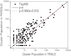
Because this β-hairpin folding peptide is a more realistic system than the double well system discussed above, it is more interesting to examine how its conformational space is sampled in RXSGLD as compared to TRXLD. Figure 10 plots the cluster populations in the RXSGLD simulation against that in the TRXLD simulation. For easy plotting in a logarithm scale, the cluster populations are counted from 1. In other words, a population of 1 means the cluster has not been visited. As can be seen from Fig. 10, the cluster population in the RXSGLD simulation correlates with that in the TRXLD simulation fairly well, even though significant fluctuation exists in those low population clusters. Figure 10 also shows a linear fit of the data (the red dashed line), which is very close to the ideal equation, y = x. This result indicates that RXSGLD can provide correct conformational sampling for this realistic peptide system.

Figure 10.

Comparison of the cluster populations between the TRXLD (T = 274/400 K) result and the RXSGLD (T_SG = 274/400 K and T = T₀ = 274 K) result. For convenience in plotting in the logarithm scale, the cluster population counts start from 1. The 9-residue β-hairpin folding peptide is simulated with an implicit salvation model. The subset indexing clustering method is described in the text.

In Fig. 10, we can see there are two high population points, which represent two major clusters. We examined the two structures and found both are hairpin-like conformations. A major difference between the two conformations is that Gly(6) changes its dihedral angle, φ₆, from region I to region II (see Fig. 8).

The β-hairpin folding peptide in aqueous solutions

A major challenge to temperature-based replica exchange simulation is its difficulties with large systems. When a system is large, the same temperature difference will cause a large energy change, which reduces the exchange probability exponentially according to Eq. 21. This phenomenon is termed as not size extensive. To achieve reasonable replica exchange probability, the number of stages and replicas, must be increased proportionally. When the number of stages is large, the diffusion of replicas from the top stage to the base stage will take a long time, which further reduces the conformational sampling efficiency.

We use an aqueous solution of this β-hairpin folding peptide to examine the application of RXSGLD to large systems. The peptide was dissolved in a box of 829 TIP3P⁷⁹ water. A sodium ion was placed in the box to neutralize the system. The box size was 30 × 30 × 30 Å.³ A collision frequency of 1/ps was used to maintain the temperature. We used the CHARMM 22 force field⁸⁰ to calculate energies and used the 3D IPS method with a local region radius of 10 Å for electrostatic and Lennard-Jones energy calculation.^{81, 82, 83} We performed three 8-stage TRXLD simulations with T = 274/310 K, 274/350 K, and 274/400 K, respectively and three 8-stage RXSGLD simulations at T = 274 K, T_SG = 274 K/310 K, 274/350 K, and 274/400 K, respectively. All simulations started from a fully extended conformation and were 20 ns in length.

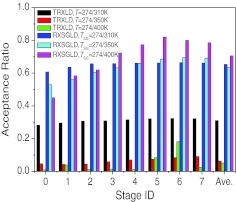
The efficiency of replica exchange simulations depends on the acceptance ratio of replica exchange. Figure 11 shows the acceptance ratios on each stage in these simulations. When the temperature range is small, T = 274/310K, the average acceptance ratio for TRXLD is 31.1%, which is acceptable. However, for more meaningful temperature ranges, T = 274/350 K and T = 274/400 K, the average acceptance ratios are 6.4% and 5.2%, which are too low. The smaller the temperature range is, the less conformational searching power a TRXLD simulation can reach. On the other hand, the lower the acceptance ratio is, the less the high temperature stages contribute to the conformational search. Therefore, to accelerate conformational searching for this large system, the number of stages must be increased to obtain a reasonable acceptance ratio and to utilize a reasonable large temperature range. In contrast to TRXLD, all three RXSGLD simulations have high acceptance ratios (65.3%, 63.5%, and 70.2%).

Figure 11.

Acceptance ratios at each stage in the TRXLD and RXSGLD simulations. The 9-residue β-hairpin folding peptide is simulated with explicit water.

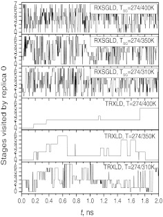
The acceptance ratios may reflect only the transition between neighboring stages. A better picture of a replica exchange simulation is the diffusion of replicas across the stages. Fig. 12 shows the stages visited by replica 0 during the simulations. For TRXLD at T = 274/310K, replica 0 took more than 0.6 ns to reach stage 7, while at T = 274/350K and T = 274/400K, replica 0 did not reach stage 7 until 2.35 ns and 3.28 ns (beyond the plotting range), respectively. While in the three RXSGLD simulations, replica 0 reached stage 7 within 0.1 ns. The fast diffusion across the stages allowed the sampling to take advantage of the maximum enhanced conformational searching at the top stage.

Figure 12.

Stage identities visited by replica 0 in the TRXLD and RXSGLD simulations. The 9-residue β-hairpin folding peptide is simulated with explicit water.

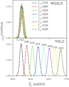
As defined by the exchange probability equations, Eqs. 20, 21, the reason for such large differences in the exchange ratios is clearly due to the difference in the energy distributions. Fig. 13 shows the potential energy distributions at different stages in the TRXLD simulation at T = 274/400 K and in the RXSGLD simulations at T_SG = 274/400 K. Clearly, in the TRXLD simulation, the energy distributions are very different from each other and there are very small overlaps between the neighboring stages, which makes exchange probability very low. In the RXSGLD simulation, the stage energy distributions are very close to each other and they overlap with each other significantly. This large overlap in stage energies makes the acceptance ratio high in RXSGLD simulations.

Figure 13.

Potential energy distributions at each stage in the TRXLD (T = 274/400 K) and RXSGLD (T_SG = 274/400 K and T = T₀ = 274 K) simulations. The 9-residue β-hairpin folding peptide is simulated with explicit water.

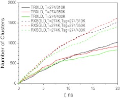
We can compare the conformational searching by examining conformational clusters searched during the simulations. Using the SIC method described above, we clustered the conformations at the base stage of the TRXLD and RXSGLD simulations. Fig. 14 compares the numbers of clusters searched in the simulations. In all RXSGLD simulations, the cluster numbers increased significantly faster than in the TRXLD simulations. These results again prove that RXSGLD has stronger conformational searching ability.

Figure 14.

The total numbers of clusters searched during the TRXLD and RXSGLD simulations. The 9-residue β-hairpin folding peptide is simulated with explicit water.

CONCLUSIONS

This work presents the replica exchanging self-guided Langevin dynamics (RXSGLD) simulation method. This method uses SGLD to enhance conformational searching and has high replica exchange efficiency. By avoiding temperature elevation, this method can be applied to large systems with high replica exchange efficiency and can use relatively few replicas to save computing cost. By incorporating the SGLD partition function into the exchanging probability, this method samples the canonical ensemble distribution at the base stage. Therefore, the RXSGLD method can be used as an alternative to the force-momentum based self-guided Langevin dynamics (SGLDfp) to directly sample canonical ensemble without the need of reweighting. Using the skewed double well systems and a β-hairpin folding peptide with implicit salvation model, we demonstrate that RXSGLD produces correct ensemble distributions while improving conformational searching and sampling. Through the β-hairpin folding simulations in explicit water, we demonstrate that RXSGLD has better size extensiveness than TRXLD.

References

- Wu X. and Brooks B. R., Chem. Phys. Lett. 381, 512 (2003). 10.1016/j.cplett.2003.10.013 [DOI] [Google Scholar]
- Wu X. and Brooks B. R., J. Chem. Phys. 134, 134108 (2011). 10.1063/1.3574397 [DOI] [PMC free article] [PubMed] [Google Scholar]
- Wu X., Damjanovic A., and Brooks B. R., “Efficient and unbiased sampling of biomolecular systems in the canonical ensemble: A review of self-guided Langevin dynamics,” in Advances in Chemical Physics, edited by Rice S. A., and Dinner A. R., (Wiley, Hoboken, 2012), Vol. 150, pp. 255. [DOI] [PMC free article] [PubMed] [Google Scholar]
- Damjanovic A., Wu X., Garcia-Moreno E. B., and Brooks B. R., Biophys. J. 95, 4091 (2008). 10.1529/biophysj.108.130906 [DOI] [PMC free article] [PubMed] [Google Scholar]
- Damjanovic A., Miller B. T., Wenaus T. J., Maksimovic P., Bertrand Garcia-Moreno E., and Brooks B. R., J. Chem. Info. Model. 48, 2021 (2008). 10.1021/ci800263c [DOI] [PubMed] [Google Scholar]
- Damjanovi A., Garcia-Moreno E. B., and Brooks B. R., Proteins: Struct., Funct., Bioinf. 76, 1007 (2009). 10.1002/prot.22439 [DOI] [PMC free article] [PubMed] [Google Scholar]
- Pendse P. Y., Brooks B. R., and Klauda J. B., J. Mol. Biol. 404, 506 (2010). 10.1016/j.jmb.2010.09.045 [DOI] [PMC free article] [PubMed] [Google Scholar]
- Lee C. I. and Chang N. Y., Biophys. Chem. 151, 86 (2010). 10.1016/j.bpc.2010.05.002 [DOI] [PubMed] [Google Scholar]
- Wu X. and Brooks B. R., J. Chem. Phys. 135, 204101 (2011). 10.1063/1.3662489 [DOI] [PMC free article] [PubMed] [Google Scholar]
- Geyer C. J. and Thompson E. A., J. Am. Stat. Assoc. 90, 909 (1995). 10.2307/2291325 [DOI] [Google Scholar]
- Swendsen R. H. and Wang J.-S., Phys. Rev. Lett. 57, 2607 (1986). 10.1103/PhysRevLett.57.2607 [DOI] [PubMed] [Google Scholar]
- Sugita Y. and Okamoto Y., Chem. Phys. Lett. 314, 141 (1999). 10.1016/S0009-2614(99)01123-9 [DOI] [Google Scholar]
- Li H., Li G., Berg B. A., and Yang W., J. Chem. Phys. 125, 144902 (2006). 10.1063/1.2354157 [DOI] [PubMed] [Google Scholar]
- Li H. and Yang W., J. Chem. Phys. 126, 114104 (2007). 10.1063/1.2710790 [DOI] [PubMed] [Google Scholar]
- Lee A. J. and Rick S. W., J. Chem. Phys. 131, 174113 (2009). 10.1063/1.3259049 [DOI] [PubMed] [Google Scholar]
- Rick S. W., J. Chem. Phys. 126, 054102 (2007). 10.1063/1.2431807 [DOI] [PubMed] [Google Scholar]
- Li X., O’Brien C. P., Collier G., Vellore N. A., Wang F., Latour R. A., Bruce D. A., and Stuart S. J., J. Chem. Phys. 127, 164116 (2007). 10.1063/1.2780152 [DOI] [PubMed] [Google Scholar]
- Li X., Latour R. A., and Stuart S. J., J. Chem. Phys. 130, 174106 (2009). 10.1063/1.3129342 [DOI] [PMC free article] [PubMed] [Google Scholar]
- Mitsutake A., Sugita Y., Okamoto Y., Faller R., Yan Q., de Pablo J. J., Fukunishi H., Watanabe O., Takada S., Calvo F., Rick S. W., Liu P., Voth G. A., Kamberaj H., van der Vaart A., Brenner P., Sweet C. R., VonHandorf D., Izaguirre J. A., Trebst S., Troyer M., and Hansmann U. H. E., J. Chem. Phys. 118, 6664 (2003). 10.1063/1.1555847 [DOI] [Google Scholar]
- Fukunishi H., Watanabe O., and Takada S., J. Chem. Phys. 116, 9058 (2002). 10.1063/1.1472510 [DOI] [Google Scholar]
- Jang S., Shin S., and Pak Y., Phys. Rev. Lett. 91, 058305 (2003). 10.1103/PhysRevLett.91.058305 [DOI] [PubMed] [Google Scholar]
- Liu P., Huang X., Zhou R., and Berne B. J., J. Phys. Chem. B 110, 19018 (2006). 10.1021/jp060365r [DOI] [PMC free article] [PubMed] [Google Scholar]
- Liu P., Kim B., Friesner R. A., and Berne B. J., Proc. Natl. Acad. Sci. U.S.A. 102, 13749 (2005). 10.1073/pnas.0506346102 [DOI] [PMC free article] [PubMed] [Google Scholar]
- Liu P. and Voth G. A., J. Chem. Phys. 126, 045106 (2007). 10.1063/1.2408415 [DOI] [PubMed] [Google Scholar]
- Ballard A. J. and Jarzynski C., Proc. Natl. Acad. Sci. U.S.A. 106, 12224 (2009). 10.1073/pnas.0900406106 [DOI] [PMC free article] [PubMed] [Google Scholar]
- Kar P., Nadler W., and Hansmann U. H., Phys. Rev. E 80, 056703 (2009). 10.1103/PhysRevE.80.056703 [DOI] [PubMed] [Google Scholar]
- Lee M. S. and Olson M. A., J. Chem. Theory Comput. 6, 2477 (2010). 10.1021/ct100062b [DOI] [PubMed] [Google Scholar]
- Brooks B. R., C. L.BrooksIII, A. D.MackerellJr., Nilsson L., Petrella R. J., Roux B., Won Y., Archontis G., Bartels C., Boresch S., Caflisch A., Caves L., Cui Q., Dinner A. R., Feig M., Fischer S., Gao J., Hodoscek M., Im W., Kuczera K., Lazaridis T., Ma J., Ovchinnikov V., Paci E., Pastor R. W., Post C. B., Pu J. Z., Schaefer M., Tidor B., Venable R. M., Woodcock H. L., Wu X., Yang W., York D. M., and Karplus M., J. Comput. Chem. 30, 1545 (2009). 10.1002/jcc.21287 [DOI] [PMC free article] [PubMed] [Google Scholar]
- Brooks B. R., Bruccoleri R. E., Olafson B. D., States D. J., Swaminathan S., Jaun B., and Karplus M., J. Comput. Chem. 4, 187 (1983). 10.1002/jcc.540040211 [DOI] [Google Scholar]
- Case D. A., Darden T. A., T. E.CheathamIII, Simmerling C. L., Wang J., Duke R., Luo R., Walker R. C., Zhang W., Merz K. M., Roberts B. P., Wang B., Hayik S., Roitberg A., Seabra G., Kolossvary I., Wu X., Brozell S., Tsui V., Gohlke H., Mongan J., Hornak V., Cui G., Beroza P., Mathews D. H., Schafmeister C., Ross W. S., and Kollman P. A., AMBER 11 (University of California, San Francisco, 2010). [Google Scholar]
- Kim J., Keyes T., and Straub J. E., J. Chem. Phys. 132, 224107 (2010). 10.1063/1.3432176 [DOI] [PMC free article] [PubMed] [Google Scholar]
- Su L. and Cukier R. I., J. Phys. Chem. B 113, 9595 (2009). 10.1021/jp900309q [DOI] [PubMed] [Google Scholar]
- Shmygelska A. and Levitt M., Proc. Natl. Acad. Sci. U.S.A. 106, 1415 (2009). 10.1073/pnas.0812510106 [DOI] [PMC free article] [PubMed] [Google Scholar]
- Mitsutake A. and Okamoto Y., Phys. Rev. E 79, 047701 (2009). 10.1103/PhysRevE.79.047701 [DOI] [PubMed] [Google Scholar]
- Mitsutake A., J. Chem. Phys. 131, 094105 (2009). 10.1063/1.3204443 [DOI] [PubMed] [Google Scholar]
- Kim J. and Straub J. E., J. Chem. Phys. 130, 144114 (2009). 10.1063/1.3108523 [DOI] [PMC free article] [PubMed] [Google Scholar]
- Kim J., Keyes T., and Straub J. E., J. Chem. Phys. 130, 124112 (2009). 10.1063/1.3095422 [DOI] [PMC free article] [PubMed] [Google Scholar]
- Kannan S. and Zacharias M., J. Struct. Biol. 166, 288 (2009). 10.1016/j.jsb.2009.02.015 [DOI] [PubMed] [Google Scholar]
- Kamberaj H. and van der Vaart A., J. Chem. Phys. 130, 074906 (2009). 10.1063/1.3077857 [DOI] [PubMed] [Google Scholar]
- Fajer M., Swift R. V., and McCammon J. A., J. Comput. Chem. 30, 1719 (2009). 10.1002/jcc.21285 [DOI] [PMC free article] [PubMed] [Google Scholar]
- Czaplewski C., Kalinowski S., Liwo A., and Scheraga H. A., J. Chem. Theory Comput. 5, 627 (2009). 10.1021/ct800397z [DOI] [PMC free article] [PubMed] [Google Scholar]
- Curuksu J. and Zacharias M., J. Chem. Phys. 130, 104110 (2009). 10.1063/1.3086832 [DOI] [PubMed] [Google Scholar]
- Chebaro Y., Dong X., Laghaei R., Derreumaux P., and Mousseau N., J. Phys. Chem. B 113, 267 (2009). 10.1021/jp805309e [DOI] [PubMed] [Google Scholar]
- Zhang J., Li W., Wang J., Qin M., and Wang W., Proteins 72, 1038 (2008). 10.1002/prot.22001 [DOI] [PubMed] [Google Scholar]
- Shen H., Czaplewski C., Liwo A., and Scheraga H. A., J. Chem. Theory Comput. 4, 1386 (2008). 10.1021/ct800063d [DOI] [PMC free article] [PubMed] [Google Scholar]
- Nadler W. and Hansmann U. H., J. Phys. Chem. B 112, 10386 (2008). 10.1021/jp805085y [DOI] [PubMed] [Google Scholar]
- Kouza M., Hu C. K., and Li M. S., J. Chem. Phys. 128, 045103 (2008). 10.1063/1.2822272 [DOI] [PubMed] [Google Scholar]
- Hritz J. and Oostenbrink C., J. Chem. Phys. 128, 144121 (2008). 10.1063/1.2888998 [DOI] [PubMed] [Google Scholar]
- Gallicchio E., Levy R. M., and Parashar M., J. Comput. Chem. 29, 788 (2008). 10.1002/jcc.20839 [DOI] [PMC free article] [PubMed] [Google Scholar]
- Fajer M., Hamelberg D., and McCammon J. A., J. Chem. Theory Comput. 4, 1565 (2008). 10.1021/ct800250m [DOI] [PMC free article] [PubMed] [Google Scholar]
- Bellesia G., Lampoudi S., and Shea J. E., Methods Mol. Biol. 474, 133 (2008). 10.1007/978-1-59745-480-3 [DOI] [PubMed] [Google Scholar]
- Athenes M. and Calvo F., ChemPhysChem 9, 2332 (2008). 10.1002/cphc.200800427 [DOI] [PubMed] [Google Scholar]
- Zhou R., Methods Mol. Biol. 350, 205 (2007). 10.1385/1-59745-189-4:205 [DOI] [PubMed] [Google Scholar]
- Zheng W., Andrec M., Gallicchio E., and Levy R. M., Proc. Natl. Acad. Sci. U.S.A. 104, 15340 (2007). 10.1073/pnas.0704418104 [DOI] [PMC free article] [PubMed] [Google Scholar]
- Thachuk C., Shmygelska A., and Hoos H. H., BMC Bioinf. 8, 342 (2007). 10.1186/1471-2105-8-342 [DOI] [PMC free article] [PubMed] [Google Scholar]
- Su L. and Cukier R. I., J. Phys. Chem. B 111, 12310 (2007). 10.1021/jp073314i [DOI] [PubMed] [Google Scholar]
- Nadler W. and Hansmann U. H., Phys. Rev. E 76, 057102 (2007). 10.1103/PhysRevE.76.057102 [DOI] [PubMed] [Google Scholar]
- Mu Y., Yang Y., and Xu W., J. Chem. Phys. 127, 084119 (2007). 10.1063/1.2772264 [DOI] [PubMed] [Google Scholar]
- Kubitzki M. B. and de Groot B. L., Biophys. J. 92, 4262 (2007). 10.1529/biophysj.106.103101 [DOI] [PMC free article] [PubMed] [Google Scholar]
- Kannan S. and Zacharias M., Proteins 66, 697 (2007). 10.1002/prot.21258 [DOI] [PubMed] [Google Scholar]
- Kamberaj H. and van der Vaart A., J. Chem. Phys. 127, 234102 (2007). 10.1063/1.2806930 [DOI] [PubMed] [Google Scholar]
- Huang X., Hagen M., Kim B., Friesner R. A., Zhou R., and Berne B. J., J. Phys. Chem. B 111, 5405 (2007). 10.1021/jp068826w [DOI] [PMC free article] [PubMed] [Google Scholar]
- Hritz J. and Oostenbrink C., J. Chem. Phys. 127, 204104 (2007). 10.1063/1.2790427 [DOI] [PubMed] [Google Scholar]
- Hagen M., Kim B., Liu P., Friesner R. A., and Berne B. J., J. Phys. Chem. B 111, 1416 (2007). 10.1021/jp064479e [DOI] [PMC free article] [PubMed] [Google Scholar]
- Brenner P., Sweet C. R., VonHandorf D., and Izaguirre J. A., J. Chem. Phys. 126, 074103 (2007). 10.1063/1.2436872 [DOI] [PubMed] [Google Scholar]
- Zuckerman D. M. and Lyman E., J. Chem. Theory Comput. 2, 12001202 (2006). 10.1021/ct0600464 [DOI] [PMC free article] [PubMed] [Google Scholar]
- Zhang W., Wu C., and Duan Y., J. Chem. Phys. 123, 154105 (2005). 10.1063/1.2056540 [DOI] [PubMed] [Google Scholar]
- Habeck M., Nilges M., and Rieping W., Phys. Rev. Lett. 94, 018105 (2005). 10.1103/PhysRevLett.94.018105 [DOI] [PubMed] [Google Scholar]
- Gallicchio E., Andrec M., Felts A. K., and Levy R. M., J. Phys. Chem. B 109, 6722 (2005). 10.1021/jp045294f [DOI] [PubMed] [Google Scholar]
- Cheng X., Cui G., Hornak V., and Simmerling C., J. Phys. Chem. B 109, 8220 (2005). 10.1021/jp045437y [DOI] [PMC free article] [PubMed] [Google Scholar]
- Mitsutake A. and Okamoto Y., J. Chem. Phys. 121, 2491 (2004). 10.1063/1.1766015 [DOI] [PubMed] [Google Scholar]
- Rhee Y. M. and Pande V. S., Biophys. J. 84, 775 (2003). 10.1016/S0006-3495(03)74897-8 [DOI] [PMC free article] [PubMed] [Google Scholar]
- Nguyen P. H., J. Chem. Phys. 132, 144109 (2010). 10.1063/1.3369626 [DOI] [PubMed] [Google Scholar]
- Itoh S. G., Okumura H., and Okamoto Y., J. Chem. Phys. 132, 134105 (2010). 10.1063/1.3372767 [DOI] [PubMed] [Google Scholar]
- Cukier R. I., J. Chem. Phys. 134, 045104 (2011). 10.1063/1.3548074 [DOI] [PubMed] [Google Scholar]
- Blanco F. J., Jimenez M. A., Herranz J., Rico M., Santoro J., and Nieto J. L., J. Am. Chem. Soc. 115, 5887 (1993). 10.1021/ja00066a092 [DOI] [Google Scholar]
- Hassan S. A. and Mehler E. L., Proteins 47, 45 (2002). 10.1002/prot.10059 [DOI] [PubMed] [Google Scholar]
- Hassan S. A., Mehler E. L., Zhang D., and Weinstein H., Proteins 51, 109 (2003). 10.1002/prot.10330 [DOI] [PubMed] [Google Scholar]
- Jorgensen W. L., Chandrasekhar J., Madura J. D., Impey R. W., and Klein M. L., J. Chem. Phys. 79, 926 (1983). 10.1063/1.445869 [DOI] [Google Scholar]
- A. D.MacKerellJr., Bashford D., Bellott M., R. L.DunbrackJr., Evanseck J. D., Field M. J., Fisher S., Gao J., Guo H., Ha S., Joseph-McCarthy D., Kuchnir L., Kuczera K., Lau F. T. K., Mattos C., Michnick S., Ngo T., Nguyen D. T., Prodhom B., W. E.ReiherIII, Roux B., Schlenkrich M., Smith J. C., Stote R., Straub J., Watanabe M., Wiorkiewicz-Kuczera J., Yin D., and Karplus M., J. Phys. Chem. B 102, 3586 (1998). 10.1021/jp973084f [DOI] [PubMed] [Google Scholar]
- Wu X. and Brooks B. R., J. Chem. Phys. 122, 44107 (2005). 10.1063/1.1836733 [DOI] [PMC free article] [PubMed] [Google Scholar]
- Wu X. and Brooks B. R., J. Chem. Phys. 129, 154115 (2008). 10.1063/1.2992601 [DOI] [PMC free article] [PubMed] [Google Scholar]
- Wu X. and Brooks B. R., J. Chem. Phys. 131, 024107 (2009). 10.1063/1.3160730 [DOI] [PMC free article] [PubMed] [Google Scholar]