The Effect of Geographical Scale of Sampling on DNA Barcoding

Abstract

Eight years after DNA barcoding was formally proposed on a large scale, CO1 sequences are rapidly accumulating from around the world. While studies to date have mostly targeted local or regional species assemblages, the recent launch of the global iBOL project (International Barcode of Life), highlights the need to understand the effects of geographical scale on Barcoding's goals. Sampling has been central in the debate on DNA Barcoding, but the effect of the geographical scale of sampling has not yet been thoroughly and explicitly tested with empirical data. Here, we present a CO1 data set of aquatic predaceous diving beetles of the tribe Agabini, sampled throughout Europe, and use it to investigate how the geographic scale of sampling affects 1) the estimated intraspecific variation of species, 2) the genetic distance to the most closely related heterospecific, 3) the ratio of intraspecific and interspecific variation, 4) the frequency of taxonomically recognized species found to be monophyletic, and 5) query identification performance based on 6 different species assignment methods. Intraspecific variation was significantly correlated with the geographical scale of sampling (R-square = 0.7), and more than half of the species with 10 or more sampled individuals (N = 29) showed higher intraspecific variation than 1% sequence divergence. In contrast, the distance to the closest heterospecific showed a significant decrease with increasing geographical scale of sampling. The average genetic distance dropped from > 7% for samples within 1 km, to < 3.5% for samples up to > 6000 km apart. Over a third of the species were not monophyletic, and the proportion increased through locally, nationally, regionally, and continentally restricted subsets of the data. The success of identifying queries decreased with increasing spatial scale of sampling; liberal methods declined from 100% to around 90%, whereas strict methods dropped to below 50% at continental scales. The proportion of query identifications considered uncertain (more than one species < 1% distance from query) escalated from zero at local, to 50% at continental scale. Finally, by resampling the most widely sampled species we show that even if samples are collected to maximize the geographical coverage, up to 70 individuals are required to sample 95% of intraspecific variation. The results show that the geographical scale of sampling has a critical impact on the global application of DNA barcoding. Scale-effects result from the relative importance of different processes determining the composition of regional species assemblages (dispersal and ecological assembly) and global clades (demography, speciation, and extinction). The incorporation of geographical information, where available, will be required to obtain identification rates at global scales equivalent to those in regional barcoding studies. Our result hence provides an impetus for both smarter barcoding tools and sprouting national barcoding initiatives—smaller geographical scales deliver higher accuracy.

“If we study a system at an inappropriate scale, we may not detect its actual dynamics and patterns but may instead identify patterns that are artifacts of scale. Because we are clever at devising explanations of what we see, we may think we understand the system when we have not even observed it correctly.”

(J.A. Wiens 1989: Spatial Scaling in Ecology. p. 390)

The vision of encyclopaedic and instant species-level knowledge at the hands of every human being is enormously attractive for the scientific and nonacademic community alike. A testimony to this in the last few years has been the tremendous increase in DNA barcoding activity, engaging thousands of researchers and at least 150 institutions in 45 countries around the globe (Stoeckle and Hebert 2008). The official launch of the international Barcode of Life (iBOL) project in late 2010 marks the beginning of a major production phase where the goal is half a million barcoded species, or more than a quarter of those described since Linnaeus, in 5 years (Vernooy et al. 2010; http://www.ibol.org). This effort is spurred by the grand goal of a complete Life-on-Earth barcode database, a resource that will answer any query of species identification, be it for a part, product or any life stage of an organism. The barcode library promises to overcome the infamous “taxonomic impediment” and democratize access to biodiversity and taxonomy (e.g., Holloway 2006; Larson 2007).

As with any new grand idea the scientific community was quick to scrutinize the feasibility and assumptions of this proposed panacea (e.g., Moritz and Cicero 2004; Will and Rubinoff 2004; Meyer and Paulay 2005; Will et al. 2005; Cameron et al. 2006; Hickerson et al. 2006; Meier et al. 2006; Elias et al. 2007; Song et al. 2008; Dasmahapatra et al. 2009; Siddall et al. 2009). In turn, the criticisms have been met with abundant case studies showing fascinating new applications (Clare et al. 2009; Cohen et al. 2009; Eaton et al. 2009; Holmes et al. 2009; Jurado-Rivera et al. 2009; Marra et al. 2009; Meiklejohn et al. 2009; Saunders 2009; Hajibabaei et al. 2011; Hrcek et al. 2011; Rougerie et al. 2011). However, one criticism in particular is fundamental to determining the likely power and accuracy of any final database used for species identification—the effect of sampling (Moritz and Cicero 2004; Meyer and Paulay 2005; Meier et al. 2006; Wiemers and Fiedler 2007; Zhang et al. 2010; Hendrich et al. 2010; Virgilio et al. 2010). Early papers demonstrating the success of barcoding identification (e.g., Hebert et al. 2003, 2004; Ball et al. 2005; Hogg and Hebert 2004; Barrett and Hebert 2005; Smith et al. 2005) generally shared: (i) very few individuals sampled per species, 2–3 on average, (ii) inclusion of a small fraction of the global species richness of the target clade, and (iii) samples came from a restricted geographical area (but see Hebert et al. 2004, based on samples from across North America). While recent studies have improved on the first condition, most are still geographically restricted and include a small proportion of the extant species belonging to the studied clade (e.g., Hebert et al. 2010; Janzen et al. 2009). Indeed, the fact that the “barcoding gap” documented in such studies is exaggerated due to poor sampling has been widely recognized (Meyer and Paulay 2005; Wiemers and Fiedler 2007). On the other hand, with improved algorithms, a barcoding gap is not necessarily a prerequisite for correct species assignment of queries (Ross et al. 2008; Lou and Golding 2010; Virgilio et al. 2010).

With the launch of the iBOL-project, the DNA barcoding enterprise is now operating at a global scale, and instead of targeting regional species assemblages, it is targeting clades. The difference is significant and can be compared with the traditional identification keys DNA Barcoding intends to automate (Janzen et al. 2009; Packer et al. 2009). A key to a regional species assemblage can be made simpler and use superior characters than that to the entire clade because many species of the clade will be missing from a particular region and can be excluded from the key. Also, part of a species' complete phenotypic variation is regularly lacking from a certain region, also facilitating the production of a diagnostic key. Similarly, genetic distances between species will be larger, and so delimitation easier, since some species of the clade are missing from the assemblage. Likewise, intraspecific variation in a given region will not represent the species total variation also facilitating DNA-based delimitation. Therefore, we expect unambiguous species-level identification to present a greater challenge for DNA Barcoding on a global level. To date, there have been limited tests of these theoretical expectations, although several clade-targeted studies have given similar hints, for example, Agrodiaetus butterflies (Wiemers and Fiedler 2007), Grammia moths (Schmidt and Sperling 2008), Protocalliphora blowflies (Whitworth et al. 2007), Agelenopsis spiders (Ayoub et al. 2005), Sigaus grasshoppers (Trewick 2008), Sternopriscus beetles (Hendrich et al. 2010), Mantellidae frogs (Vences et al. 2005), and Crocus flowers (Seberg and Petersen 2009).

Here, we test the effect of the geographical scale of sampling on species attributes affecting DNA Barcoding and on different identification methods, asking how will DNA Barcoding scale-up? We use the terms “scale effect” and “scale dependency” in the sense of Wiens (1989), that is, that “the [spatial] scale of a study may have profound effects on the patterns one finds.” Our focus is hence on changing patterns with spatial scale, although likely underlying processes will be considered in the discussion. Although a few previous empirical studies have addressed sampling (Meyer and Paulay 2005; Wiemers and Fiedler 2007), these did not investigate the effect of geographical scale explicitly. We explore the effect of scale on: (i) intraspecific genetic variation, (ii) interspecific divergence or genetic distance to the closest heterospecific, and (iii) the ratio of intraspecific variation and interspecific divergence termed the “species differentiation” and indicative of the identification success (Ross et al. 2008). In addition, we assess the degree of species monophyly for increasing geographical scales, which might not be essential for identification of samples against a reference database (it is algorithm dependent; DeSalle et al. 2005; Meier et al. 2006; Ross et al. 2008) but is certainly important if single loci are used to delimit species as reciprocally monophyletic clusters (see discussions in Sites and Marshall 2004; Hickerson et al. 2006; De Quieroz 2007; Knowles and Carstens 2007). By resampling, we estimate how the amount of intraspecific variation sampled depends on different geographical sampling strategies. Finally, we test how the geographical scale of sampling affects the identification success of queries using a range of suggested methods (see Meier et al. 2006; Ross et al. 2008).

We focus on diving beetles (family Dytiscidae), aquatic predatory insects inhabiting a range of running and standing water bodies from springs, streams and rivers to temporary rainwater pools, bogs, ponds, and lakes. The tribe Agabini comprises medium sized black or reddish brown water beetles with some 360 species distributed worldwide but most diverse in the northern hemisphere (Nilsson 2001; Ribera et al. 2003). Agabini are very uniform in morphology and color and therefore often difficult to identify, male genitalia being routinely required for correct identification (Nilsson and Holmen 1995; Foster and Bilton 1997). Three genera together containing about 100 species are known from Europe and North Africa (Nilsson 2003). Although species are superficially very similar, it is not uncommon to find 6 to 10 different species in the same habitat and locality. Taxonomically, the Agabini are well studied in the western Palaearctic region (Larson and Nilsson 1985; Fery and Nilsson 1993; Nilsson 1994; Nilsson and Holmen 1995), and although some new species are still being discovered in Europe, especially from the Mediterranean peninsula (Foster and Bilton 1997; Millán and Ribera 2001), their ease of sampling and relatively well-known taxonomy makes them an ideal group for testing the effects of geographical scale on relevant parameters for DNA Barcoding.

MATERIALS AND METHODS

Field Sampling and DNA Sequencing

Agabini beetles were collected in 96–99% ethanol with an aquatic hand net. The sampling strategy aimed to collect all species present within major running and standing water assemblages in a number of regions from North Sweden via Germany, the UK, France and Spain to Morocco in the south, and European part of Russia in the east (Fig. 1). Samples were sorted and identified to morphological species following the most recent world and Palaearctic catalogs (Nilsson 2001, 2003). Identifications were rechecked using genitalia in light of the molecular data, in particular if sister species showed a nonmonophyletic pattern. For every locality, DNA was extracted for up to 5 individuals per species. Genomic DNA was extracted from muscle tissue in the prothoracic region with Wizard SV 96-well plates according to the manufacturers' instructions (Promega, UK). An 825-bp region from the 3′ end of mitochondrial cytochrome oxidase I (CO1) was amplified with primers “Pat” and “Jerry” (Simon et al. 1994) “Ron Inosine,” “Ron Dyt,” “Pat Dyt,” and “Patty” (Isambert et al. 2011). Note that the 3′ end of CO1 is not the standardized DNA Barcoding fragment of CO1 for animals officially selected (Hanner 2009: see Roe and Sperling 2007 for relative position), but the most commonly used part in beetle systematics. Roe and Sperling (2007) found that nucleotide changes were heterogenous across the CO1-CO2 complex in a sliding window approach but no difference in the overlap between intraspecific and interspecific variation when comparing the 2 commonly used CO1 fragments (LCO-HCO vs. Pat-Jerry). In fact, they found the optimal 600-bp window to lie in between and overlapping with both. We therefore feel confident that the results would be comparable independent of which of the 2 fragments are used. If anything, the fragment used here would be a more consistent divergence estimate due to its longer fragment length, which was why Roe and Sterling proposed a lengthening of the DNA Barcoding fragment into the “Pat-Jerry” part. Amplification conditions used with Bioline Taq were 94° for 2 min, 35 to 40 cycles of 94° for 30 s, 53° for 60 s and 70° for 120 s, and a final extension of 70° for 10 min. PCR products were cleaned with a 96-well Millipore multiscreen plate, sequenced in both directions using a Big Dye 3.1 terminator reaction, and analyzed on an ABI 3730 automated sequencer. Only primers Jerry as forward, and either PatDyt or Patty as reverse, were used as sequencing primers. Contigs were assembled and edited in Sequencher 4.5. Sequences are deposited in GenBank under accession codes JQ355008–JQ356531.

FIGURE 1.

Geographical distribution of sampled localities including NCBI GenBank records.

Sequences were aligned with clustal X version 2 (Larkin et al. 2007). The alignment was cropped to a 734-bp matrix and 103 sequences lacking more than 25.6% of this region were excluded from further analysis. An additional 115 sequences of CO1 from Agabini beetles originating in Europe (including the Canary Islands and Madeira) Morocco, and Iran were also downloaded from NCBI GenBank, origin determined with latitude and longitude coordinates from the original publications and included in the analyses.

Data Analyses

Analyses of genetic and geographic distances were carried out in R statistical software (http://www.r-project.org) using the Ape library (Paradis et al. 2004). Genetic distances and neighbor-joining trees were calculated using the Kimura 2-parameter model (Kimura 1980), implemented in the Barcode of Life Data System (Ratnasingham and Hebert 2007). To test if the estimated proportion of nonmonophyletic species was algorithm dependent, we also ran parsimony analyses using TNT ver. 1.0 (Goloboff et al. 2008) and Bayesian analysis using MrBayes 3.2 (Ronquist et al. 2012) on the full data set. For the parsimony analysis, we used heuristic search strategies developed for large data sets (Goloboff 1999), in particular a “driven search” approach until minimum length was hit 10 times by means of a combination of sectorial searches and tree fusing, each under default settings in TNT. For the Bayesian analysis, we used one of the most parsimonious trees as a starting tree for the MCMC chain to shorten run time (see Hunt et al. 2007). One million generations was sampled every 1000th generation in each of 2 separate runs with 4 chains (1 cold and 3 incrementally heated). A partitioned GTR +I+G model was specified for each of the codon positions. Partitions were given separate rate multipliers and parameters were unlinked across partitions except branch lengths and topology. Prior and proposal settings were left as default. Convergence was monitored with the PSRF and average deviation of split frequency statistics. Results were summarized with a majority-rule consensus after a burn-in fraction of 25% had been removed. Intraspecific and interspecific distances were calculated using taxonomic species as units. The possible effects of cryptic diversity are addressed in the Results and Discussion. We estimated the age of divergence between 14 sister species pairs based on an uncorrelated relaxed lognormal molecular clock applied to a species level matrix of the CO1 data set using BEAST v. 1.5.4 (Drummond and Rambaut 2007). Since interspecific coalescence events in the gene tree must be older than the time at which gene flow between the incipient species ceased (Wakeley 2000; Degnan and Rosenberg 2009), the gene tree can be used as a conservative age estimate of how young recent sister species pairs are. The mean of the lognormal clock rate was set to 3.54% divergence per million years after the recent calibration of CO1 for a group of beetles (Papadopoulou et al. 2010). This should be more accurate for CO1 data sets than the generally used 2–2.3% insect mitochondrial clock (Brower 1994), which is partly based on more slowly evolving ribosomal genes. The standard deviation (SD) of the clock rate was given an uninformative prior (0 to infinity) thus allowing for the deviation from a strict clock to be estimated. To derive the posterior probability distribution of the sister species divergence dates, we gave them uniform priors bound between 0 and 1 billion years. An unlinked GTR+I+G substitution model was used with separate rates for each codon position. Two independent MCMC analyses each ran for 50 million generations with parameters sampled every 2000 generations. A burn-in of 20% was removed from each run before combining the samples. Tracer (Rambaut and Drummond 2007) was used to check for convergence of the chain and effective sample sizes of parameters.

With the estimated ages of closely related sister-species pairs, we categorized the probability of reciprocal monophyly following the work of Rosenberg (2003) and the simulation study by Hudson and Coyne (2002). The calculations are based on the assumptions of treating the 2 species as 2 separate panmictic populations with a constant population size of 10⁶ since the split of a panmictic ancestral population. The estimations are further calculated for a maternally inherited, selectively neutral and nonrecombining, mitochondrial marker, as we assume is the case for CO1. The life cycle is univoltine with one generation per year. Hudson and Coyne (2002: their Table 1) give waiting times for probabilities 0.05, 0.5, and 0.95 of reciprocal monophyly for a mitochondrial marker whereas Rosenberg's (2003: his Table 1) equivalent waiting times need to be halved for a maternally inherited marker with an effective population size of 0.5 Ne.

TABLE 1.

Studied Agabini species with number of individuals per species, geographical extent of sampled individuals in kilometers, maximum intraspecific variation and distance to closest heterospecific (Kimura 2-parameter)

Species	Individuals	Kilometers	Intra, K2P	Inter, K2P
Agabus affinis	35	2148	0.0117	0.0000
Agabus alexandrae	4	230	0.0000	0.0490
Agabus amoenus	1	0	NA	0.1019
Agabus arcticus	15	1858	0.0341	0.0277
Agabus aubei	3	27	0.0055	0.0785
Agabus biguttatus	47	3034	0.0499	0.0348
Agabus biguttulus	1	0	NA	0.0000
Agabus binotatus	4	68	0.0000	0.0034
Agabus bipustulatus	419	6135	0.0318	0.0000
Agabus brunneus	52	1677	0.0056	0.0000
Agabus cephalotes	5	0	0.0000	0.0382
Agabus clypealis	2	0	0.0000	0.0102
Agabus congener	17	2276	0.0102	0.0000
Agabus conspersus	10	230	0.0100	0.0603
Agabus didymus	92	2887	0.0116	0.0973
Agabus dilatatus	1	0	NA	0.0207
Agabus elongatus	1	0	NA	0.0865
Agabus faldermanni	1	0	NA	0.0492
Agabus fulvaster	2	159	0.0027	0.0137
Agabus fuscipennis	2	2073	0.0096	0.0567
Agabus glacialis	1	0	NA	0.0000
Agabus guttatus	55	2650	0.0654	0.0000
Agabus heydeni	11	937	0.0056	0.0277
Agabus labiatus	55	3256	0.0313	0.0000
Agabus lapponicus	13	3187	0.0211	0.0000
Agabus lineatus	3	153	0.0046	0.0171
Agabus maderensis	1	0	NA	0.0568
Agabus melanarius	7	2010	0.0027	0.0676
Agabus nebulosus	65	2492	0.0110	0.0453
Agabus nevadensis	2	1	0.0000	0.0000
Agabus paludosus	41	4070	0.0343	0.0636
Agabus psuedoclypealis	5	0	0.0017	0.0102
Agabus ramblae	1	0	NA	0.0000
Agabus rufulus	1	0	NA	0.0068
Agabus serricornis	4	78	0.0034	0.0746
Agabus sturmii	123	3393	0.0107	0.0277
Agabus uliginosus	1	0	NA	0.0171
Agabus undulatus	28	2974	0.0120	0.0783
Agabus unguicularis	9	3231	0.0113	0.0746
Agabus wollastoni	3	10	0.0018	0.0206
Agabus zimmermanni	3	0	0.0027	0.0000
Ilybius aenescens	19	1878	0.0032	0.0685
Ilybius albarracinensis	6	0	0.0056	0.0102
Ilybius angustior	4	264	0.0014	0.0000
Ilybius ater	24	2245	0.0057	0.0867
Ilybius chalconatus	30	4881	0.0297	0.0000
Ilybius cinctus	2	0	0.0000	0.1384
Ilybius crassus	5	103	0.0043	0.0867
Ilybius dettneri	6	306	0.0000	0.1031
Ilybius erichsoni	7	85	0.0062	0.0604
Ilybius fenestratus	27	2212	0.0082	0.0822
Ilybius fuliginosus	81	3451	0.0186	0.0000
Ilybius guttiger	42	1897	0.0061	0.0034
Ilybius hozgargantae	1	0	NA	0.1031
Ilybius meridionalis	25	1418	0.0130	0.0000
Ilybius montanus	32	1686	0.0189	0.0000
Ilybius neglectus	12	1502	0.0035	0.0000
Ilybius opacus	1	0	NA	0.0000
Ilybius picipes	7	469	0.0000	0.0000
Ilybius quadriguttatus	45	3061	0.0208	0.0034
Ilybius satunini	26	155	0.0071	0.0000
Ilybius similis	2	41	0.0000	0.1139
Ilybius subaeneus	35	3450	0.0298	0.0906
Ilybius subtilis	1	0	NA	0.0604
Ilybius wasastjernae	5	759	0.0123	0.0000
Ilybius vittiger	1	0	NA	0.1384
Platambus lunulatus	1	0	NA	0.0723
Platambus maculatus	46	2809	0.0132	0.0723
Mean	24	1234	0.0115	0.0384

Resampling

The most widely sampled species, Agabus bipustulatus, was represented by 419 individuals in our data set, sampled throughout Europe. It is also a species whose phylogeography has been extensively investigated by Drotz (2003) and Drotz et al. (2001, 2010), and all CO1 sequences from these studies were downloaded from GenBank. Assuming that this combined data set covers the full genetic variation of the species, this provides us with an opportunity to test how many individuals need to be sampled in order to sample all the genetic variation of a taxon, and what is the most cost effective way of sampling. To examine this, the A. bipustulatus data set was resampled according to 3 main strategies; (i) “Random sampling,” (ii) “Local sampling,” where additional samples are taken as geographically close as possible to any previous sample, and (iii) “Maximum distance sampling” where additional samples are taken as geographically distant as possible from an original random starting point. This last approach was conducted in 2 ways. First, by maximizing the geographical distance between each additional sample and the geographically closest previous sample and secondly, by maximizing the sum of geographical distances to all previous samples. Thirty different sample sizes between 2 and 350 were repeated 100 times for each of the 4 sampling strategies. This analysis was also repeated on all species with more than 55 individuals in the entire data set: Agabus labiatus, A. nebulosus, A. sturmii, A. didymus, and Ilybius fuliginosus. In each case, we recorded the sample size at which 95% of the total genetic variation in the complete sample was recovered, a measure of the sample size needed to estimate genetic variation.

Test of Identification

To test the effect of the geographical scale of sampling on identification success, we defined multiple local, national, and regional subsets of the entire continental data set. Each sequence from each data set was used as a query against the remaining data set using different identification criteria. For distance-based methods, we used the “best match,” “best close match,” and “all species barcode” method of Meier et al. (2006; also used by Virgilio et al. 2010) as well as the clustering threshold (1%) approach of Meier et al. (2006; their Table 5) using TaxonDNA/SpeciesIdentifier 1.7.7 software tool (Meier et al. 2006). Under Best match, the query is identified by the reference sequence with the smallest genetic distance to the query and for a correct identification no heterospecific sequence(s) must have an equally small distance. Best close match adds a threshold condition for the closest match to be granted identification privileges. Under all species barcode, all conspecific reference sequences have a smaller genetic distance to the query than any heterospecific sequence for identification. The clustering method clusters sequences into profiles in which all sequences are less than a threshold value from at least one other sequence in the profile but can be more than the threshold value from other sequences in the profile (Meier et al. 2006). The query was considered correctly identified if grouped in a profile of only conspecific sequences. We also calculated for each geographic range category the proportion of nonmonophyletic species and implemented 2 tree-based identification methods for queries differing in their sensibility to nonmonophyly of species. Our strict tree-based method (called “tree-based identification sensu Hebert” by Meier et al.) requires the query to cluster with all conspecific barcodes in a monospecific clade (i.e., requiring monophyly of species). Our liberal tree-based method follows Ross et al. (2008) and considers a query to be successfully identified if nested within, or sister to, a mono- and conspecific clade but does not require species monophyly. Singletons were not used as queries (but were part of the reference data sets) in order to not confound the effect of spatial scale with the issue of singletons and when the correct species is not present in the reference data set. Singletons anyhow represent only a small fraction of the data set (< 1%) and would have a minor effect. We used 1% as a threshold in accordance with the official identification engine at BOLD (http://www.boldsystems.org), for the best close match and “clustering threshold” distance methods. Tree-based methods used NJ (ties broken randomly) and a K2P model as described above. For each method, we recorded the proportion of correctly identified queries. To get a relevant measure of uncertainty, independent of whether the identification was correct or not, we calculated the proportion of queries with more than one reference species within the threshold value of 1%. Basically, the best close match together with this ambiguity measure, both at a threshold of 1%, imitates the algorithm and presentation of identification results by the official BOLD identification engine (Ratnasingham and Hebert 2007).

RESULTS

DNA was extracted from 2082 individuals, of which 1524 individuals (73%) were successfully sequenced for CO1 with a high-throughput protocol. The sample represented 52 different taxonomic species, which gives an average of 29 sequences per species. The number of individuals per species varied from 1 up to 419 in the commonly occurring A. bipustulatus, dispersed throughout Europe (Table 1). GenBank sequences added another 16 species not previously represented in the matrix and together the 68 species represent about 70% of the known Agabini fauna of West Palearctic.

Intraspecific Genetic Variation

Maximum intraspecific distances were found in Agabus guttatus (6.5%) and Agabus biguttatus (5.0%). These 2 species are part of a taxonomically difficult species complex with very little character variation (the guttatus-group sensu Foster and Bilton 1997) that remains in need of revision. For example, Agabus nitidus (Fabricius 1801), a synonym of A. biguttatus in recent catalogs (Nilsson 2001, 2003) is sometimes treated as a separate species (e.g., Sanchez-Fernandez et al. 2004). Our COI data for both species contain 3 distinct haplotype clusters, which may represent cryptic species, and we therefore report values both treating each as a single species (T1) and as 3 candidate species (T2).

Mean intraspecific variation across all species with multiple sequences were: T1: 1.04%, (N = 53), T2: 0.83%, (N =57) which increased to T1: 1.63%, (N =29), T2: 1.28%, (N =31) for species with > 10 individuals and to T1: 2.12%, (N=17), T2: 1.58%, (N =17) for species with > 30 individuals. Twenty species or 35–38% (T1-T2) had intraspecific variation of > 1%. Linear regressions of maximum intraspecific distance as a function of the number of sampled individuals were significant (T1: P =0.0295, T2: P=0.00327) but had a low explanatory power (T1: Adjusted R-square = 0.0717, T2: 0.131), and the intraspecific variation was much more strongly dependent on the geographical extent of sampled individuals (T1: Adjusted R-square =0.384, P=4.49× 10⁻⁷, T2: 0.626, P =1.46× 10⁻¹³, Fig. 2a,b). Note that treating A. guttatus and A. biguttatus as a single species results in the 2 outliers in the upper part of Figure 2a and that a much better fit (R² =0.63 vs. 0.38) is observed when they are treated as multiple taxa (Fig. 2b).

FIGURE 2.

Maximum intraspecific variation (K2P) against maximum geographic extent (km) of sampled individuals. (a) Agabus guttatus and Agabus biguttatus treated as one species each (linear regression, $Y=5.25\times 10^{-6}x+2.05\times 10^{-3}$, Adjusted R-square =0.384, P<0.001). (b) Outliers A. guttatus and A. biguttatus each subdivided into 3 species candidates (linear regression $Y=4.45\times 10^{-6}x+1.52\times 10^{-3}$, Adjusted R-square =0.626, P <0.001).

Interspecific Genetic Divergence

Minimum interspecific divergence ranged from 0 to 14%. Thirty species, or 44% (T1, T2: 31 species or 43%), had less than 1% divergence from the closest heterospecific sequence. Intra- and interspecific distances overlapped substantially (Fig. 3a,b). The effect of the geographical scale of sampling on the distance to the closest heterospecific was investigated by creating 5 geographical distance categories < 1, < 10, < 100, < 1000, and < 10000 km. For each distance category, all interspecific genetic distances were calculated and the minimum recorded for each species. Genetic distance to the closest heterospecific declined from an average of 7.08% to 3.45%, as the geographic range of sampling was increased from < 1 to < 10000 km (Fig. 4). Geographical distance categories differ significantly in the minimum genetic divergence between species (analysis of variance, F = 20, degrees of freedom =1.256, P <0.01).

FIGURE 3.

Histogram of maximum intraspecific variation (black) and minimum interspecific divergence (grey) for complete data set. (a) Agabus guttatus and A. biguttatus treated as one species each. (b) A. guttatus and A. biguttatus each subdivided into 3 species candidates. Note that closest interspecific divergence is recorded for each species so that sister species divergences are recorded twice in the frequency distribution.

FIGURE 4.

The effect of geographic scale of sampling on the closest interspecific divergence. Minimum interspecific divergences across species in 5 distance categories. In each category, all interspecific distances between individuals with a pairwise geographical distance of less than the category value was calculated and the minimum was recorded for each species. Genetic distance is significantly smaller in the 10 000 km category compared with 1, 10, and 100 km category (one-way ANOVA, Tukey HSD, P <0.01).

Intraspecific Variation/Interspecific Divergence

The combined scale effect of the above can be measured as species differentiation sensu Ross et al. (2008)—that is, the ratio between intra- and interspecific distances (Fig. 5). This ratio more than doubles from 0.11 for the smallest geographic distance category to 0.26 for the highest (Fig. 5a). This predominantly results from rapid declines in the distance to the closest heterospecific as more closely related taxa are encountered in the geographically expanding data set (Fig. 5b).

FIGURE 5.

The effect of geographic scale of sampling on the intraspecific × interspecific interaction. (a) Relationship between log geographic distance categories and the species differentiation, that is, the ratio between intraspecific variation and interspecific divergence. (b) Interspecific and intraspecific distances across 5 geographical distance categories separated by species. Each line represents a different species. gray = minimum interspecific distance, black = maximum intraspecific distance.

Species Monophyly

The data set was subdivided into a set of geographically restricted data sets representing local, national, regional, and finally continental scales (Table 2). The proportion of nonmonophyletic species in each data set was recorded with a neighbor-joining tree under a K2P model. The number of nonmonophyletic species increased drastically as the geographic extent of sampling increased (Fig. 6). At local and national levels 5% and 13%, respectively, of species showed para- or polyphyletic patterns. However, at 3 regional levels representing North Europe (including Great Britain), Central Europe and Southwest Europe (including North Morocco), 22% of species showed para- or polyphyletic patterns. In the complete European data set, 19 of 53 multiply sampled species, or 36%, were nonmonophyletic (Supplementary Fig. 1, doi: 10.5061/dryad.2rg92p5v). A similar but slightly higher proportion of nonmonophyletic species were derived from the parsimony analysis (Supplementary Fig. 2: 40%, 21 of 53, estimated from the strict consensus of 43 MPT at length 2459) as well as with Bayesian analysis (Supplementary Fig. 3: 38%, 20 of 53, estimated from the majority-rule consensus of 2 × 750 sampled trees).

TABLE 2.

Data sets of increasing geographic inclusiveness and the effect on species monophyly

Area	Individualsa	Sppb	Spp > 1 Indc	N-M Sppd	Prop N-M Sppe	Prop N-M, Spp. > 1 Indf
Local
1 Albacete	61	9	8	0	0	0
2 Alentejo—Algarve	83	3	3	0	0	0
3 Ávila—Cáceres—Toledo	55	6	6	0	0	0
4 Azrou Talass	18	6	3	0	0	0
5 Bavaria	95	13	12	0	0	0
6 Beira Alta	75	11	9	1	0.0909	0.1111
7 Brandenburg—Mecklenburg	27	9	5	0	0	0
8 Carrick—Cumbria	276	13	13	0	0	0
9 Cataluña	54	6	6	0	0	0
10 Cornwall	88	10	8	0	0	0
11 Corse	23	6	5	0	0	0
12 French Alps	41	9	7	0	0	0
13 Hebrides	65	7	6	0	0	0
14 Latvia	39	14	8	1	0.0714	0.125
15 Norfolk	78	13	10	2	0.1538	0.2
16 Öland—Småland	121	19	15	0	0	0
17 Västerbotten—Ångermanland	127	27	17	3	0.1111	0.1765
18 Viana do Castelo	34	6	5	1	0.1667	0.2
19 Volgograd—Astrachan	141	19	15	2	0.1053	0.1333
Mean	79	10.8	8.47	0.53	0.0368	0.0498
National
France (11, 12)	65	14	11	0	0	0
Germany (5, 7)	123	15	12	1	0.0667	0.0833
Portugal (2, 6, 18)	197	14	13	2	0.1429	0.1538
Spain (1, 3, 9)	187	15	11	3	0.2000	0.2727
Sweden (16, 17)	294	36	30	6	0.1667	0.2000
UK (8, 10, 13, 15)	514	23	21	2	0.0870	0.0952
Mean	230	19.5	16.33	2.33	0.1105	0.1342
Regional
C Europe	228	27	22	2	0.0741	0.0909
N Europe	851	41	34	9	0.2195	0.2647
SW Europe—Morocco	409	21	17	5	0.2381	0.2941
Mean	496	29.7	24.33	5.33	0.1772	0.2166
Continental
Europe ( + Morocco, Iran)	1638	68	53	19	0.2794	0.3585

^aInds, number of individuals in each data set.

^bSpp, number of species.

^cSpp > 1 Ind, number of species with multiple individuals.

^dN-M Spp, number of nonmonophyletic species.

^eProp N-M Spp, proportion of nonmonophyletic species.

^fProp N-M Spp > 1 Ind, proportion of nonmonophyletic species, calculated only for species with multiple individuals.

FIGURE 6.

The effect of geographical scale of sampling on species monophyly. Categories equal: local (N= 19), national (N = 6), regional (N = 3), continental (N =1) see Table 2. Species with a single representative was not included in the total when calculating the proportion since they could not be nonmonophyletic.

Dating and Tests of Lineage Sorting

We inferred a gene tree of CO1 with a relaxed molecular clock and estimated the posterior probability distribution of divergence times for 14 recent sister species pairs using a molecular clock rate (Fig. 7). The SD of the clock rate indicated that the data depart significantly from a strict molecular clock (SD =0.36, 95% highest posterior density [HPD] =0.19–0.52). The used mean rate of 0.0177 substitutions per site per million year used as a calibration with an uninformative prior on the SD resulted in a 95% HPD clock rate interval of 0.0162–0.0192 substitutions per site per million year. Mean divergence age between sister species pairs ranged from 0.099 to 1.16 Ma, with the highest upper bound of the 95% HPD at 2.02 Ma (Table 3). Based on these age estimates, we categorized the pairs into probability classes of reciprocal monophyly (Table 3). None of the 14 sister species pairs or triplets had a probability of being reciprocally monophyletic > 0.95. Nine of the 14 pairs had a probability of being reciprocally monophyletic < 0.5 even when using the upper bound of the 95% HPD. Six of the pairs had a probability of < 0.05 of being reciprocally monophyletic, if calculated with the estimated mean ages. In addition, 2 of the recent sister species pairs that were monophyletic but included few sampled individuals are predicted to become nonmonophyletic with more sampling, as the probability of reciprocal monophyly for these were < 0.5 (< 0.05 with mean age) (Table 3). A low probability of reciprocal monophyly indicates that the nonmonophyly is likely due to incomplete lineage sorting.

FIGURE 7.

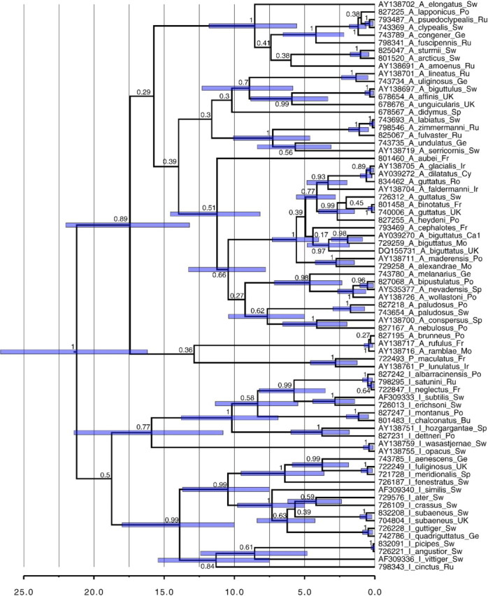
Calibrated gene tree with a single representative terminal per species using a lognormal relaxed clock. Scale is in millions of years. Node values are posterior probability clade support. Bars represent the 95% HPD interval around the dated nodes (only for nodes >0.5 in posterior probability).

TABLE 3.

Closely related sister species pairs or triplets and probability of reciprocal monophyly

Sister species pair	RMa	Mean age	95% HPDb	Probability RM
Ilybius fuliginosus—I. meridionalis	No	0.53	0.18–0.97	< 0.5 ( < 0.95)
Ilybius quadriguttatus—I. guttiger	No	0.47	0.15–0.87	< 0.5 ( < 0.5)
Ilybius angustior—I. picipes	No	0.099	0.0026–0.25	< 0.05 ( < 0.05)
Ilybius opacus—I. wasastjernae	No	0.42	0.11–0.80	< 0.5 ( < 0.5)
Ilybius montanus—I. chalconatus	No	1.16	0.44–2.02	< 0.95 ( < 0.95)
I. neglectus—I. satunini	No	0.33	0.055–0.66	< 0.05 ( < 0.5)
Agabus brunneus—A. ramblae—A. rufulus	No	0.42	0.14–0.76	< 0.5 ( < 0.5)
Agabus affinis—A. biguttulus	No	0.35	0.078–0.70	< 0.05 ( < 0.5)
Agabus bipustulatus—A. nevadensis	No	0.56	0.10–1.21	< 0.5 ( < 0.95)
Agabus congener—A. lapponicus	No	1.03	0.38–1.71	< 0.95 ( < 0.95)
Agabus labiatus—A. zimmermanni	No	0.16	0.011–0.37	< 0.05 ( < 0.05)
Agabus guttatus1—A. glacialis—A. dilatatus	No	0.60	0.23–1.04	< 0.5 ( < 0.95)
Agabus guttatus2—A. binotatus	Yes	0.22	0.031–0.48	< 0.05 ( < 0.5)
Agabus clypealis—A. pseudoclypealis	Yes	0.37	0.11–0.70	< 0.05 ( < 0.5)

Note: Estimated mean age in million years, 95% highest posterior density interval around the estimated age, and probability of reciprocal monophyly at Ne = 10⁶, given a number of assumptions (see Materials and Methods); first probability given the mean age, probability in parenthesis given the upper bound of the 95% HPD.

^aRM, reciprocal monophyly.

^bHPD, highest posterior density.

Sampling Strategies

In A. bipustulatus, with random sampling, the median of 100 resampling iterations reached 95% of the complete genetic variation after 250 individuals (Fig. 8a). The best sampling strategy to capture genetic variation in the species was to maximize the geographic distance between the new sample and the closest previous sample. With this strategy, 95% of the genetic variation was recovered with 70 individuals (Fig. 8a). The generality of this pattern was tested with all species sampled for more than 55 individuals (Fig. 8b–f). Although it may be unlikely that our samples of these species represent their total genetic variation, it is clear that any sampling strategy is highly unlikely to adequately represent the intraspecific variation with sample sizes of < 20 individuals.

FIGURE 8.

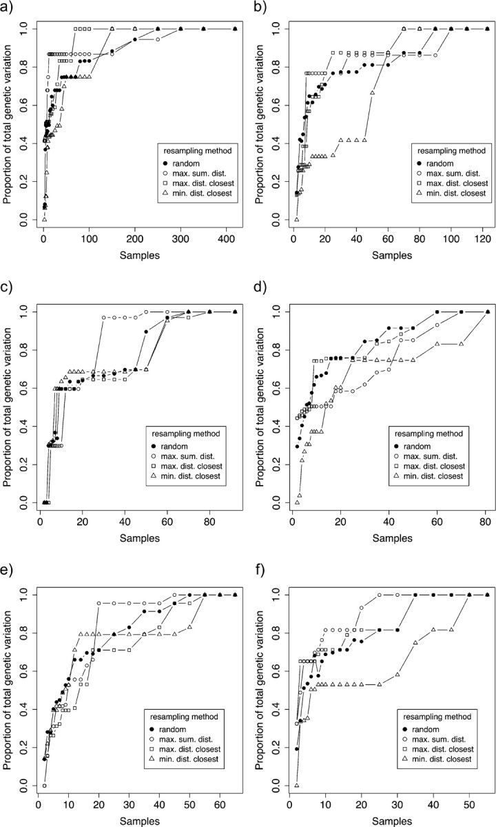
Proportion of total intraspecific genetic variation as a function of sample size. (a) Agabus bipustulatus, (b) A. sturmii, (c) A. didymus, (d) Ilybius fuliginosus, (e) A. nebulosus, (f) A. labiatus. Each data point is the median of 100 randomizations. Solid circle = random, open circle = maximum sum of geographic distances, square = maximum distance to closest geographical neighbor, triangle = minimum distance to closest geographical neighbor.

Identification of Queries

All methods showed a decline in identification success with increasing geographical scale of the reference data set (Fig. 9a; Appendix A1). The distance-based best match and best closest match decreased form a median value of 100% correct species assignments in 19 local data sets, to 91% in the continental data set. There was no significant difference between BM and BCM because singletons were not used as queries in the test. The stricter all species barcode and clustering threshold method decreased more radically from 95% to 100% at local scale, 84–91% at national scale, 81% at regional scale, and 44–45% at continental scale (Fig. 9a). The liberal tree-based method showed a similar behavior to BM and BCM with a smaller reduction from 100% of correct species identification on local scale to 87% on continental scale. Finally, the strict tree-based method showed a decline similar to ASB and CT from 100% on local scale to 44% on continental. The independent measure of uncertainty or ambiguity to the identifications was also highly scale dependent (Fig. 9b). Ambiguity, measured as the percentage of queries with more than one reference species within the 1% threshold, increased from a median value of null at local scales via 16% at national and regional scales to 50% at continental scale (Fig. 9b).

FIGURE 9.

The effect of spatial scale on query identification success and ambiguity. (a) proportion of correctly identified queries using 6 different methods and given as the median value for each range category. Range category: local (N = 19), national (N =6), regional (N =3), continental (N =1). Methods: BM, Best match; BCM, best close match; ASB, all species barcode; CT, clustering threshold; TBS, tree based strict; TBL, tree based liberal. (b) Proportion of ambiguous query identifications defined as more than one reference species matching the query within the 1% threshold.

DISCUSSION

The most common metrics reported in DNA barcoding studies are intraspecific genetic variation, interspecific genetic divergence to congenerics (mean or smallest, see Meier et al. 2008), and the proportion of monophyletic species or related measures on identifiable, diagnosable, or delimitable species. We have shown that all 3 metrics significantly correlate with the geographical scale of sampling, that is, are scale dependent (Figs. 2–6). The dependency of intraspecific genetic variation on geographical scale of sampling is to be expected based on widely recognized theory and concepts such as distance decay (Nekola and White 1999) and isolation by distance (Wright 1943), as well as from phylogeographic studies (Avise 2000). As a general rule, a species sampled throughout its geographical range will reveal greater genetic variation than if the variation was estimated from a single smaller region. Nevertheless, several DNA barcoding studies have reported that genetic and geographical distance was uncorrelated (Hebert et al. 2004, 2010), although these were either based on smaller geographical scales than included here or concerned more dispersive organisms such as birds. That intraspecific variation is scale dependent is not fatal for global DNA barcoding initiatives, since a representative reference library will deliver close hits to a query independent of geographical origin. However, such scale dependency does question whether effective identification can be achieved from whichever geographic region with few barcodes per species and without wide geographical coverage (Hebert et al. 2010).

So how extensive would sampling need to be to cover most of the existing intraspecific variation of a species? Agabus bipustulatus, a very widespread and extensively studied species in Europe (Drotz et al. 2001, 2010; Drotz 2003) provided an opportunity to test this question by resampling. The empirical resampling exercise gave very similar results to a recent simulation study that asked the same question (Zhang et al. 2010). With a sampling strategy where the geographical location of additional samples is randomized, a sample size of 150 would still on average retrieve less than 90% of the total variation. Zhang et al. (2010) likewise found from their simulations that if at least 95% of the genetic variation were to be discovered, a sample size of 156–1985 would be necessary. Slightly more encouraging was the sampling strategy that maximizes the geographical spread of additional samples (Fig. 7). Here, we found that 70 samples would on average retrieve the full genetic variation. The coinciding results from empirical data and simulations offer a note of caution for barcoding studies. For example, the iBOL project target is 5 million barcodes from 500 k species, that is, 10 individuals per species—far below the level at which the majority of the variation is sampled (this study; Zhang et al. 2010). What is an acceptable error rate and at what sample sizes this is generally achieved remain to be clarified: the choice of identification algorithm will also play an important role (Ross et al. 2008; Austerlitz et al. 2009; Virgilio et al. 2010). The good news is that sampling of intraspecific variation will constantly improve with the addition of barcodes.

What might be more of a problem is the decrease of genetic divergence to closest heterospecific with increased geographical scale of sampling (Fig. 4). This effect has been discussed in theory before (e.g., Meyer and Paulay 2005) but not previously quantified with empirical data. However, this effect also comes as no surprise since allopatric speciation is thought to be the most common mode of divergence (Barraclough and Vogler 2000; Coyne and Orr 2004), whereas the frequency of sympatric speciation is controversial (Fitzpatrick and Turelli 2006). If allopatric speciation is most common then we expect a species' closest relative not to co-occur in the same area but to enter a data set as the geographical scale of sampling expands. In fact Kisel and Barraclough (2010) found that geographical scale was significantly correlated with the probability of in situ island speciation across a wide range of groups from mammals, birds and lizards to flowering plants, butterflies, moths, and snails. This directly predicts that the pattern we found, of decreasing interspecific divergence with increased scale of sampling, is general, and not taxon specific.

The combined scale effect leads to a decrease in species differentiation, that is, the ratio between intraspecific variation and interspecific divergence to closest heterospecific. The fact that the 2 measures overlap broadly (Fig. 3) and that a barcoding gap does not exist (see also Meyer and Paulay 2005; Wiemers and Fiedler 2007) is not a major concern as the degree of overlap is a poor predictor of identification success (Ross et al. 2008). However, the degree of species differentiation is a better predictor and moreover at low levels of differentiation the sampling becomes crucial (Ross et al. 2008). The scale effect found therefore confirms our expectations that as DNA barcoding goes global, species identification becomes more of a challenge.

Finally, we find a highly significant effect of geographical extent of the data set and the proportion of monophyletic species. This reconciles the apparent contradiction between early DNA barcoding studies and the phylogeography literature (Funk and Omland 2003). In 19 locally restricted data sets, the mean proportion of nonmonophyletic species was less than 5%, similar to many early barcoding studies showing monophyly of > 95%. These numbers seemed to conflict with theory on speciation and lineage sorting time (Hudson and Coyne 2002; Rosenberg 2003; Hickerson et al. 2006), the abundance of Pleistocene speciation (e.g., Ribera and Vogler 2004) and not least animal mitochondrial DNA studies in which 23% of all species studied were nonmonophyletic (Funk and Omland 2003). In our complete European data set, 36% of multiply sampled species were nonmonophyletic. The tribe Agabini is distributed through the whole Holarctic, and although most lineages are geographically restricted (Ribera et al. 2003) some of the closest relatives of European species have Asian or North American distributions. The number of nonmonophyletic species in our study could therefore even be an underestimation, especially in some groups with wide distributions (e.g., the Ilybius angustior complex, Nilsson and Ribera 2007; or the subgenus Agabus (Acatodes), Ribera et al. 2003).

Even though the species attributes here shown to be significantly affected by spatial scale, have been central in the DNA Barcoding debate, the effects cannot be directly translated to identification performance since the response may be method dependent (Meier et al. 2006; Ross et al. 2008; Virgilio et al. 2010). We found however that all tested methods had a decreasing success of query identification but fell in 2 quite distinct groups. The most severely affected methods here labeled the “strict group” plummeted to less than 50% correct query identifications as spatial scale increased from local to continental and this group included all species barcode, “cluster threshold” and “strict tree-based” method. The second group we label the “liberal group” of methods and include the best match, best close match, and “liberal tree-based” method. With the less stringent requirements to assign a unique species name to a query, these methods only declined to between 87% and 91% of correct assignment at the continental scale from 100% at local scale. The results are in close agreement with the study by Virgilio et al. (2010) that compared the performance of DNA Barcoding across 6 insect orders and 4 identification criteria. They also found the all species barcode and a strict tree-based method to be outperformed by best match and best close match methods and, importantly, that identification success decreased significantly with an increase in the reference database size (in their case not directly linked to spatial scale but to the number of included species). Likewise, Ross et al. (2008) found a different version of the strict tree-based method to be conservative with lower rate of correct identification relative to distance and BLAST-based methods. On the other hand, the strict tree-based method was the only method relatively immune to making false positive identifications when the query species was not represented in the reference database. Ross et al. (2008) therefore proposed that the strict tree-based method was suitable to use during the build-up phase of a reference library, with the less conservative methods appropriate and more efficient once the genetic variation of the clade had been well sampled and characterized.

The most relevant method in practice, due to the implementation in the official BOLD identification engine, is the best close match genetic distance approach combined with an ambiguity measure (http://www.boldsystems.org: Ratnasingham and Hebert 2007). BOLD uses 1% as threshold value and determines the query as the ID of the closest match, conditional on that it is < 1% in genetic distance from the query, but if more than one species have a distance of < 1% then all species are listed (Ratnasingham and Hebert 2007). The latter is basically a warning of uncertainty or ambiguity—a single species may still have the closest match and deliver a correct identification but with several species within 1% distance to the query, the certainty of the identification is reduced. We found that the proportion of queries which will give similar warnings of uncertainty increase substantially with the geographical scale of sampling. At local scale, the average reference data set will give 100% unequivocal identifications of queries without uncertainty warnings. At continental scales, half of all query identifications will come with the uncertainty warning that multiple species match the query at < 1% (Fig. 10). So while a number of DNA Barcoding applications might find a 90% correct-and-unique species identification rate acceptable, the 50% uncertainty tagalong rate might not be. Note, however, that were we to link an online faunistic database, say Fauna Europaea (http://www.faunaeur.org), to the barcode identification engine, we could in a single step reduce this uncertainty to almost half (27%) by simply collecting the information that A. nevadensis only occurs in Spain. This would prevent all A. bipustulatus sequences from the rest of Europe from being unidentified or identified with a warning flag of uncertainty. Such “smart barcoding tools” combining genetic and distributional data is likely one way forward to cope with spatial scale effects, although for a few applications, like invasive species control, geographically restricted searches are not an option.

FIGURE 10.

Schematic representation of relative importance of processes as spatial (and temporal) scale increases, and the effect on DNA barcoding parameters as found from this study. Note that the linear slopes are simplifications and that nature of the scale effects can be noncontinuous and chaotic across different domains of scale (e.g., see Wiens 1989). The small red and yellow graphs in the figure are originally from Meyer and Paulay (2005).

An exhaustive evaluation of all suggested methods to date was beyond the scope of the present study hence the effect of spatial scale on Bayesian (Nielsen and Matz 2006; Munch et al. 2008a, 2008b), artificial intelligence (Zhang et al. 2008), decision theoretic (Abdo and Golding 2007), or other approaches to species assignment were not investigated. Neither did we test different threshold values the calculation of which has seen various proposals (e.g., Hebert et al. 2003, 2004) but used the threshold of 1% following the official identification engine of BOLD (Ratnasingham and Hebert 2007). As seen by the similar behavior of the best match (no threshold) and best close match (threshold) method (Fig. 9a), a threshold is most relevant if the reference data sets may lack the species represented by the query, which was not the case in our test where singletons were excluded as queries. The treatment of singletons is otherwise of significant importance when evaluating methods (Lim et al. 2012; see Ross et al. 2008, for an evaluation of the effect of singletons in Meier et al.'s 2006, data), since a global reference database is predicted to be lacking many species for a long time to come.

The effects of scale on DNA barcoding mirror those on local and regional diversity patterns in ecology, where it has been identified that different processes operate at different scales (Ricklefs and Schluter 1993), and that understanding from local scales is rarely enough to explain patterns at larger scales (Wiens 1989). The genetic structure of local and regional assemblages is mainly governed by contemporary ecological processes responsible for which species coexist and how closely related they are (Webb et al. 2002). If closely related species share similar ecological traits, then competitive exclusion will tend to lead to phylogenetic overdispersion, whereas environmental filtering will lead to phylogenetic clustering. Empirical community data have revealed both phylogenetic overdispersion and clustering and more importantly that the outcome itself is highly scale dependent (Kembel and Hubbell 2006; Swenson et al. 2006, 2007). In contrast, the processes involved in shaping the genetic structure of global clades are historical, namely the relative rates of past speciation, extinction, and demographic changes. The degree to which in situ speciation is a factor for regional assemblages depends on the size and location of the region. In Ontario (Hebert et al. 2003), for example, or the Area de Conservación Guanacaste (Janzen et al. 2009) in situ speciation plays a minor role, since these regions either encompass a biota assembled from recent Pleistocene recolonists or are part of a much larger ecological mosaic, respectively. In contrast, in endemic hotspot regions like Madagascar, Australia or Melanesia, in situ speciation is highly significant (e.g., Monaghan et al. 2006; Hendrich et al. 2010; Isambert et al. 2011). The key point here is that the relative importance of processes responsible for the patterns we observe (e.g., the genetic variation in DNA barcoding data sets) change with scale. As we increase the spatial scale, historical processes increase and ecological processes decrease in importance (Fig. 10). This is not in conflict with the notion that ecological determinants, like habitat permanence in the case of aquatic beetles, can drive microevolutionary adaptations (e.g., dispersal capacity) with likely implications for clade evolution (Ribera and Vogler 2000)—speciation can certainly be ecologically driven (Schluter 2000, 2001).

Of course one possible reason for nonmonophyly, or mismatch between molecular and morphological data, is that nonmonophyletic species might in fact be synonyms of the same species (Funk and Omland 2003; Meyer and Paulay 2005) and that the taxonomy of the group is in need of revision and an iterative reexamination of specimens (Hendrich et al. 2010). Many such cases have, and thanks to molecular tools, will continue to be discovered, meaning that it is worthwhile to examine our focal taxa in this light. While the majority of the cases of nonmonophyly reported here comprise taxa whose status has not previously been questioned, the status of some of the species pairs in Table 3 has indeed been challenged in the past. One of these is the A. congener–A. lapponicus pair, which due to previous doubts was investigated with quantitative morphometrics (Nilsson 1987) as well as with allozymes (Nilsson et al. 1988). Quantitative analyses of the apical shape of the male penis showed that there was a bimodal rather than continuous distribution, upheld even when the 2 taxa occurred in sympatry (Nilsson 1987; see also Foster 1992), and allozymes supported the recognition of 2 gene pools and hence 2 species (Nilsson et al. 1988). A second much doubted case is the status of A. nevadensis, restricted to the Sierra Nevada mountains in Spain, in relation to the very common, variable and widespread A. bipustulatus with which Ribera et al. (1998) suggested A. nevadensis might be synonymous. However, recent allozyme studies of the complex supports the hypothesis of reproductive isolation between the species (Drotz et al. 2010), even though A. nevadensis is deeply nested within A. bipustulatus based on CO1 (this study; Drotz et al. 2010). The species of the Agabus brunneus group (A. brunneus, A. ramblae, and A. rufulus) have only been recognized as distinct in recent years (Millán and Ribera 2001), although their status is now generally accepted, and they have been shown to differ markedly in thermal physiology (Calosi et al. 2008). The status of the Russian Ilybius satunini in relation to I. neglectus remains to be tested as it has not been treated in any modern revision. We are not aware of doubts about the remaining species pairs, although there may be cryptic taxa present in some groups; chromosome variation suggesting multiple species has been found within what is currently considered as I. montanus (Aradottir and Angus 2004) and our COI data suggest that the A. guttatus group might be hiding more species than presently recognized.

A question that remains is whether incomplete lineage sorting (see Funk and Omland 2003) is a reasonable explanation for the majority of nonmonophyletic species in this study. The probability of reciprocal monophyly of incipient species is high (> 0.9) only after they have been isolated for 2–4 times the effective population size X generations (Hudson and Coyne 2002; Rosenberg 2003; Hickerson et al. 2006). In our conservative age estimates of the 14 youngest sister species pairs among European Agabini, only one had a confidence interval that exceeded 2 million generations, the remaining 13 were younger (Table 3). This is in agreement with a study that found most Iberian endemic diving beetles to be of Pleistocene origin (Ribera and Vogler 2004). Our calculations are based on a number of assumptions and an arbitrary, but most likely too low (i.e., conservative), effective population size. We used an effective population size of 10⁶ and it is likely that for most species this should be significantly higher and conclusions even more robust. Dehling et al. (2010) estimated the available lentic (standing) and lotic (running) water habitats in Europe to 300 000 km of lake perimeter and 2 million kilometer of river length. For a widespread European species, a population size of 10⁶ hence translates to a density of 1 individual per 300 m of shore for a lentic species or 1 individual per 2 km of river for a lotic species, most certainly an underestimate. Even for species with a more limited European distribution, for example, 1/5th of the total surface, and more demanding habitat requirements, for example, 9/10th considered unsuitable for other reasons (size of water body, PH, vegetation, nutrition, substrate etc.) densities remain low (1/6 m, 1/40 m, respectively). Juliano and Lawton (1990) estimated the population density of diving beetles to an average of 5.5 individuals per species and square meter at one site in England, although this concerned Hydroporus, species with smaller body size and higher densities than Agabini. Perhaps the most unrealistic assumption is treating species as single panmictic populations. On the other hand, subdivided populations would overestimate the divergence time (Wakeley 2000) as well as increase the effective population size according to island models (Nei and Takahata 1993; but see Whitlock and Barton 1997 for alternative models). This again would argue that our estimates are conservative and conclusions realistic. Incomplete lineage sorting is therefore the preferred default explanation for the observed nonmonophyly of many species, although introgressive hybridization cannot be excluded in all cases (Funk and Omland 2003). Future studies could test these alternative hypotheses by adding nuclear loci, test for Wolbachia infection (Whitworth et al. 2007) and detailed geographic analyses of haplotype distribution in relation to species range overlap.

CONCLUSIONS

DNA barcoding is becoming an indispensable tool for species discovery and specimen identification alike. However, understanding the limits and scalability of the technique is a prerequisite not only for its usage but to predict the deliverables of DNA barcoding as a global enterprise. We have investigated the effect of increasing the geographical scale of sampling on species attributes relevant for DNA barcoding performance and on actual query identification. That the intraspecific variation increases with the geographical scale of sampling was expected as a result of isolation by distance and phylogeographic structure. Previously less realized is the significant decrease in interspecific divergence with increasing geographical scale of sampling due to encountering more closely related, allopatrically distributed, species in a geographically expanding data set. This also had the effect of increasing the proportion of nonmonophyletic species with spatial scale directly relevant for identification and delimitation methods assuming species monophyly. The efficacy of methods for query identification declined with increasing spatial scale but strict methods were more severely affected than liberal methods. However, the uncertainty of identifications showed a steep increase with geographical scale. Linking the global barcode database with faunistic/floristic online databases will therefore improve accuracy through geographically restricted query searches when the geographical origin of the query is known. We anticipate the development of various “smart” barcoding tools in this direction. For applications lacking a geographical context for specimens, limits of the precision with which specimens can be identified will differ from those estimated in local or regional contexts. The degree of scale effects will certainly vary between organism groups (their vagility and speciation history) and areas (geological and climate change history). In addition, some very useful applications of DNA Barcoding are by necessity of global character and cannot be geographically restricted, like the detection of invasive species or border control/global trade of illegal organism products. We also acknowledge that for many applications of DNA Barcoding such as life-stage association and environmental monitoring of nonstandard groups, identification to a pair, or small group of, closely related species can still be of great value and a methodological improvement. Nevertheless, the scale dependency gives an extra incentive for regional and national barcoding initiatives striving for maximal identification precision.

SUPPLEMENTARY MATERIAL

Supplementary material, including data files and/or online-only appendices, can be found in the Dryad data repository (doi: 10.5061/dryad.2rg92p5v).

FUNDING

This work was supported by the Natural Environment Research Council (NERC), UK (Grant No: NE/C510908/1).

Appendix

TABLE A1.

Proportion of correctly identified queries by 6 different methods, and a measure of identification ambiguity, for data sets of increasing geographic scale

Area	BMa	BCMb	ASBc	CTd	TBSe	TBLf	AMBg
Local
1 Albacete	1	0.983	0.983	1	1	1	0
2 Alentejo—Algarve	1	1	1	1	1	1	0
3 Ávila—Cáceres—Toledo	1	1	0.964	1	1	1	0
4 Azrou Talass	1	1	0.867	1	1	1	0
5 Bavaria	1	1	0.883	1	1	1	0
6 Beira Alta	1	1	0.945	0.959	0.959	0.959	0.041
7 Brandenburg—Mecklenburg	1	1	0.913	1	1	1	0
8 Carrick—Cumbria	1	0.989	0.989	1	1	1	0
9 Cataluña	1	1	1	1	1	1	0
10 Cornwall	1	1	0.977	1	1	1	0
11 Corse	1	1	1	1	1	1	0
12 French Alps	1	0.974	0.974	1	1	1	0
13 Hebrides	1	1	0.969	1	1	1	0
14 Latvia	0.970	0.970	0.788	0.818	0.879	0.970	0.121
15 Norfolk	0.827	0.827	0.760	0.813	0.813	0.867	0.187
16 Öland—Småland	1	0.991	0.821	0.752	1	1	0.085
17 Västerbotten—Ångermanland	0.983	0.983	0.889	0.838	0.812	0.957	0.162
18 Viana do Castelo	0.970	0.970	0.909	0.879	0.879	0.970	0.121
19 Volgograd—Astrachan	0.985	0.971	0.635	0.693	0.693	0.788	0.299
Median	1	1	0.945	1	1	1	0
National
France (11, 12)	1	0.984	0.984	0.839	1	1	0.161
Germany (5, 7)	1	1	0.908	0.833	0.925	1	0.167
Portugal (2, 6, 18)	0.995	0.995	0.964	0.954	0.954	0.990	0.046
Spain (1, 3, 9)	0.989	0.978	0.694	0.694	0.699	0.978	0.224
Sweden (16, 17)	0.951	0.951	0.764	0.691	0.764	0.924	0.267
UK (8, 10, 13, 15)	0.953	0.951	0.906	0.949	0.949	0.957	0.051
Median	0.992	0.981	0.907	0.836	0.937	0.984	0.164
Regional
C Europe	1	0.996	0.843	0.865	0.857	1	0.135
N Europe	0.954	0.954	0.810	0.812	0.842	0.947	0.159
SW Europe—Morocco	0.985	0.983	0.622	0.528	0.528	0.970	0.383
Median	0.985	0.983	0.810	0.812	0.842	0.970	0.159
Continental
Europe ( + Morocco, Iran)	0.915	0.907	0.451	0.436	0.435	0.872	0.501

^aBM, best match

^bBCM, best close match

^cASB, all species barcode

^dCT, clustering threshold

^eTBS, tree-based strict

^fTBL, tree-based liberal

^gAMB, ambiguous identifications

References

- Abdo Z, Golding B. A step toward barcoding life: a model-based, decision-theoretic method to assign genes to preexisting species groups. Syst. Biol. 2007;56:44–56. doi: 10.1080/10635150601167005. [DOI] [PubMed] [Google Scholar]
- Aradottir GI, Angus RB. A chromosomal analysis of some water beetle species recently transferred from Agabus Leach to Ilybius Erichson, with particular reference to the variation in chromosome number shown by I. montanus Stephens (Coleoptera: Dytiscidae) Hereditas. 2004;140:185–192. doi: 10.1111/j.1601-5223.2004.01837.x. [DOI] [PMC free article] [PubMed] [Google Scholar]
- Austerlitz F, David O, Schaeffer B, Bleakley K, Olteanu M, Leblois R, Veuille M, Laredo C. DNA barcode analysis: a comparison of phylogenetic and statistical classification methods. BMC Bioinformatics. 2009 doi: 10.1186/1471-2105-10-S14-S10. 10 (Suppl 14:S10) doi: 10.1186/1471-2105-10-S14-S10. [DOI] [PMC free article] [PubMed] [Google Scholar]
- Avise JC. Cambridge (MA): Harvard University Press; 2000. Phylogeography: the history and formation of species; p. 447. [Google Scholar]
- Ayoub NA, Riechert SE, Small RL. Speciation history of the North American funnel web spiders, Agelenopsis (Araneae: Agelenidae): phylogenetic inferences at the population–species interface. Mol. Phylogenet. Evol. 2005;36:42–57. doi: 10.1016/j.ympev.2005.03.017. [DOI] [PubMed] [Google Scholar]
- Ball SL, Hebert PDN, Burian SK, Webb JM. Biological identifications of mayflies (Ephemeroptera) using DNA barcodes. J. N. Am. Benth. Soc. 2005;24:508–524. [Google Scholar]
- Barraclough TG, Vogler AP. Detecting the geographical pattern of speciation from species-level phylogenies. Am. Nat. 2000;155:419–434. doi: 10.1086/303332. [DOI] [PubMed] [Google Scholar]
- Barrett RDH, Hebert PDN. Identifying spiders through DNA barcodes. Can. J. Zool. 2005;83:481–491. [Google Scholar]
- Brower AVZ. Rapid morphological radiation and convergence among races of the butterfly Heliconius erato inferred from patterns of mitochondrial DNA evolution. 1994 doi: 10.1073/pnas.91.14.6491. Proc. Natl. Acad. Sci. U.S.A. 91:6491–6495. [DOI] [PMC free article] [PubMed] [Google Scholar]
- Calosi P, Bilton DT, Spicer JI, Atfield A. Thermal tolerance and geographic range size in the Agabus brunneus group of European diving beetles (Coleoptera: Dytiscidae) J. Biogeogr. 2008;35:295–305. [Google Scholar]
- Cameron S, Rubinhoff D, Will KW. Who will actually use DNA barcoding and what will it cost? Syst. Biol. 2006;55:844–847. doi: 10.1080/10635150600960079. [DOI] [PubMed] [Google Scholar]
- Clare EL, Fraser EE, Braid HE, Fenton MB, Hebert PDN. Species on the menu of a generalist predator, the eastern red bat (Lasiurus borealis): using a molecular approach to detect arthropod prey. Mol. Ecol. 2009;18:2532–2542. doi: 10.1111/j.1365-294X.2009.04184.x. [DOI] [PubMed] [Google Scholar]
- Cohen NJ, Deeds JR, Wong ES, Hanner R, Yancy HF, White KD, Thompson TM, Wahl M, Pham TD, Guichard FM, Huh I. Public health response to puffer fish (tetrodotoxin) poisoning from mislabelled product. J. Food Prot. 2009;72:810–817. doi: 10.4315/0362-028x-72.4.810. [DOI] [PubMed] [Google Scholar]
- Coyne JA, Orr HA. Sunderland (MA): Sinauer Associates; 2004. Speciation; pp. 1–545. [Google Scholar]
- Dasmahapatra KK, Elias M, Hill RI, Hoffman JI, Mallet J. Mitochondrial DNA barcoding detects some species that are real, and some that are not. Mol. Ecol. Resour. 2009 doi: 10.1111/j.1755-0998.2009.02763.x. doi: 10.1111/j.1755–0998.2009.02763.x. [DOI] [PubMed] [Google Scholar]
- Degnan JH, Rosenberg NA. Gene tree discordance, phylogenetic inference and the multispecies coalescent. Trends Ecol. Evol. 2009;24:332–340. doi: 10.1016/j.tree.2009.01.009. [DOI] [PubMed] [Google Scholar]
- Dehling DM, Hof C, Brändle M, Brandl B. Habitat availability does not explain the species richness patterns of European lentic and lotic freshwater animals. J. Biogeogr. 2010;37:1919–1926. [Google Scholar]
- De Quieroz K. Species concepts and species delimitation. Syst. Biol. 2007;56:879–886. doi: 10.1080/10635150701701083. [DOI] [PubMed] [Google Scholar]
- DeSalle R, Egan MG, Siddall M. The unholy trinity: taxonomy, species delimitation and DNA barcoding. Philos. Trans. R. Soc. [Biol] 2005;360:1905–1916. doi: 10.1098/rstb.2005.1722. [DOI] [PMC free article] [PubMed] [Google Scholar]
- Drotz MK. Speciation and mitochondrial DNA diversification of the diving beetles Agabus bipustulatus and A. wollastoni (Coleoptera, Dytiscidae) within Macaronesia. Biol. J. Linn. Soc. 2003;79:653–666. [Google Scholar]
- Drotz MK, Brodin T, Nilsson AN. Multiple origins of elytral reticulation modifications in the West Palearctic Agabus bipustulatus complex (Coleoptera, Dytiscidae) PLoS ONE. 2010;5(2):e9034. doi: 10.1371/journal.pone.0009034. [DOI] [PMC free article] [PubMed] [Google Scholar]
- Drotz MK, Saura A, Nilsson AN. The species delimitation problem applied to the. Agabus bipustulatus complex (Coleoptera, Dytiscidae) in north Scandinavia. Biol. J. Linn. Soc. 2001;73:11–22. [Google Scholar]
- Drummond AJ, Ho SYW, Phillips MJ, Rambaut A. Relaxed phylogenetics and dating with confidence. PLoS Biol. 2006;4(5):e88. doi: 10.1371/journal.pbio.0040088. [DOI] [PMC free article] [PubMed] [Google Scholar]
- Drummond AJ, Rambaut A. “BEAST: Bayesian evolutionary analysis by sampling trees”. BMC Evol. Biol. 2007;7:214. doi: 10.1186/1471-2148-7-214. doi: 10.1186/1471-2148-7-214. [DOI] [PMC free article] [PubMed] [Google Scholar]
- Eaton MJ, Meyers GL, Kolokotronis S-O, Leslie MS, Martin MP, Amato G. Barcoding bushmeat: molecular identification of Central African and South American harvested vertebrates. Conserv. Genet. 2009;11:1389–1404. [Google Scholar]
- Elias M, Hill RI, Willmott KR, Dasmahapatra KK, Brower AVZ, Mallet J, Jiggins CD. Limited performance of DNA barcoding in a diverse community of tropical butterflies. Proc. R. Soc. Lond. [Biol] 2007;274:2881–2889. doi: 10.1098/rspb.2007.1035. [DOI] [PMC free article] [PubMed] [Google Scholar]
- Fery H, Nilsson AN. A revision of the Agabus chalconatus- and erichsoni-groups (Coleoptera: Dytiscidae) with a proposed phylogeny. Ent. Scand. 1993;24:79–108. [Google Scholar]
- Fitzpatrick BM, Turelli M. The geography of mammalian speciation: mixed signals from phylogenies and range maps. Evolution. 2006;60:601–615. [PubMed] [Google Scholar]
- Foster GN. Some aquatic Coleoptera from inner Hordaland, Norway. Fauna Norv. Ser. B. 1992;39:63–67. [Google Scholar]
- Foster GN, Bilton DT. A new species of Agabus from south-west Portugal (Coleoptera: Dytiscidae) Koleopterologische Rundschau. 1997;67:113–118. [Google Scholar]
- Funk DJ, Omland KE. Species-level paraphyly and polyphyly: frequency, causes, and consequences, with insights from animal mitochondrial DNA. Ann. Rev. Ecol. Evol. Syst. 2003;34:397–423. [Google Scholar]
- Goloboff PA. Analyzing large data sets in reasonable times: solutions for composite optima. Cladistics. 1999;15:415–428. doi: 10.1111/j.1096-0031.1999.tb00278.x. [DOI] [PubMed] [Google Scholar]
- Goloboff PA, Farris JS, Nixon KC. TNT, a free program for phylogenetic analysis. Cladistics. 2008;24:774–786. [Google Scholar]
- Hajibabaei M, Shokralla S, Zhou X, Singer GAC, Baird DJ. Environmental barcoding: a next-generation sequencing approach for biomonitoring applications using river benthos. PLoS One 6(4) 2011 doi: 10.1371/journal.pone.0017497. e17497. [DOI] [PMC free article] [PubMed] [Google Scholar]
- Hanner R. Data Standards for BARCODE Records in INSDC (BRIs) (Database Working Group, Consortium for the Barcode of Life) [Internet] 2009 Available from: http://www.barcodeoflife.org/sites/default/files/legacy/pdf/DWG_data_standards-Final.pdf 26 March 2012. [Google Scholar]
- Hebert PDN, Cywinska A, Ball SL, deWaard JR. Biological identifications through DNA barcodes. Proc. R. Soc. Lond. [Biol] 2003;270:313–321. doi: 10.1098/rspb.2002.2218. [DOI] [PMC free article] [PubMed] [Google Scholar]
- Hebert JR. deWaard JR, Landry J-F. DNA barcodes for 1/1000 of the animal kingdom. Biol. Lett. 2010;6:359–362. doi: 10.1098/rsbl.2009.0848. [DOI] [PMC free article] [PubMed] [Google Scholar]
- Hebert PDN, Stoeckle MY, Zemlak TS, Francis CM. Identification of birds through DNA barcodes. PLoS Biol. 2004;2:1657–1663. doi: 10.1371/journal.pbio.0020312. [DOI] [PMC free article] [PubMed] [Google Scholar]
- Hendrich L, Pons J, Ribera I, Balke M. Mitochondrial cox1 sequence data reliably uncover patterns of insect diversity but suffer from high lineage-idiosyncratic error rates. PLoS One. 2010;5(12):e14448. doi: 10.1371/journal.pone.0014448. [DOI] [PMC free article] [PubMed] [Google Scholar]
- Hickerson MJ, Meyer CP, Moritz C. DNA barcoding will often fail to discover new animal species over broad parameter space. Syst. Biol. 2006;55:729–739. doi: 10.1080/10635150600969898. [DOI] [PubMed] [Google Scholar]
- Hogg ID, Hebert PDN. Biological identi?cations of springtails (Collembola: Hexapoda) from the Canadian arctic using mitochondrial DNA barcodes. Can. J. Zool. 2004;82:1–6. [Google Scholar]
- Holloway M. Democratizing taxonomy. Conserv. Pract. 2006;7:14–21. [Google Scholar]
- Holmes BH, Steinke D, Ward RD. Identification of shark and ray fins using DNA barcoding. Fish. Res. 2009;95:280–288. [Google Scholar]
- Hrcek J, Miller SE, Quicke DLJ, Smith MA. Molecular detection of trophic links in a complex insect host–parasitoid food web. Mol. Ecol. Resour. 2011 doi: 10.1111/j.1755-0998.2011.03016.x. doi: 10.1111/j.1755–0998.2011.03016.x. [DOI] [PubMed] [Google Scholar]
- Hudson RR, Coyne JA. Mathematical consequences of the genealogical species concept. Evolution. 2002;56:1557–1565. doi: 10.1111/j.0014-3820.2002.tb01467.x. [DOI] [PubMed] [Google Scholar]
- Hunt T, Bergsten J, Levkanicova Z, Papadopoulou A, John OS, Wild R, Hammond PM, Ahrens D, Balke M, Caterino MS, Gomez-Zurita J, Ribera I, Barraclough TG, Bocakova M, Bocak L, Vogler AP. A comprehensive phylogeny of beetles reveals the evolutionary origins of a superradiation. Science. 2007;318:1913–1916. doi: 10.1126/science.1146954. [DOI] [PubMed] [Google Scholar]
- Isambert B, Bergsten J, Monaghan MT, Andriamizehy H, Ranarilalatiana T, Ratsimbazafy M, Andriniainimanana JR, Vogler AP. Endemism and evolutionary history in conflict over Madagascar's freshwater conservation priorities. Biol. Cons. 2011;144:1902–1909. [Google Scholar]
- Janzen DH, Hallwachs W, Blandin P 43 coauthors. Integration of DNA barcoding into an ongoing inventory of complex tropical biodiversity. Mol. Ecol. Res. 2009 doi: 10.1111/j.1755-0998.2009.02628.x. 9(Suppl 1):1–26. [DOI] [PubMed] [Google Scholar]
- Juliano SA, Lawton JH. The relationship between competition and morphology. 11. experiments on co-occurring dytiscid beetles. J. Anim. Ecol. 1990;59:831–848. [Google Scholar]
- Jurado-Rivera J, Vogler AP, Reid CAM, Petitpierre E, Gómez-Zurita J. DNA barcoding insect-host plant associations. Proc. R. Soc. Lond. [Biol] 2009;276:639–648. doi: 10.1098/rspb.2008.1264. [DOI] [PMC free article] [PubMed] [Google Scholar]
- Kembel SW, Hubbell SP. The phylogenetic structure of a Neotropical forest tree community. Ecology. 2006;87:S86–S89. doi: 10.1890/0012-9658(2006)87[86:tpsoan]2.0.co;2. [DOI] [PubMed] [Google Scholar]
- Kimura M. A simple method for estimating evolutionary rates of base substitutions through comparative studies of nucleotide sequences. J. Mol. Evol. 1980;16:111–120. doi: 10.1007/BF01731581. [DOI] [PubMed] [Google Scholar]
- Kisel Y, Barraclough TG. Speciation has a spatial scale that depends on levels of gene flow. Am. Nat. 2010;175:316–334. doi: 10.1086/650369. [DOI] [PubMed] [Google Scholar]
- Knowles LL, Carstens BC. Delimiting species without monophyletic gene trees. Syst. Biol. 2007;56:887–895. doi: 10.1080/10635150701701091. [DOI] [PubMed] [Google Scholar]
- Larson BMH. DNA barcoding: the social frontier. Front Ecol Environ. 2007;5:437–442. [Google Scholar]
- Larson DJ. Revision of North American species of Ilybius Erichson (Coleoptera: Dytiscidae), with systematic notes on Palearctic species. J. New York Entomol. Soc. 1987;95:341–413. [Google Scholar]
- Larson DJ, Nilsson AN. The Holarctic species of Agabus (sensu lato) Leach (Coleoptera: Dytiscidae) Can. Entomol. 1985;117:119–130. [Google Scholar]
- Larkin MA, Blackshields G, Brown NP, Chenna R, McGettigan PA, McWilliam H, Valentin F, Wallace IM, Wilm A, Lopez R, Thompson JD, Gibson TJ, Higgins DG. ClustalW2 and ClustalX version 2. Bioinformatics. 2007;23:2947–2948. doi: 10.1093/bioinformatics/btm404. [DOI] [PubMed] [Google Scholar]
- Lim GS, Balke M, Meier R. Determining species boundaries in a world full of rarity: singletons, species delimitation methods. Syst. Biol. 2012;61:165–169. doi: 10.1093/sysbio/syr030. [DOI] [PubMed] [Google Scholar]
- Lou M, Golding GB. Assigning sequences to species in the absence of large interspecific differences. Mol. Phylogenet. Evol. 2010;56:187–194. doi: 10.1016/j.ympev.2010.01.002. [DOI] [PubMed] [Google Scholar]
- Marra PP, Dove CJ, Dolbeer R, Dahlan NF, Heacker M, Whatton JF, Diggs NE, France C, Henkes GA. Migratory Canada geese cause crash of US Airways Flight 1549. Front. Ecol. Environ. 2009;7:297–301. [Google Scholar]
- Meier R, Shiyang K, Vaidya G, Ng PKL. DNA barcoding and taxonomy of Diptera: a tale of high intraspecific variability and low identification success. Syst. Biol. 2006;55:715–728. doi: 10.1080/10635150600969864. [DOI] [PubMed] [Google Scholar]
- Meier R, Zhang G, Ali F. The use of mean instead of smallest interspecific distances exaggerates the size of the “barcoding gap” and leads to misidentification. Syst. Biol. 2008;57:809–813. doi: 10.1080/10635150802406343. [DOI] [PubMed] [Google Scholar]
- Meiklejohn KA, Wallman JF, Dowton M. DNA-based identification of forensically important Australian Sarcophagidae (Diptera). Int. J. Legal Med. 2009;125:27–32. doi: 10.1007/s00414-009-0395-y. [DOI] [PubMed] [Google Scholar]
- Meyer C, Paulay G. DNA barcoding: error rates based on comprehensive sampling. PLoS Biol. 2005;3:e422. doi: 10.1371/journal.pbio.0030422. [DOI] [PMC free article] [PubMed] [Google Scholar]
- Millán A, Ribera I. The Agabus (Gaurodytes) brunneus group with description of a new species from the Western Mediterranean (Coleoptera: Dytiscidae) Coleop. Bull. 2001;55:107–112. [Google Scholar]
- Monaghan MT, Balke M, Pons J, Vogler AP. Beyond barcodes: complex DNA taxonomy of a South Pacific island radiation. Proc. R. Soc. Lond. [Biol] 2006;273:887–893. doi: 10.1098/rspb.2005.3391. [DOI] [PMC free article] [PubMed] [Google Scholar]
- Moritz C, Cicero C. DNA barcoding: promise and pitfalls. PLoS Biol. 2004;2:1529–1531. doi: 10.1371/journal.pbio.0020354. [DOI] [PMC free article] [PubMed] [Google Scholar]
- Munch K, Boomsma W, Huelsenbeck J, Willerslev E, Nielsen R. Statistical assignment of DNA sequences using Bayesian phylogenetics. Syst. Biol. 2008;57:750–757. doi: 10.1080/10635150802422316. [DOI] [PubMed] [Google Scholar]
- Munch K, Willerslev E, Nielsen R. Fast phylogenetic DNA barcoding. Philos. Trans. R Soc. Lond. [Biol] 2008;363:3997–4002. doi: 10.1098/rstb.2008.0169. [DOI] [PMC free article] [PubMed] [Google Scholar]
- Nei M, Takahata N. Effective population size, genetic diversity, and coalescence time in subdivided populations. J. Mol. Evol. 1993;37:240–244. doi: 10.1007/BF00175500. [DOI] [PubMed] [Google Scholar]
- Nekola JC, White PS. The distance decay of similarity in biogeography and ecology. J. Biogeogr. 1999;26:867–878. [Google Scholar]
- Nielsen R, Matz M. Statistical approaches for DNA barcoding. Syst. Biol. 2006;55:162–169. doi: 10.1080/10635150500431239. [DOI] [PubMed] [Google Scholar]
- Nilsson AN. A morphometric study of the two cryptic species Agabus congener (Thunberg) and A. lapponicus (Thomson) (Coleoptera: Dytiscidae). Entomol. Scand. 1987;18:67–77. [Google Scholar]
- Nilsson AN. A revision of the Palearctic Ilybius crassus-complex (Coleoptera: Dytiscidae) Entomologisk Tidskrift. 1994;115:55–61. [Google Scholar]
- Nilsson AN. World catalogue of insects. Stenstrup (Denmark): Apollo Books; 2001. Dytiscidae; pp. 1–395. [Google Scholar]
- Nilsson AN. Dytiscidae. In: Löbl I, Smetana A, editors. Catalogue of Palaearctic Coleoptera. Vol. 1. Stenstrup (Denmark): Apollo Books; 2003. pp. 35–78. [Google Scholar]
- Nilsson AN, Holmen M. The aquatic Adephaga (Coleoptera) of Fennoscandia and Denmark. II. Dytiscidae. Fauna Entomol. Scand. 1995;32:1–192. [Google Scholar]
- Nilsson AN, Ribera I. Morphological and molecular species delimitation within the Holarctic Ilybius angustior complex with a focus on Beringia (Coleoptera: Dytiscidae) Aquat. Insects. 2007;29:159–171. [Google Scholar]
- Nilsson AN, Stille B, Douwes P. Allozyme variation supports the recognition of Agabus lapponicus (Thomson) (Coleoptera, Dytiscidae) as a distinct species. Entomol. Scand. 1988;19:31–33. [Google Scholar]
- Packer L, Gibbs J, Sheffield C, Hanner R. DNA barcoding and the mediocrity of morphology. Mol. Ecol. Resour. 2009;1)(9(Suppl):42–50. doi: 10.1111/j.1755-0998.2009.02631.x. [DOI] [PubMed] [Google Scholar]
- Papadopoulou A, Anastasiou I, Vogler AP. Revisiting the insect mitochondrial molecular clock: the mid-Aegean trench calibration. Mol. Biol. Evol. 2010;27:1659–1672. doi: 10.1093/molbev/msq051. [DOI] [PubMed] [Google Scholar]
- Paradis E, Claude J, Strimmer K. APE: analyses of phylogenetics and evolution in the R language. Bioinformatics. 2004;20:289–290. doi: 10.1093/bioinformatics/btg412. [DOI] [PubMed] [Google Scholar]
- Rambaut A, Drummond AJ. 2007 Tracer v1.4. Available from: http://beast.bio.ed.ac.uk/Tracer 26 March 2012. [Google Scholar]
- Ratnasingham S, Hebert PDN. BOLD: the barcode of life data system. Mol. Ecol. Notes. 2007;7:355–364. doi: 10.1111/j.1471-8286.2007.01678.x. Available from: http://www.Barcodinglife.org 26 March 2012. [DOI] [PMC free article] [PubMed] [Google Scholar]
- Ribera I, Hernando C, Aguillera P. An annotated checklist of the Iberian water beetles (Coleoptera) Zapateri Revista Aragonesa de Entomologia. 1998;8:43–111. [Google Scholar]
- Ribera I, Nilsson AN, Vogler AP. Phylogeny and historical biogeography of Agabini diving beetles (Coleoptera) inferred from mitochondrial DNA sequences. Mol. Phylogenet. Evol. 2003;30:545–562. doi: 10.1016/S1055-7903(03)00224-0. [DOI] [PubMed] [Google Scholar]
- Ribera I, Vogler AP. Habitat type as a determinant of species range sizes: the example of lotic-lentic differences in aquatic Coleoptera. Biol. J. Linn. Soc. 2000;71:35–52. [Google Scholar]
- Ribera I, Vogler AP. Speciation of Iberian diving beetles in Pleistocene refugia (Coleoptera, Dytiscidae) Mol. Ecol. 2004;13:179–193. doi: 10.1046/j.1365-294x.2003.02035.x. [DOI] [PubMed] [Google Scholar]
- Ricklefs RE, Schluter D. Chicago (Il): University of Chicago Press; 1993. Species diversity in ecological communities: historical and geographical perspectives; p. 454. [Google Scholar]
- Roe AD, Sperling FAH. Patterns of evolution of mitochondrial cytochrome c oxidase I and II DNA and implications for DNA barcoding. Mol. Phylogenet. Evol. 2007;44:325–345. doi: 10.1016/j.ympev.2006.12.005. [DOI] [PubMed] [Google Scholar]
- Ronquist F, Teslenko M, van der Mark P, Ayres D, Darling A, Höhna S, Larget B, Liu L, Suchard MA, Huelsenbeck JP. MrBayes 3.2: efficient Bayesian phylogenetic inference and model choice across a large model space. 2012 doi: 10.1093/sysbio/sys029. Syst. Biol doi:10.1093/sysbio/sys029. [DOI] [PMC free article] [PubMed] [Google Scholar]
- Rosenberg NA. The shapes of neutral gene genealogies in two species: probabilities of monophyly, paraphyly, and polyphyly in a coalescent model. Evolution. 2003;57:1465–1477. doi: 10.1111/j.0014-3820.2003.tb00355.x. [DOI] [PubMed] [Google Scholar]
- Ross HA, Murugan S, Li WLS. Testing the reliability of genetic methods of species identification via simulation. Syst. Biol. 2008;57:216–230. doi: 10.1080/10635150802032990. [DOI] [PubMed] [Google Scholar]
- Rougerie R, Smith AM, Fernandez-Triana J, Lopez-Vaamonde C, Ratnasingham S, Hebert PDN. Molecular analysis of parasitoid linkages (MAPL): gut contents of adult parasitoid wasps reveal larval host. Mol. Ecol. 2011;20:179–186. doi: 10.1111/j.1365-294X.2010.04918.x. [DOI] [PubMed] [Google Scholar]
- Sanchez-Fernandez D, Abellan P, Velasco J, Millan A. Selecting areas to protect the biodiversity of aquatic ecosystems in a semiarid Mediterranean region. Aquat. Conser. Marine Freshwater Ecosystems. 2004;14:465–479. [Google Scholar]
- Saunders GW. Routine DNA barcoding of Canadian Gracilariales (Rhodophyta) reveals the invasive species Gracilaria vermiculophylla in British Columbia. Mol. Ecol. Resour. 2009;9:140–150. doi: 10.1111/j.1755-0998.2009.02639.x. [DOI] [PubMed] [Google Scholar]
- Schluter D. Oxford (UK): Oxford University Press; 2000. The ecology of adaptive radiation; p. 296. [Google Scholar]
- Schluter D. Ecology and the origin of species. Trends Ecol. Evol. 2001;16:372–380. doi: 10.1016/s0169-5347(01)02198-x. [DOI] [PubMed] [Google Scholar]
- Schmidt BC, Sperling FAH. Widespread decoupling of mtDNA variation and species integrity in Grammia tiger moths (Lepidoptera: Noctuidae) Syst. Entomol. 2008;33:613–634. [Google Scholar]
- Seberg O, Petersen G. How many loci does it take to DNA barcode a Crocus? PLoS One. 2009;4(2):e4598. doi: 10.1371/journal.pone.0004598. [DOI] [PMC free article] [PubMed] [Google Scholar]
- Siddall ME, Fontanella FM, Watson SC, Kvist S, Erseus C. Barcoding bamboozled by bacteria: convergence to Metazoan mitochondrial primer targets by marine microbes. Syst. Biol. 2009;58:445–451. doi: 10.1093/sysbio/syp033. [DOI] [PubMed] [Google Scholar]
- Simon C, Frati F, Beckenbach AT, Crespi B, Liu H, Flook P. Evolution, weighting, and phylogenetic utility of mitochondrial gene sequences and a compilation of conserved polymerase chain reaction primers. Ann. Entomol. Soc. Am. 1994;87:51–701. [Google Scholar]
- Sites JW, Jr, Marshall JC. Operational criteria for delimiting species. Ann. Rev. Ecol. Evol. Syst. 2004;35:199–227. [Google Scholar]
- Smith MA, Fisher BL, Hebert PD. DNA barcoding for effective biodiversity assessment of a hyperdiverse arthropod group: the ants of Madagascar. Philos. Trans. R Soc. Lond. [Biol] 2005;360:1825–1834. doi: 10.1098/rstb.2005.1714. [DOI] [PMC free article] [PubMed] [Google Scholar]
- Song H, Buhay JE, Whiting MF, Crandall KA. Many species in one: DNA barcoding overestimates the number of species when nuclear mitochondrial pseudogenes are coamplified. Proc. Natl. Acad. Sci. U.S.A. 2008;105:13486–13491. doi: 10.1073/pnas.0803076105. [DOI] [PMC free article] [PubMed] [Google Scholar]
- Stoeckle MY, Hebert PDN. 2008. Barcode of life. Scientific American. 2008:82–88. [PubMed] [Google Scholar]
- Swenson NG, Enquist BJ, Pither J, Thompson J, Zimmerman JK. The problem and promise of scale dependency in community phylogenetics. Ecology. 2006;87:2418–2424. doi: 10.1890/0012-9658(2006)87[2418:tpapos]2.0.co;2. [DOI] [PubMed] [Google Scholar]
- Swenson NG, Enquist BJ, Thompson J, Zimmerman JK. The influence of spatial and size scales on phylogenetic relatedness in tropical forest communities. Ecology. 2007;88:1770–1780. doi: 10.1890/06-1499.1. [DOI] [PubMed] [Google Scholar]
- Trewick SA. DNA barcoding is not enough: mismatch of taxonomy and genealogy in New Zealand grasshoppers (Orthoptera: Acrididae) Cladistics. 2008;24:240–254. [Google Scholar]
- Vences M, Thomas M, Bonett RM, Vieites DR. Deciphering amphibian diversity through DNA barcoding: chances and challenges. Philos. Trans. R. Soc. [Biol] 2005;360:1859–1868. doi: 10.1098/rstb.2005.1717. [DOI] [PMC free article] [PubMed] [Google Scholar]
- Vernooy R, Haribabu E, Ruiz Muller M, Vogel JH, Hebert PDN, Schindel DE, Shimura J, Singer GAC. Barcoding life to conserve biological diversity: beyond the taxonomic imperative. PLoS Biol 8(7):e1000417. 2010 doi: 10.1371/journal.pbio.1000417. [DOI] [PMC free article] [PubMed] [Google Scholar]
- Virgilio M, Backeljau T, Nevado B, Meyer M. Comparative performances of DNA barcoding across insect orders. BMC Bioinformatics. 2010;11:206. doi: 10.1186/1471-2105-11-206. [DOI] [PMC free article] [PubMed] [Google Scholar]
- Wakeley J. The effects of subdivision on the genetic divergence of populations and species. Evolution. 2000;54:1092–1101. doi: 10.1111/j.0014-3820.2000.tb00545.x. [DOI] [PubMed] [Google Scholar]
- Webb CO, Ackerly DD, McPeek MA, Donoghue MJ. Phylogenies and community ecology. Ann. Rev. Ecol. Syst. 2002;33:475–505. [Google Scholar]
- Whitlock MC, Barton NH. The effective size of a subdivided population. Genetics. 1997;146:427–441. doi: 10.1093/genetics/146.1.427. [DOI] [PMC free article] [PubMed] [Google Scholar]
- Wiemers M, Fiedler K. Does the barcoding gap exist?—a case study in blue butterflies (Lepidoptera: Lycaenidae) Front. Zool. 2007;4:8. doi: 10.1186/1742-9994-4-8. [DOI] [PMC free article] [PubMed] [Google Scholar]
- Wiens JA. Spatial scaling in ecology. Funct. Ecol. 1989;3:385–397. [Google Scholar]
- Will KW, Mishler B, Wheeler QD. The perils of DNA barcoding and the need for integrative taxonomy. Syst. Biol. 2005;54:844–851. doi: 10.1080/10635150500354878. [DOI] [PubMed] [Google Scholar]
- Will KW, Rubinoff D. Myth of the molecule: DNA barcodes for species cannot replace morphology for identification and classification. Cladistics. 2004;20:47–55. doi: 10.1111/j.1096-0031.2003.00008.x. [DOI] [PubMed] [Google Scholar]
- Whitworth TL, Dawson RD, Magalon H, Baudry E. DNA barcoding cannot reliably identify species of the blowfly genus Protocalliphora (Diptera: Calliphoridae) Proc. R Soc. Lond [Biol] 2007;274:1731–1739. doi: 10.1098/rspb.2007.0062. [DOI] [PMC free article] [PubMed] [Google Scholar]
- Wright S. Isolation by distance. Genetics. 1943;31:114–138. doi: 10.1093/genetics/28.2.114. [DOI] [PMC free article] [PubMed] [Google Scholar]
- Zhang A, He LJ, Crozier RH, Muster C, Zhu C-D. Estimating sample sizes for DNA barcoding. Mol. Phylogenet. Evol. 2010;54:1035–1039. doi: 10.1016/j.ympev.2009.09.014. [DOI] [PubMed] [Google Scholar]
- Zhang AB, Sikes DS, Muster C, Li SQ. Inferring species membership using DNA sequences with back-propagation neural networks. Syst. Biol. 2008;57:202–215. doi: 10.1080/10635150802032982. [DOI] [PubMed] [Google Scholar]