FRET microscopy in 2010: The legacy of Theodor Förster on the 100th anniversary of his birth

Abstract

Theodor Förster would have been 100 years old this year and he would be astounded to see the impact of his scientific achievement – still evolving. Combining his quantitative approach of (Förster) Resonance Energy Transfer (FRET) with the state-of-the-art digital imaging techniques allowed scientists to breach the resolution limits of light (∼200 nm) in light microscopy. Molecular or particle distances within a range of 1-10 nm may be deduced in real time, interactions between two or more components may be proven or disproven – all of vital interest to researchers in many branches of the sciences. While his groundbreaking theory was published in the 1940's, the availability of suitable fluorophores, instruments and analytical tools really spawned a large amount of experimentation in the sciences in the last 20 years, as demonstrated by the exponential increase in publications. These cover basic investigation of cellular processes and the ability to investigate them when they go awry in pathological states, the dynamics involved in the field of genetics, following events in environmental sciences and methods in drug screening. This review covers the essentials of Theodor Förster's theory, describes the elements for successful implementation of FRET microscopy, the challenges and how to overcome them and a leading-edge example how T. Förster' scientific impact is still evolving in many directions. While this review cannot possibly do justice to the burgeoning field of FRET microscopy, a few interesting applications such as 3-color FRET vs. the traditional 2-color method are described– greatly expanding the opportunities of investigating interaction of cellular components – plus an extensive list of references for the interested reader to access.

1. Introduction

The impact of great scientific insights can very often only be measured decades later. Theodor Förster's theory of Förster (also known as Fluorescence) resonance energy transfer (FRET) is such a case. Förster's first paper on FRET was published in 1946 ^[1]. At this year's 100 anniversary of T. Förster's birth we can more accurately assess his scientific contribution - still evolving, still expanding and still offering new challenges in applying this great scientist's theory.

The historical precursors for the theory of FRET date back to the 19 ^th and beginning 20 ^th century with emerging understanding of electromagnetic and quantum mechanics. The first quantum mechanical theories of FRET were developed concurrently with the new theories of Heisenberg, Schrödinger and Dirac ^[2]. In the 1920's Jean-Baptiste Perrin and his son Francis Perrin explained the energy transfer process between two identical molecules in solution involving dipole-dipole intermolecular interaction. Perrin was the first to note that energy transfer is distance dependent and would occur over a specific range, which he calculated to be 15∼25 nm - much larger than Förster's estimation. It was T. Förster in the mid-1940's who established the correct distance (1∼10 nm) over which the incoherent energy transfer (named FRET) would happen and provided the quantitative means to measure molecular distances with his now well-known equations (see Section 2). More historical background about FRET can be obtained from the literature ^[2].

Naturally, the sun-exposed tissues of reef-building corals may contain both fluorescent proteins and photosynthetic algal symbionts, employing a FRET process to protect the surrounding and underlying tissues from excess visible and UV light ^[3]. In the branches of the life-sciences, FRET applications have grown exponentially as shown by the number of publications in many diverse fields since the 90's (see Figure 1) driven by the objective to understand, visualize, measure and track physiological and pathological processes occurring in the many life-forms on earth. Cell biology applications were the first to benefit from FRET imaging by tracking protein-protein interactions, by which cells regulate and manage their internal workings. Cells also need import components through the cell wall by receptor-mediated endocytosis, which involves lipid and membrane dynamics. Many other cellular activities require transporting proteins and the like from one end of the cell to another by small vesicles which dock and fuse at a target compartment to unload its cargo. Understanding these dynamics is important to unravel the underlying causes of many diseases. Particularly, identifying signaling and regulatory processes including DNA/RNA related studies with FRET took off during the last 5 years. Much of this was driven by the development of new fluorophores and the ability to introduce these fluorphores into living specimens, which in turn sparked a large number of method and review papers spreading the FRET methodology in many directions. Particularly interesting is the application in Medical research, which includes Immunology/virology, neurology, cancer research and hematology to name the most prominent areas. While a very large body of literature occurs in the biomedical field, the FRET applications reviewed here are equally suitable for tracking interactions between two or more compounds in solution or on virtually any substrate in Chemistry, Physics, Environmental Sciences and drug screening, to name a few. Many publications are listed at http://www.kcci.virginia.edu/Literature.

Figure 1. Number of FRET publications by broad categories - Cumulative by year.

(see resources at http://www.kcci.virginia.edu/Literature).

Almost exclusively we speak about ‘a single FRET pair’ to demonstrate the interaction between two labeled components. A particular feature of this paper is to showcase yet another extension of Theodor Förster's basic scientific concept: 3-color FRET. This involves 3 fluorophore-labeled complexes. In whatever context, one can track in four dimensions (x, y, z, t) the FRET interactions between 3 labeled components – without having to go through multiple 2-color combinations to answer the same question. A few 3-color FRET methods have been developed and will be summarized in this review. There is no doubt that more 3-color FRET methods will be developed and greatly expand the use of FRET in the life sciences representing another credit to the genius of Theodor Förster.

2. Fret Basics

The most basic characterization of the theory of FRET is the non-radiative energy transfer from an excited molecule (the donor) to another nearby molecule (the acceptor), via a long-range dipole-dipole coupling mechanism. Since the efficiency of energy transfer (E) from the donor to the acceptor is dependent on the inverse of the sixth power of the distance (r) separating them (see Equation 1 and Figure 2d) ^{[4, 5]}, FRET is usually limited to distances less than about 10 nm and thus provides a sensitive tool for investigating a variety of phenomena that produce changes in molecular proximity (See Figure 2a). Besides the distance condition, FRET also requires a significant overlap of the donor emission spectrum with the acceptor absorption spectrum (see Figure 2b) and a favorable orientation between the donor and acceptor transition diploes (see Figure 2c). More details about those conditions for FRET are described by Lakowicz ^[6].

Figure 2. Basic concepts of FRET.

FRET is the non-radiative energy transfer from an excited-state donor (D) to an acceptor (A) at the ground state, in close proximity (1∼10 nm), being a long-range dipole-dipole coupling mechanism. Thus, as illustrated in (a), FRET can be used to detect the interaction between fluorescently labeled cellular components within 1∼10 nm, far beyond the resolution limit of a light microscope (∼ 200 nm). Other than the D-A distance, FRET also requires two other conditions: (b) a significant overlap between the donor emission and the acceptor excitation spectra (covered by the grey area). (c) a favorable dipole moment - κ² = (cosθ_T – 3 · cosθ_D · cosθ_A)_, where θ_T is the angle between the emission transition dipole of the donor and the absorption transition dipole of the acceptor; θ_D and θ_A are the angles between these dipoles and the vector joining the donor and the acceptor; κ² cannot be 0 for FRET to occur and a larger κ² increases the likelihood of FRET. (d) Since the energy transfer efficiency (E) from the donor to the acceptor is dependent on the inverse of the sixth power of the distance between them (see Equation 1), measuring E provides a sensitive indication on the D-A distance change around its Förster distance, as seen by plotting the relationship between the distance and the E of a single D-A pair, given its Förster distance of 5 nm to Equation 1.

$$E=R{o}^6/\left(R{o}^6+r^6\right)\text{Or}r=Ro{\left[\left(1/E\right)-1\right]}^{1/6}$$ (1)

Ro is the Förster distance at which half of the excited-stated energy of the donor is transferred to the acceptor (E = 50%). This characteristic distance (Ro) can be estimated based on Equation 2 with it being expressed in Angstrom.

$$Ro=0.211·{\left\{k^2·n^{-4}·Q{Y}_D·J\right\}}^{\frac{1}{6}},J={\in }_A\frac{{\int }_{\text{0}}^{\infty }{f}_D(\lambda )f_A(\lambda ){\lambda }^{4}d\lambda }{{\int }_{\text{0}}^{\infty }{f}_D(\lambda )d\lambda }$$ (2)

where κ² (dimensionless, ranging from 0 to 4) is a factor that depicts the relative orientation between the dipoles of the donor emission and the acceptor absorption (see Figure 2c); n is the medium refractive index; QY_D is the donor quantum yield; J (in units of M⁻¹ × cm⁻¹ × nm⁴) expresses the degree of the overlap between the donor emission and the acceptor absorption spectra (see Figure 2b). In detail, ε_A (in units of M⁻¹ × cm⁻¹) is the extinction coefficient of the acceptor at its peak absorption wavelength; λ is the wavelength in nanometer; both f_D(λ) (donor emission spectrum) and f_A(λ) (normalized acceptor absorption spectrum) are dimensionless.

3. Fret Pairs

Suitable fluorophore FRET partners are the key to the success of a FRET application. Many visible fluorescent proteins (FP) have been employed in combination with FRET microscopy to visualize dynamic protein interactions under physiological conditions ^[7-11]. Equally, the development of novel organic dyes that exhibit improved photo- and pH-stability, as well as excellent spectral characteristics, provides additional choices for FRET imaging ^[7]. For example, these organic dyes can be conjugated to ligands for live imaging to follow receptor-mediated cellular internalization ^{[12, 13]}. There are also applications where only labeled antibodies will enable the researcher to establish interactions between cellular components with FRET microscopy – albeit almost exclusively in fixed specimens ^[14-16]. Although the newer semiconductor nanocrystal quantum dots are still in the early application phases of biomedical FRET imaging, they have been successfully used as donors for in vitro FRET biological assays ^[17-20]. By utilizing the long-lifetime lanthanide chelates such as europium as the donor probe, time-resolved FRET approaches have been used for in-vitro drug screening studies ^[21-23], where FRET significance is often quantified by the ratiometric FRET method (see Section 4.1.1). Since the europium probe has a much longer lifetime than organic compounds, imaging in a time-resolved manner can easily eliminate background fluorescence from most compounds and dramatically increase the sensitivity of FRET signals ^{[24, 25]}.

An important criterion for the FRET pair selection is the Förster distance (Ro) as described in Section 2. A larger Ro will increase the likelihood of a FRET event and can be achieved by using a donor with a higher quantum yield, an acceptor with a larger extinction coefficient, and a FRET pair with a larger spectral overlap. Table 1 summarizes the Ro values for a few FP-based FRET pairs. For many commonly used organic-dye FRET pairs, such as Alexa350-Alexa488 (Ro = 5.0 nm) ^[26], Alexa488-Alexa555 / Alexa546 / Alexa568 (Ro = 7.0 / 6.4 / 6.2 nm) ^[12-14], Cy3-Cy5 / Cy5.5 (Ro = 6.0 / 5.9 nm) ^[27], Cy5-Cy5.5 (Ro = 7.3 nm) ^[27] etc., their photophysical properties and Förster distances (Ro) can usually be obtained from manufacturers, e.g. Invitrogen (www.invitrogen.com) and Amersham Biosciences (www.gelifesciences.com). Nevertheless, the final selection of the right donor-acceptor pair should also include the actual biological question to be addressed, the type of biological specimen to be imaged and the instrument available to measure FRET.

Table 1. The Förster distance (Ro) values for fluorescent protein (FP)-based FRET pairs.

Donor-Acceptor (a)	Ro (b)(nm)	FP Photophysical Properties (c)
		FP	QY	EC	Ex.	Em.
CFP-YFP	4.755	CFP	0.4	32.5	433	475
Cerulean-Venus	5.215	Cerulean	0.62	43	433	475
mTFP-Venus	5.701	mTFP	0.85	64	462	492
mTFP-mKO2	5.29	GFP	0.6	56	488	507
mTFP-tdTomato	6.201	YFP	0.61	83.4	514	527
mTFP-mTagRFP	5.058	Venus	0.57	92.2	515	528
mTFP-mKate	4.559	mOrange	0.69	71	548	562
GFP-mOrange	5.381	mKO2	0.62	63.8	551	565
GFP-mCherry	5.119	tdTomato	0.69	138	554	581
Venus-tdTomato	6.354	mTagRFP	0.41	81	558	584
Venus-mCherry	5.52	mCherry	0.22	72	587	610
Venus-mKate	5.042	mKate	0.33	45	589	636

^[a]The combination of the Aequorea-based cyan FP (CFP) and yellow FP (YFP) has been most widely used for FRET imaging ^[7]. Modifications to these FPs were made to improve their utility generally and particularly for FRET-based assays. For example, Venus is a brighter YFP with more efficient maturation and reduced pH and halide sensitivity ^[28] and Cerulean developed from CFP has a higher quantum yield and greater photostability ^[29]. Our recent studies showed that monomeric teal fluorescent protein (mTFP) has many advantages, such as a higher quantum yield and improved brightness and photostability compared with CFP & Cerulean as a FRET donor for Venus ^{[30, 31]}. More importantly mTFP provides no double exponential decays when expressed alone in living cells unlike CFP, which is not the ideal choice for a fluorescence lifetime imaging (FLIM)-FRET experiment. Monomeric Kusabira orange 2 (mKO2) serves as a good acceptor for mTFP ^[32]. td – tandem dimer.

^[b]The Förster distance (Ro) of each FP-based FRET pair was calculated from the photophysical properties of the FPs, using a numerical program developed based on Equation 2 ^[32], assuming κ² = 2/3 and n = 1.4.

^[c]QY – quantum yield; EC – extinction coefficient (× 10³ M⁻¹cm⁻¹) at the peak absorption wavelength; Ex. – peak excitation wavelength (nm); Em. – peak emission wavelength (nm).

4. Two-Color Fret Microscopy and its Applications

FRET depopulates the excited state of the donor (D), resulting in a decreased probability of the photon emission from D and a shortening of D's lifetime in the excited state; meanwhile, the probability of the photon emission from the acceptor (A) increases (sensitizes). Measurement of each event can provide direct proof of the energy transfer. FRET measurements have been demonstrated with various imaging methodologies (intensity-based and lifetime-based, discussed below in this section) and on most fluorescence microscopy systems, e.g. wide-field microscopy, laser scanning or spinning disk confocal microscopy, spectral microscopy, total internal reflection fluorescence (TIRF) microscopy, and multiphoton microscopy ^{[8, 33-35]}. Combined with these light microscopy techniques, FRET can provide 2- or 3-dimensional spatial and temporal information of protein-protein interactions in single living cells under physiological conditions. The development of these FRET microscopy methods has expanded the tool chest for biologists' using FRET, which in turn has fostered the development of new and more sophisticated FRET tools. There is no single golden method that is suitable for all FRET applications. Ideally, a biological question addressed by one FRET microscopy method should be verified by another FRET microscopy technique.

4.1 Sensitized Emission

The most commonly used FRET method is the detection of the sensitized emission - the FRET signal – by exciting a specimen containing both D and A with the D excitation wavelength. However, in most situations this FRET signal cannot be directly used for analysis due to spectral bleedthrough (SBT) contained in the signal – a by-product of the very necessary spectral overlap between the FRET pair. There are usually two major contaminants: donor SBT resulting from the D emission detected in the FRET channel and the acceptor SBT caused by the direct excitation of A at the D excitation wavelength (see Figure 2b). Over the years, many sensitized emission FRET microscopy methodologies (discussed below in this section) have been developed to remove SBT, as well as to analyze and quantify the FRET signal.

4.1.1 2-channel Ratiometric FRET Microscopy

This was the initial method used in FRET microscopy and is commonly used for screening purposes. This method is a simple way to demonstrate differences between a control specimen and some intervention or a ‘before and after’ event – FRET-based biosensors are an example. At the D excitation wavelength, two images of a D-A labeled specimen are acquired using band-pass filters: the one obtained in the D emission channel (the D channel) is the quenched donor (qD) image and the other obtained in the A emission channel (the FRET channel) is the uncorrected FRET (uFRET) image, which contains both FRET and SBT signals. For the biological systems like FRET-based biosensors where the D and the A are linked at a fixed stoichiometry (usually 1:1 for FRET-based biosensors), the ratio of the 2-channel images - “uFRET/qD” measured in ratiometric FRET microscopy can quantitatively indicated the FRET significance since the SBT level is relatively constant to the FRET level ^[36-40]. However, it should be noted that the energy transfer efficiency (E) cannot be determined quantitatively in ratiometric FRET microscopy.

4.1.2 3-channel or 4-channel filter-based FRET Microscopy

For most of the biological systems studied by FRET other than FRET-based biosensors, the fixed D:A stoichiometry condition is usually not satisfied. Therefore, methods involving sophisticated data acquisition, processing and analysis are required to separate the FRET signals from all SBT contaminations for accurate FRET measurements. Several algorithms applied to filter-based wide-field, confocal or two-photon FRET microscopy were developed to quantify the FRET significance based on measuring the energy transfer efficiency (E) ^[41-50] or other strategies ^[51-58]. Some of these methods were compared by Berney and Danuser ^[59].

Most of the filter-based FRET microscopy methods utilize band-pass filters to acquire the images from a D-A labeled specimen in 3 channels: donor excitation-donor emission (the D channel: the quenched donor (qD) image), donor excitation-acceptor emission (the FRET channel: the uncorrected FRET (uFRET) image) and acceptor excitation-acceptor emission (the A channel: the A image). One additional channel (acceptor excitation-donor emission) is required if back-bleedthrough of the acceptor to the donor emission channel occurs ^[49]. To estimate the SBT contaminations, the images of both D-alone and A-alone labeled control specimens are acquired in the same channels at the same settings as used for imaging the D-A labeled specimens. We developed the processed FRET (PFRET) algorithm, which provides the accurate SBT corrections for different D and A fluorescence levels ^{[49, 60]}. In PFRET, E is determined using the qD and PFRET signals (in units of grey level intensity) as described by Equation 3.

$$E=\frac{\text{Coef}·\text{PFRET}}{\text{Coef}·\text{PFRET}+\text{qD}},\mathit{\text{PFRET}}=\mathit{\text{uFRET}}-\mathit{\text{SBT}}$$ (3)

where Coef (dimensionless) is a coefficient used for linking an intensity of D measured in the D channel with the corresponding intensity of A appearing in the FRET channel. The theoretical calculation of the Coef involves the quantum yields of D (QY_D) and A (QY_A), and also instrumental parameters such as the detector spectral sensitivities at the D (SS_D) and the A (SS_A) peak emission wavelengths ^[49]. There are also experimental ways to determine the Coef ^{[45, 48, 61]}. It should be noted that E measured in most intensity-based FRET methods are often called apparent E, which inter alia includes non-FRET donors in the calculation; distances between fluorophores are therefore an expression of relative proximities – valuable information studying cellular events. Two examples of applying the PFRET method in biological studies are presented: (a) confocal microscopy to study receptor-ligand binding and internalization in live MDCK cells (see Figure 3) ^{[12, 62]} and (b), wide-field microscopy to detect dimerization of CCAAT/enhancer binding protein alpha (C/EBPα) in the living pituitary cell nucleus (see Figure 4a-e) ^{[60, 63]}. Combined with quantitative data analysis (see Figure 3g-h) ^{[12, 62]}, the PFRET method has become a powerful tool to extract meaningful information hidden deeply in the biological system. We continue to refine our PFRET algorithm and have developed new strategies for quantitative FRET data analysis. Recently, we have suggested that including the donor SBT signals in the qD data for the E calculation leads to a more accurate E result in filter-based FRET microscopy ^[64].

Figure 3. Track the internalization of transferrin receptor-ligand complexes in live MDCK cells using confocal FRET microscopy.

We assayed the distribution and sorting of receptor-ligand complexes in endocytic membranes, upon internalization from basolateral and/or apical plasma membrane domains ^{[12, 13]}. The ligands were conjugated to either Alexa488 (donor (D)) or Alexa555 (acceptor (A)) fluorophores. Confocal images of the double-labeled cells were obtained in the D (a), A (b) and FRET (c) channels. The processed FRET (PFRET, d) and apparent FRET efficiency (E%, e) images were obtained after processing the data with the PFRET algorithm in combination of the images acquired from the single-labeled specimens (see Section 4.1.2). To analyze whether these cellular trafficking steps occur in a random or clustered association between complexes, we made (f) a selection of regions of interest (ROIs) based on the uncorrected FRET image (c), and generated two parameters from the ROIs that determine a clustered distribution of complexes: (g) E%'s negative dependence on the D:A ratio and (h) E%'s independence of the acceptor level. The opposite is true for a random distribution, where E% is independent of the D:A ratio and dependent on the acceptor level. (Images were acquired by the Biorad Radiance 2100 confocal/multiphoton imaging system coupled to a Nikon TE 300 microscope equipped with a Nikon 60×/1.4NA water objective lens. The Argon 488 nm and HeNe 543 nm lasers were used as the donor and acceptor excitations, respectively. The 528/30 nm and 590/70 nm band-pass filters were used for the donor and acceptor emission channels, respectively. Scale bar = 10 μm.)

Figure 4. Demonstrate the homo-dimerization of CCAAT/enhancer-binding protein alpha (C/EBPα) in live mouse pituitary cell nucleus using both wide-field FRET microscopy and two-photon FLIM-FRET microscopy.

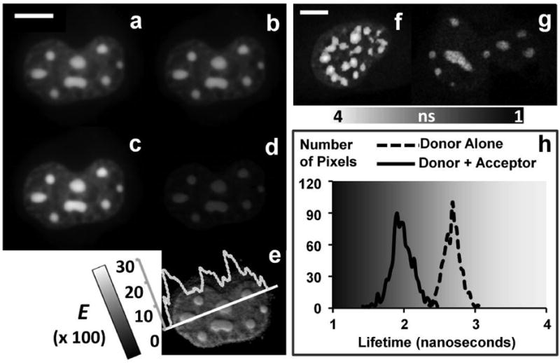
Fluorescent signals from the nucleus of a cell co-expressing CFP-C/EBPα (donor (D)) and YFP-C/EBPα (acceptor (A)) were measured in the D (a), A (b) and FRET (c) channels in wide-field microscopy. The processed FRET (PFRET, d) and apparent FRET efficiency (E%, e) images were obtained after processing the data with the PFRET algorithm in combination of the images acquired from the single-label expressing cells (see Section 4.1.2). The interaction between CFP- and YFP-tagged C/EBPα is demonstrated by the E% images and indicates the homo-dimerization of C/EBPα in regions of centromeric heterochromatin of cell nucleus. The same biological system was also studied using a time correlated single photon counting (TCSPC) FLIM-FRET method, where the unquenched (τ_D = 2.68 ns) and quenched (τ_DA = 1.98 ns) donor lifetimes were determined from cells only expressing CFP--C/EBPα (f and the dash line in h) and cells that co-express CFP-C/EBPα and YFP-C/EBPα (g and the solid line in h). The FRET efficiency (E = 26.12%), determined from “1 - τ_DA / τ_D”, confirms the results obtained in the intensity-based wide-field FRET measurements. (Wide-field images were acquired by an Olympus IX70 microscope equipped with a 60X/1.2NA water objective lens and a CCD camera (Hamamatsu Orca2). The donor and acceptor excitation wavelengths were selected from the X-Cite ^® 120 fluorescence illumination system (www.exfo-xcite.com) using 436/20 nm and 500/20 nm band-pass filters, respectively. The 470/30 nm and 535/30 nm band-pass filters were used to for the donor and acceptor emission channels, respectively. The TCSPC FLIM system and data analysis were described in detail earlier ^[65]. Data was acquired using the Becker & Hickl SPC-730 module on the Biorad Radiance 2100 confocal/multiphoton imaging system coupled to a Nikon TE 300 microscope equipped with a Nikon 60×/1.4NA water objective lens. Specimens were excited by a multi-photon laser tuned to 820 nm and the CFP signals were collected using a fast PMT (PMH-100, Becker & Hickl) with a 480/30 nm band-pass filter. Scale bar = 10 μm in both case.)

4.1.3 Spectral FRET Microscopy

Spectral imaging microscopy ^[66-69] produces λ-stacks consisting of x-, y- (spatial) and λ- (spectral) dimensions, measuring the emission signals in a series of spectral intervals equally sampled over a spectral range, at each pixel location. This is an ideal technique to implement FRET imaging in living cells and establishing the existence of a FRET signal ‘on-the-fly’. Linearly unmixing a D-A λ-stack based on the reference spectra obtained from D-alone and A-alone control specimens can separate the signals emitted from D and A. Therefore, after linear unmixing the FRET signals are only contaminated by the acceptor SBT signals since both are characterized by the spectrum of the acceptor fluorophore. Employing the same strategy of correcting the acceptor SBT used in the PFRET method, we developed the spectral FRET (sFRET) algorithm ^[50]. There are also other sFRET methods using confocal or two-photon spectral imaging microscopy in combination of linear unmixing ^[70-72]. Although sFRET imaging is usually more time consuming (in data acquisition for different λs) than filter-based FRET imaging, which is more suitable for 3-D or time-lapse FRET studies ^[73], the detailed spectral information generated by sFRET imaging provides a very accurate means of separating the donor SBT signals from the FRET signals ^[67]. Since both the D and the A reference spectra can be obtained beforehand for online unmixing of a D-A λ-stack, an online quantitative sFRET imaging and analysis routine can be easily implemented if the acceptor SBT can be ignored - this is possible by choosing a FRET pair where A is barely excited at the D excitation wavelength ^[72].

4.2 Donor Dequenching

Measuring the intensities of an identical donor fluorophore in the absence (I_D) and the presence (I_DA) of A can directly yield the energy transfer efficiency (E) based on Equation 4.

$$E=1-\frac{{\text{I}}_{\text{DA}}}{{\text{I}}_{\text{D}}}$$ (4)

Based on this principle, two microscopy imaging methods were used:

4.2.1 Acceptor Photobleaching (AP) FRET Microscopy

In AP-FRET microscopy, the D intensities are measured before (I_DA) and after (I_D) photobleaching A in a specimen containing both ^[74-76], the specimen serving as its own control. While widely used and serving as an excellent verification technique, this method is generally unsuitable for live-cell imaging and has also shown some photo conversion artifacts. ^[77].

4.2.2 Photoquenching (PQ) FRET Microscopy

PQ-FRET takes advantage of photo-activatable GFP (turned to a bright fluorescent state from an original dark fluorescent state upon a brief UV excitation) ^[78] acting as A and measures the D (CFP) signals before (I_D) and after (I_DA) activating the A ^[79]. Besides FRET, one can also monitor the diffusion of the activated acceptor fluorophores over time after one shot of activation in a small region. Thus, the PQ-FRET assay provides direct measurements of protein mobility, exchange and interactions in living cells ^[79].

4.3 Fluorescence Lifetime Imaging (FLIM)

Fluorescence lifetime refers to the average time a molecule stays in its excited state before emitting a photon and is an intrinsic property of a fluorophore. Fluorescence lifetime measurements started in early 1870 ^[80] in the context of phosphorescence (or delayed fluorescence). The first nanosecond lifetime imaging using optical microscopy was first implemented in 1959 using a frequency-domain method ^[81]. Since then, numerous methodologies both in frequency domain and time domain evolved for numerous biological and clinical applications ^{[6, 82]}. In the time domain, a fluorophore is usually excited with a pulsed-light source and its decay profile is directly measured at different time windows after each excitation pulse. The fluorescence lifetime of the fluorophore is estimated from analyzing the recorded decay profile. In the frequency domain, a modulated light source is used to excite a fluorophore, whose emission signals are measured by a detector modulated at the same frequency as the excitation light (Homodyne methods) or a frequency slightly (a few hundred to a few thousand hertz) different than the excitation light (Heterodyne methods) ^[83]. The fundamental frequency is chosen upon the lifetime scale of the fluorophore (megahertz for nanosecond decays). The phase shift(s) and amplitude attenuation(s) of the emission signal relative to the excitation source are analyzed to extract the fluorescence lifetime of the fluorophore.

One of the major FLIM applications is to measure FRET between fluorescent molecules ^{[7, 16, 65, 84-86]}, although the acceptor molecules need not be fluorescent. In FLIM-FRET microscopy, FRET events can be identified by measuring the reduction in the D lifetime that results from quenching in the presence of an acceptor. The energy transfer efficiency (E) can be estimated from the D lifetimes determined in the absence (τ_D – unquenched lifetime) and the presence (τ_DA – quenched lifetime) of the A (Equation 5) ^[6].

$$E=1-\frac{{\tau }_{\text{DA}}}{{\tau }_{\text{D}}}$$ (5)

An example of using a time correlated single photon counting (TCSPC) FLIM-FRET microscopy method to detect the dimerization of C/EBPα in the living pituitary cell nucleus ^[65] is shown in Figure 4f-h, which confirms the result obtained from the intensity-based FRET measurements (see Section 4.1.2). In FLIM-FRET microscopy, spectral bleedthrough is usually not an issue since only the donor signals are monitored, and fluorescence lifetime is not influenced by probe concentration, excitation light intensity, or light scattering; these facts make FLIM-FRET microscopy an accurate method for FRET measurements. The early FLIM systems were expensive and primarily custom-built in biophysics laboratories. In the past ten years, commercial FLIM systems have become available, from Becker & Hickl (www.becker-hickl.de), Picoquant (www.picoquant.com), ISS (www.iss.com), Lambert Instruments (www.lambert-instruments.com) and Intelligent Imaging Innovations (www.intelligent-imaging.com). These systems can be stand alone or integrated with existing multiphoton or confocal or wide-field microscopy systems for various applications. Acquiring enough photons is usually required for accurate estimation of the fluorescence lifetime. Thus, data acquisition in FLIM microscopy may take a few seconds to several minutes depending on the expression level of a fluorophore and the configuration of a FLIM system.

4.4 Fluorescence Polarization Anisotropy

For a randomly oriented population of fluorophores excited by linearly polarized light, the ones with its absorption dipole oriented parallel to the polarization axis are preferentially excited. In fluorescence polarization microscopy, the photons emitted from fluorophores excited by a linearly polarized light source are measured using two linear polarizer filters – one is parallel to the direction of the polarized excitation (I_‖) and the other is perpendicular to that direction (I_⊥). The anisotropy value (r) determined by Equation 6 measures the degree of the fluorophore orientation.

$$r=\frac{{\text{I}}_{\parallel }-{\text{I}}_{\perp }}{{\text{I}}_{\parallel }{+2\text{I}}_{\perp }}$$ (6)

The anisotropy value (r) will decrease (called depolarization) if the fluorophore changes its orientation which can be caused by FRET, providing the basic concept for using fluorescence anisotropy to measure FRET. Although the fluorophore rotation can also change its orientation, this effect can usually be ignored since energy transfer takes place more rapidly than the motion, especially for fluorescent proteins which are large and rotate slowly ^{[8, 35]}. Both, steady-state and time-revolved fluorescence anisotropy imaging methods have been developed for FRET studies ^[87-94]. It should be noted that energy transfer can occur between two identical fluorophores – called homo-FRET. Fluorescence anisotropy is the only method capable of measuring homo-FRET, which has been used to measure monomer-dimer transition of GFP-tagged proteins ^[87] and quantify protein cluster sizes with sub-cellular resolution ^[93]. Although fluorescence anisotropy imaging can be an excellent technique for distinguishing FRET and no FRET, quantitative discrimination of the FRET significance can be difficult with this approach, since the depolarization (used to indicate FRET) can also be induced by the instrumentation parameters, such as the objective lens – significant depolarization can be observed by using a higher numerical aperture lens ^{[8, 94]}.

4.5 Calibration of FRET techniques using FRET standards

As described above, numerous FRET microscopy methods have been developed and many of them have the capability to interpret the change in proximity between D and A through measuring the energy transfer efficiency (E). However, it has been difficult to compare the accuracies of the different methods. An elegant solution to this problem is the development of a set of genetic constructs encoding fusion proteins containing donor and acceptor FPs separated by protein linkers of defined length ^{[70, 95]}. For each genetic construct expressed in living cells, there was consensus in the E results obtained by different FRET microscopy methods ^[95], demonstrating that they could serve as FRET standards. We also compared various FRET microscopy techniques and assessed their utilities using four Cerulean (C)-Venus (V) based FRET standard constructs expressed in living cells ^[96] – C5V, C17V, C32V where C and V are tethered by either a 5, 7 or 32 amino acid linker ^[95], and CTV where C and V are separated by a 229 amino acid linker encoding a TRAF domain ^[70]. The photophysical properties of C and V, their Förster distance are given in Table 1.

Figure 5a shows the E comparison of the four FRET-standard constructs measured by spectral FRET (sFRET), time correlated single photon counting (TCSPC) FLIM-FRET and frequency-domain (FD) FLIM-FRET methods ^[96]. For sFRET, the raw spectral graphs are compared as well as the calculated E images (see Figure 5b). For TCSPC FLIM-FRET, the recorded decays are compared as well as the distributions of the estimated lifetimes (see Figure 5c). For FD FLIM-FRET, a phasor (or polar) plot approach ^{[97, 98]} is used to demonstrate the difference between the constructs (see Figure 5d). Each method is capable of characterizing the different distances in the linked Cerulean-Venus pairs based on E, the results are closely matched, confirming that these FRET-standard constructs expressed in live cells can serve as reference specimens to calibrate a particular FRET microscopy imaging technique.

Figure 5. Comparison of FRET measurements of Cerulean (C)-Venus (V) based FRET-standard constructs (CTV, C32V, C17V, C5V) expressed in living cells in spectral FRET (sFRET), time correlated single photon counting (TCSPC) and frequency-domain (FD) FLIM-FRET microscopy (see Section 4.5).

(a) The average FRET efficiencies (E%) of the four FRET-standard constructs measured in all three methods are compared as columns with error bars being standard deviations (n = 12 for each construct measured in each method). (b) In sFRET microscopy, it is clearly observed from the raw spectral graphs that the ratio of the V peak to the C peak increases from CTV to C5V, indicating an increase in E% in the same direction. The quantitative confirmation is shown by the representative E% images obtained after processing the data with the sFRET algorithm (see Section 4.1.3). (c) shows the representative C-alone and FRET-standard decay profiles (at one pixel of each cell) and lifetime distributions (in each cell) obtained in the TCSCP FLIM-FRET measurements, clearly demonstrating a faster decay (a shorter lifetime) from C to C5V. (d) displays the phasor plots ^{[97, 98]} of the representative cells expressing C only or the FRET-standard constructs (20MHz, Semicircle - Single Lifetime Curve; (1,0) - Zero Lifetime; (0,0) - Infinite Lifetime), which also clearly indicate a longer lifetime from C5V to C. (The details about these measurements were described earlier ^[96]. Briefly, sFRET imaging was carried out on a Zeiss 510 Meta imaging system coupled to a Zeiss Axiovert 200M microscope equipped with a Zeiss 63X/1.4NA oil objective lens. The Argon 458 nm and 514 nm laser lines were used as the donor and acceptor excitations, respectively. The emission signals were acquired in the spectrum of 458∼651 nm at 10.7 nm intervals. The TCSPC FLIM data was acquired using the Becker Hickl SPC-150 module on the Biorad Radiance 2100 confocal/multiphoton imaging system coupled to a Nikon TE 300 microscope equipped with a Nikon 60×/1.4NA water objective lens. Specimens were excited by a multi-photon laser tuned to 820 nm and the Cerulean signals were collected using a fast PMT (PMC-100-0, Becker & Hickl) with a 480/30 nm band-pass filter. The FD FLIM measurements were carried on the ISS ALBA system coupled to a Nikon TiU microscope equipped with a Nikon 60×/1.4NA water objective lens. Specimens were excited by a 440 nm pulsed diode laser and the Cerulean signals were collected using an avalanche photodiode (APD) with a 480/30 nm band-pass filter. The phase shifts and amplitude attenuations were measured at five frequencies - 20, 40, 60, 80, 100 MHz.)

5. Three-Color Fret Microscopy

Employing a traditional 2-color FRET method to determine the inter-relationships of three cellular components (A, B, C) would require the sequential imaging and analysis of the FRET-pair combinations of AB, BC and AC. A simplified 3-color FRET analysis system would be of great benefit to determine protein complex assemblies during signaling events, trafficking dynamics, or cytokinesis, particularly in the context of treatments, which may alter the relationship of the three components of interest. Most 3-color FRET publications have dealt with in-vitro studies in solutions using fluorometry or spectroscopy to detect components labeled by organic dyes for medical diagnostic ^{[26, 99-104]}. Besides ensemble-based assays, 3-color FRET has also been employed for single-molecule studies ^{[27, 105-107]}. To study processes in living cells, a 3-color FRET method (3-FRET) was developed using a combination of Cyan, Yellow and monomeric Red fluorescent proteins in wide-field microscopy ^[108]. However, this particular 3-FRET method is essentially an adaptation of 2-color FRET methodology to the three possible FRET pairings, since it used both double- and single-labeled control specimens, as well as acceptor photobleaching of the most red-shifted FP in the triple-labeled specimens, to determine individual FRET efficiencies ^[108]. This 3-FRET study lacked modeling to thoroughly describe the energy transfer events and efficiencies in the three-chromophore system based on the used microscopy imaging technique, which is essential to the development of a straightforward and robust 3-color FRET microscopy method.

Recently, we designed a 3-color FRET model based on the detection of the sensitized emissions from acceptors through steady-state imaging ^[109]. This model (described by Figure 6) has three symbolic fluorophores: F1 (donor), F2 (acceptor to F1 and donor to F3), and F3 (acceptor), assuming the spectral overlap (donor emission-acceptor excitation) of each pair (F1-F2, F1-F3, F2-F3) is sufficient for FRET to occur. Ex1, Ex2, and Ex3 are the one-photon peak excitation wavelengths for F1, F2, and F3, respectively. At Ex1, the following energy transfer events are possible: F1 (donor) is excited and transfers energy directly to F2 (acceptor) at E₁₂ (the energy transfer efficiency characterizing the spatial relationship between F1 and F2) and also to F3 (acceptor) at E₁₃ (the energy transfer efficiency characterizing the spatial relationship between F1 and F3); F2 (acceptor to F1 and donor to F3) can directly absorb Ex1 and be sensitized due to the energy transfer from F1 (donor), and then transfers energy to F3 (acceptor) at E₂₃ (the energy transfer efficiency characterizing the spatial relationship between F2 and F3). At Ex2, the three-fluorophore system excited by Ex2 becomes a 2-color FRET system, where F2 transfers energy to F3 at the same E₂₃, assuming that under experimental conditions Ex2 does not excite F1 to any noticeable degree. At Ex3, there is no FRET event, assuming that under experimental conditions Ex3 does not excite F1 and F2 to produce a noticeable signal.

Figure 6. Three-color FRET model.

(a) F1, F2, and F3 represent the excitation (dashed line) and emission (solid line) for the three fluorophores; the spectral overlap (donor emission and acceptor excitation) of each pair (F1-F2, F1-F3, F2-F3) is sufficient for FRET to occur. (b) Exciting the three-fluorophore system with Ex1 (solid lines), direct absorption and energy transfer occurs in parallel: F1→F2 at an energy transfer efficiency E₁₂ and F1→F3 at an energy transfer efficiency E₁₃; In addition, F2 (excited by Ex1 and sensitized due to the energy transfer F1→F2) also transfers energy to F3 at an energy transfer efficiency E₂₃. At Ex2, the three-fluorophore system (dashed lines) becomes a 2-color (F2-F3) FRET system with F2 transferring energy to F3 at the same energy transfer efficiency E₂₃. There is no energy transfer in the three-fluorophore system at Ex3 excitation. All of the above is based on the validated assumptions that the absorption rates of F1 at Ex2 or Ex3 and of F2 at Ex3 are trivial or not apparent.

In our 3-color spectral FRET (3sFRET) approach we used confocal spectral imaging microscopy to acquire λ-stacks from the triple-labeled (F1-F2-F3) and the single-labeled (F1, F2, F3) specimens, applied linear unmixing to separate the emitted signals of the three fluorophores, and finally employed an algorithm-based software to process the unmixed images to determine the corrected FRET signals and apparent E₁₂, E₁₃ and E₂₃ ^[109]. The FRET-standard approach was used to validate the 3sFRET microscopy method. Three different fluorescent proteins (FP) - mTFP, Venus and tdTomato (see Table 1) - were linked to each other to generate a 3-color FRET-standard construct. In addition, three different 2-FP combinations, each tethered in the same way as the 3-FP construct, were generated. The 2-FP reference constructs were analyzed using our established 2-color spectral FRET microscopy method (see Section 4.1.3) to compare with the apparent Es of the 3-FP construct processed in 3sFRET microscopy (see Figure 7), assuming the spatial relationships between FPs in the 2-FP reference constructs were the same as those in the 3-FP construct, verified by fluorescence lifetime measurements ^[109]. Once validated, the 3sFRET microscopy method was applied to characterize the interactions between the dimerized transcription factor CCAAT/enhancer binding protein alpha (C/EBPα) and the heterochromatin protein-1 alpha (HP1α) in live mouse pituitary cells ^[109]. An additional algorithm, applied to 3-color FRET in wide-field or conventional confocal microscopy was also developed and incorporated into a software package (see Supporting Material in Ref. [109]). Figure 8 shows an example of employing the 3-color FRET approach in conventional confocal microscopy to simultaneously detect the homo-dimerization of C/EBPα and its interaction with H1Pα in a single living mouse pituitary GHFT1 cell.

Figure 7. Validation of the 3-color spectral FRET (3sFRET) microscopy method using FRET-standard constructs.

To validate the 3sFRET method, three fluorescent proteins (FP) – mTFP, Venus and tdTomato (see Table 1) were used to build a 3-FP FRET-standard construct, where mTFP was coupled to Venus by a 5 amino acid (aa) linker and Venus was further tethered with tdTomato by a 10 aa linker, resulting in an mTFP-5aa-Venus-10aa-tdTomato complex. In addition, three 2-FP FRET-standard constructs were also generated: mTFP-5aa-Venus, Venus-10aa-tdTomato and mTFP-5aa-Amber-10aa-tdTomato, where Amber is a non-fluorescent mutant form of Venus (Y66C) ^[95], used in the 2-FP construct to maintain the same spatial relationship between mTFP and tdTomato as in the 3-FP construct. (a) is the overlay of the spectral images obtained from a cell expressing the 3-FP construct excited at the 458 nm wavelength and (b) shows the representative spectra of the cell sequentially excited at three different wavelengths, which were chosen around the peak excitation wavelengths of mTFP (458 nm), Venus (514 nm) and tdTomato (561 nm). The apparent FRET efficiencies (E%) between FPs in the 3-FP construct measured in 3sFRET microscopy - E₁₂% (E% between mTFP and Venus, c), E13% (E% between mTFP and tdTomato, d) and E23% (E% between Venus and tdTomato, e), were validated by the E%s of the 2-FP constructs measured using an established 2-color spectral FRET microscopy method ^[50]: (f) mTFP-5aa-Venus, (g) mTFP-5aa-Venus-10aa- tdTomato and (h) Venus-5aa-tdTomato. (The details about the validation are described in Ref. [109]. Briefly, 3sFRET and two-color sFRET imaging was carried out on a Zeiss 510 Meta imaging system coupled to a Zeiss Axiovert 200M microscope equipped with a Zeiss 63X/1.4NA oil objective lens. The Argon 458 nm, 514 nm laser lines and diode-pumped solid-state 561 nm laser were used as the mTFP, Venus and tdTomato excitations, respectively. The emission signals were acquired in the spectrum of 469∼651 nm at 10.7 nm intervals. Scale bar = 10 μm.)

Figure 8. Demonstration of the homo-dimerization of CCAAT/enhancer-binding protein alpha (C/EBPα) and its interaction with heterochromatin protein 1 α (HP1α) in live mouse pituitary cell nucleus by 3-color confocal FRET Microscopy.

Cells expressing mTFP- C/EBPα, Venus-C/EBPα and tdTomato-HP1α (see Table 1) were sequentially excited by three different wavelengths, which were chosen around the peak excitation (Ex) wavelengths of mTFP (Ex1), Venus (Ex2) and tdTomato (Ex3); the emitted signals were measured in three separate emission (Em) channels (mTFP: Em1, Venus: Em2, tdTomato: Em3), resulting the 6-channel images (a: Ex1-Em1, b: Ex1-Em2, c: Ex1-Em3, d: Ex2-Em2, e: Ex2-Em3 and f: Ex3-Em3). The images were then processed by the 3-color FRET algorithm, together with the images acquired from the single-label (mTFP-C/EBPα, Venus-C/EBPα and tdTomato-HP1α) control specimens in those 6 channels, to obtain the apparent FRET efficiency (E%) images (g: E% between mTFP and Venus, h: E% between mTFP and tdTomato, i: E% between Venus and tdTomato). The interactions between mTFP-C/EBPα, Venus-C/EBPα and tdTomato-HP1α are demonstrated by the 3-color E% images and indicate homo-dimerization of C/EBPα and the association between the C/EBPα dimer and HP1α in regions of heterochromatin of the cell nucleus. See Ref. [109] for more data analysis of this biological model in 3-color spectral FRET microscopy. (Confocal imaging was carried out on a Leica SP5 × white light laser (WLL) system ^[32] coupled to a Leica DMI6000 microscope equipped with a Leica 63×/1.4NA oil objective lens. The Argon 458 nm (Ex1), 514 nm (Ex2) and WLL 550 nm (Ex3) laser lines were used as the mTFP, Venus and tdTomato excitations, respectively. The mTFP (Em1 = 470∼500 nm), Venus (Em2 = 525∼550 nm) and tdTomato (Em3 = 560∼650 nm) emission channels were configured using the Leica acousto-optical beam splitter (AOBS). Scale bar = 10 μm.)

Our studies have demonstrated the utility of the 3-color FRET microscopy method for characterizing the interactions between the three fluorescent proteins in living cells ^[109], making it a promising live cell imaging technique for broad applications in cell biology and other life-science applications. However, it should also be recognized that the optimization of the biological system to allow efficient and balanced expression of the three different labeled proteins might be a significant limitation to the 3-color FRET approach, although this is a general problem for FRET-based studies and varies depending on the biological system. In the 3-color FRET model, we only considered the F1-F2, F1-F3 and F2-F3 energy transfer pathways in a three-fluorophore (F1-F2-F3) system. There might be some other energy pathways existing in such a complicated system composed of multiple donors and acceptors ^[110]. While the 3-color FRET algorithm does not require double-labeled (F1-F2, F1-F3, F2-F3) specimens, it is sensible to initially prepare those double-labeled FRET pairs, check their spectral properties and verify that F1 interacts with F2 and/or F3, and that F2 interacts with F3, and to finally evaluate these results with those obtained in 3-color FRET microscopy.

Currently, we are using 3-color confocal FRET microscopy and the combination of mTFP, Venus and monomeric Red or Cherry FP to investigate the dynamic interactions of IQGAP1, Rac1, CDC42 and actin during polymerization of actin. We believe that 3-color FRET microscopy can be extended to other suitable fluorescent proteins, fluorescent organic dyes as conjugates, or antibody staining and quantum dots. The method can be tailored to handle a particularly designed three-fluorophore (F1-F2-F3) system - e.g. a system composed of two parallel energy transfer pathways where F1 interacts simultaneously with two independent acceptors (F2 and F3), meaning that there is no interaction between F2 and F3; or a system only composed of a sequential energy transfer pathway: F1 to F2 then to F3, where the intermediate fluorophore (F2) acts as an acceptor for F1 and upon sensitization becomes the donor for F3. Either situation would be suitable for example for signaling complexes, where multiple proteins assemble upon stimulation, which could be tracked in four dimensions (x, y, z, t). Furthermore, the relative distances established by 3-color FRET between three labeled components, and their changes over time, could provide valuable insights into the dynamics of the interaction.

6. Summary and Outlook

FRET has had a major impact already in the life sciences, drug development and medicine. We imaging has clearly moved mainstream, it is not a trivial methodology and still presents many obstacles to a successful outcome, which however can be mastered. Optimizing all the variables is a considerable challenge: the suitability of imaging targets (cells, tissue, proteins, lipids, nano structures etc), choice of fluorophores, instruments and different techniques, plus the extremely valuable extension of FRET imaging to include quantitative analysis rather than just qualitative parameters. Based on the history of the past two decades, we can predict that there will be dramatic new developments in the next two decades taking Theodor Förster's theory to new heights. These developments will happen on all fronts: new fluorophores with improved characteristics, expanding the choice of suitable FRET partners; more sophisticated instruments with faster acquisition time to capture rapid dynamic cellular processes, routine SBT-corrected data generation on-the-fly, easy single-molecule tracking, quantitative high-content FRET screening arrays; improved algorithms to manage the many variables in FRET microscopy to achieve even higher levels of accuracy. For sure, Theodor Förster's legacy will be apparent for many decades to come.

References

- 1.Förster T. Naturwissenschafien. 1946;6:166–175. [Google Scholar]
- 2.Clegg RM. In: Reviews in fluorescence. Geddes CD, Lakowicz JR, editors. Springer; New York: 2006. pp. 1–45. [Google Scholar]
- 3.Gilmore AM, Larkum AW, Salih A, Itoh S, Shibata Y, Bena C, Yamasaki H, Papina M, Van Woesik R. Photochem Photobiol. 2003;77:515–523. doi: 10.1562/0031-8655(2003)077<0515:strote>2.0.co;2. [DOI] [PubMed] [Google Scholar]
- 4.Förster T. In: modern quantum chemistry. Sinanoglu O, editor. Academic Press Inc.; 1965. pp. 93–137. [Google Scholar]
- 5.Clegg RM. In: Fluorescence imaging spectroscopy and microscopy. Wang XF, Herman B, editors. John Wiley & Sons Inc.; New York: 1996. pp. 179–251. [Google Scholar]
- 6.Lakowicz JR. Principles of fluorescence spectroscopy. Springer; New York: 2006. [Google Scholar]
- 7.Wallrabe H, Periasamy A. Curr Opin Biotechnol. 2005;16:19–27. doi: 10.1016/j.copbio.2004.12.002. [DOI] [PubMed] [Google Scholar]
- 8.Piston DW, Kremers GJ. Trends Biochem Sci. 2007;32:407–414. doi: 10.1016/j.tibs.2007.08.003. [DOI] [PubMed] [Google Scholar]
- 9.Shaner NC, Lin MZ, McKeown MR, Steinbach PA, Hazelwood KL, Davidson MW, Tsien RY. Nat Methods. 2008;5:545–551. doi: 10.1038/nmeth.1209. [DOI] [PMC free article] [PubMed] [Google Scholar]
- 10.Day RN, Schaufele F. J Biomed Opt. 2008;13:031202. doi: 10.1117/1.2939093. [DOI] [PubMed] [Google Scholar]
- 11.Day RN, Davidson MW. Chem Soc Rev. 2009;38:2887–2921. doi: 10.1039/b901966a. [DOI] [PMC free article] [PubMed] [Google Scholar]
- 12.Wallrabe H, Elangovan M, Burchard A, Periasamy A, Barroso M. Biophys J. 2003;85:559–571. doi: 10.1016/S0006-3495(03)74500-7. [DOI] [PMC free article] [PubMed] [Google Scholar]
- 13.Wallrabe H, Bonamy G, Periasamy A, Barroso M. Mol Biol Cell. 2007;18:2226–2243. doi: 10.1091/mbc.E06-08-0700. [DOI] [PMC free article] [PubMed] [Google Scholar]
- 14.Mills JD, Stone JR, Rubin DG, Melon DE, Okonkwo DO, Periasamy A, Helm GA. J Biomed Opt. 2003;8:347–356. doi: 10.1117/1.1584443. [DOI] [PubMed] [Google Scholar]
- 15.Li H, Li HF, Felder RA, Periasamy A, Jose PA. J Biomed Opt. 2008;13:031206. doi: 10.1117/1.2943286. [DOI] [PMC free article] [PubMed] [Google Scholar]
- 16.Li H, Yu P, Sun Y, Felder R, Periasamy A, Jose P. J Biomed Opt. 2010;15:056003. doi: 10.1117/1.3484751. [DOI] [PMC free article] [PubMed] [Google Scholar]
- 17.Algar WR, Krull UJ. Anal Bioanal Chem. 2008;391:1609–1618. doi: 10.1007/s00216-007-1703-3. [DOI] [PubMed] [Google Scholar]
- 18.Resch-Genger U, Grabolle M, Cavaliere-Jaricot S, Nitschke R, Nann T. Nat Methods. 2008;5:763–775. doi: 10.1038/nmeth.1248. [DOI] [PubMed] [Google Scholar]
- 19.Zhong W. Anal Bioanal Chem. 2009;394:47–59. doi: 10.1007/s00216-009-2643-x. [DOI] [PubMed] [Google Scholar]
- 20.Medintz IL, Mattoussi H. Phys Chem Chem Phys. 2009;11:17–45. doi: 10.1039/b813919a. [DOI] [PubMed] [Google Scholar]
- 21.Moshinsky DJ, Ruslim L, Blake RA, Tang F. J Biomol Screen. 2003;8:447–452. doi: 10.1177/1087057103255282. [DOI] [PubMed] [Google Scholar]
- 22.Zhou V, Han S, Brinker A, Klock H, Caldwell J, Gu XJ. Anal Biochem. 2004;331:349–357. doi: 10.1016/j.ab.2004.04.011. [DOI] [PubMed] [Google Scholar]
- 23.Xu Z, Nagashima K, Sun D, Rush T, Northrup A, Andersen JN, Kariv I, Bobkova EV. J Biomol Screen. 2009;14:1257–1262. doi: 10.1177/1087057109349356. [DOI] [PubMed] [Google Scholar]
- 24.Periasamy A, Siadat-Pajouh M, Wodnicki P, Wang XF, Herman B. Microscopy and Analysis. 1995:19–21. [Google Scholar]
- 25.Lundin K, Blomberg K, Nordstrom T, Lindqvist C. Anal Biochem. 2001;299:92–97. doi: 10.1006/abio.2001.5370. [DOI] [PubMed] [Google Scholar]
- 26.Watrob HM, Pan CP, Barkley MD. J Am Chem Soc. 2003;125:7336–7343. doi: 10.1021/ja034564p. [DOI] [PubMed] [Google Scholar]
- 27.Hohng S, Joo C, Ha T. Biophys J. 2004;87:1328–1337. doi: 10.1529/biophysj.104.043935. [DOI] [PMC free article] [PubMed] [Google Scholar]
- 28.Nagai T, Ibata K, Park ES, Kubota M, Mikoshiba K, Miyawaki A. Nat Biotechnol. 2002;20:87–90. doi: 10.1038/nbt0102-87. [DOI] [PubMed] [Google Scholar]
- 29.Rizzo MA, Springer GH, Granada B, Piston DW. Nat Biotechnol. 2004;22:445–449. doi: 10.1038/nbt945. [DOI] [PubMed] [Google Scholar]
- 30.Ai HW, Henderson JN, Remington SJ, Campbell RE. Biochem J. 2006;400:531–540. doi: 10.1042/BJ20060874. [DOI] [PMC free article] [PubMed] [Google Scholar]
- 31.Day RN, Booker CF, Periasamy A. J Biomed Opt. 2008;13:031203. doi: 10.1117/1.2939094. [DOI] [PMC free article] [PubMed] [Google Scholar]
- 32.Sun Y, Booker CF, Kumari S, Day RN, Davidson M, Periasamy A. J Biomed Opt. 2009;14:054009. doi: 10.1117/1.3227036. [DOI] [PMC free article] [PubMed] [Google Scholar]
- 33.Jares-Erijman EA, Jovin TM. Nat Biotechnol. 2003;21:1387–1395. doi: 10.1038/nbt896. [DOI] [PubMed] [Google Scholar]
- 34.Sekar RB, Periasamy A. J Cell Biol. 2003;160:629–633. [Google Scholar]
- 35.Vogel SS, Thaler C, Koushik SV. Sci STKE. 2006;2006:re2. doi: 10.1126/stke.3312006re2. [DOI] [PubMed] [Google Scholar]
- 36.Ponsioen B, Zhao J, Riedl J, Zwartkruis F, van der Krogt G, Zaccolo M, Moolenaar WH, Bos JL, Jalink K. EMBO Rep. 2004;5:1176–1180. doi: 10.1038/sj.embor.7400290. [DOI] [PMC free article] [PubMed] [Google Scholar]
- 37.Allen MD, DiPilato LM, Rahdar M, Ren YR, Chong C, Liu JO, Zhang J. ACS Chemical Biology. 2006;1:371–376. doi: 10.1021/cb600202f. [DOI] [PubMed] [Google Scholar]
- 38.Gao X, Zhang J. Mol Biol Cell. 2008;19:4366–4373. doi: 10.1091/mbc.E08-05-0449. [DOI] [PMC free article] [PubMed] [Google Scholar]
- 39.Tomida T, Takekawa M, O'Grady P, Saito H. Mol Cell Biol. 2009;29:6117–6127. doi: 10.1128/MCB.00571-09. [DOI] [PMC free article] [PubMed] [Google Scholar]
- 40.Vinkenborg JL, Nicolson TJ, Bellomo EA, Koay MS, Rutter GA, Merkx M. Nat Methods. 2009;6:737–740. doi: 10.1038/nmeth.1368. [DOI] [PMC free article] [PubMed] [Google Scholar]
- 41.Tron L, Szollosi J, Damjanovich S, Helliwell SH, Arndt-Jovin DJ, Jovin TM. Biophys J. 1984;45:939–946. doi: 10.1016/S0006-3495(84)84240-X. [DOI] [PMC free article] [PubMed] [Google Scholar]
- 42.Matyus L. J Photochem Photobiol B. 1992;12:323–337. doi: 10.1016/1011-1344(92)85039-w. [DOI] [PubMed] [Google Scholar]
- 43.Kam Z, Volberg T, Geiger B. J Cell Sci. 1995;108(Pt 3):1051–1062. doi: 10.1242/jcs.108.3.1051. [DOI] [PubMed] [Google Scholar]
- 44.Gordon GW, Berry G, Liang XH, Levine B, Herman B. Biophys J. 1998;74:2702–2713. doi: 10.1016/S0006-3495(98)77976-7. [DOI] [PMC free article] [PubMed] [Google Scholar]
- 45.Hoppe A, Christensen K, Swanson JA. Biophys J. 2002;83:3652–3664. doi: 10.1016/S0006-3495(02)75365-4. [DOI] [PMC free article] [PubMed] [Google Scholar]
- 46.Elangovan M, Wallrabe H, Chen Y, Day RN, Barroso M, Periasamy A. Methods. 2003;29:58–73. doi: 10.1016/s1046-2023(02)00283-9. [DOI] [PubMed] [Google Scholar]
- 47.van Rheenen J, Langeslag M, Jalink K. Biophys J. 2004;86:2517–2529. doi: 10.1016/S0006-3495(04)74307-6. [DOI] [PMC free article] [PubMed] [Google Scholar]
- 48.Zal T, Gascoigne NR. Biophys J. 2004;86:3923–3939. doi: 10.1529/biophysj.103.022087. [DOI] [PMC free article] [PubMed] [Google Scholar]
- 49.Periasamy A, Chen Y, Elangovan M. In: Molecular imaging: FRET microscopy and spectroscopy. Periasamy A, Day RN, editors. Oxford University Press; New York: 2005. pp. 126–145. [Google Scholar]
- 50.Chen Y, Mauldin JP, Day RN, Periasamy A. J Microsc. 2007;228:139–152. doi: 10.1111/j.1365-2818.2007.01838.x. [DOI] [PMC free article] [PubMed] [Google Scholar]
- 51.Youvan DC, Silva CM, Bylina EJ, Coleman WJ, Dilworth MR, Yang MM. Biotechnology Et Alia. 1997:1–18. [Google Scholar]
- 52.Mahajan NP, Linder K, Berry G, Gordon GW, Heim R, Herman B. Nat Biotechnol. 1998;16:547–552. doi: 10.1038/nbt0698-547. [DOI] [PubMed] [Google Scholar]
- 53.Kraynov VS, Chamberlain C, Bokoch GM, Schwartz MA, Slabaugh S, Hahn KM. Science. 2000;290:333–337. doi: 10.1126/science.290.5490.333. [DOI] [PubMed] [Google Scholar]
- 54.Sorkin A, McClure M, Huang F, Carter R. Curr Biol. 2000;10:1395–1398. doi: 10.1016/s0960-9822(00)00785-5. [DOI] [PubMed] [Google Scholar]
- 55.Xia Z, Liu Y. Biophys J. 2001;81:2395–2402. doi: 10.1016/S0006-3495(01)75886-9. [DOI] [PMC free article] [PubMed] [Google Scholar]
- 56.Jin T, Yue L, Li J. J Biol Chem. 2001;276:12879–12884. doi: 10.1074/jbc.M010513200. [DOI] [PubMed] [Google Scholar]
- 57.Zal T, Zal MA, Gascoigne NR. Immunity. 2002;16:521–534. doi: 10.1016/s1074-7613(02)00301-1. [DOI] [PubMed] [Google Scholar]
- 58.Hailey DW, Davis TN, Muller EG. Methods Enzymol. 2002;351:34–49. doi: 10.1016/s0076-6879(02)51840-1. [DOI] [PubMed] [Google Scholar]
- 59.Berney C, Danuser G. Biophys J. 2003;84:3992–4010. doi: 10.1016/S0006-3495(03)75126-1. [DOI] [PMC free article] [PubMed] [Google Scholar]
- 60.Chen Y, Periasamy A. J Fluoresc. 2006;16:95–104. doi: 10.1007/s10895-005-0024-1. [DOI] [PubMed] [Google Scholar]
- 61.Chen H, Puhl HL, 3rd, Koushik SV, Vogel SS, Ikeda SR. Biophys J. 2006;91:L39–41. doi: 10.1529/biophysj.106.088773. [DOI] [PMC free article] [PubMed] [Google Scholar]
- 62.Wallrabe H, Chen Y, Periasamy A, Barroso M. Microsc Res Tech. 2006;69:196–206. doi: 10.1002/jemt.20281. [DOI] [PubMed] [Google Scholar]
- 63.Schaufele F, Demarco IA, Day RN. In: Molecular imaging: FRET microscopy and spectroscopy. Periasamy A, Day RN, editors. Oxford University Press; New York: 2005. pp. 72–94. [Google Scholar]
- 64.Sun Y, Periasamy A. J Biomed Opt. 2010;15:020513. doi: 10.1117/1.3407655. [DOI] [PMC free article] [PubMed] [Google Scholar]
- 65.Chen Y, Periasamy A. Microsc Res Tech. 2004;63:72–80. doi: 10.1002/jemt.10430. [DOI] [PubMed] [Google Scholar]
- 66.Dickinson ME, Bearman G, Tille S, Lansford R, Fraser SE. BioTechniques. 2001;31:1272, 1274–6, 1278. doi: 10.2144/01316bt01. [DOI] [PubMed] [Google Scholar]
- 67.Zimmermann T, Rietdorf J, Girod A, Georget V, Pepperkok R. FEBS Lett. 2002;531:245–249. doi: 10.1016/s0014-5793(02)03508-1. [DOI] [PubMed] [Google Scholar]
- 68.Zimmermann T, Rietdorf J, Pepperkok R. FEBS Lett. 2003;546:87–92. doi: 10.1016/s0014-5793(03)00521-0. [DOI] [PubMed] [Google Scholar]
- 69.Zimmermann T. Adv Biochem Eng Biotechnol. 2005;95:245–265. doi: 10.1007/b102216. [DOI] [PubMed] [Google Scholar]
- 70.Thaler C, Koushik SV, Blank PS, Vogel SS. Biophys J. 2005;89:2736–2749. doi: 10.1529/biophysj.105.061853. [DOI] [PMC free article] [PubMed] [Google Scholar]
- 71.Megias D, Marrero R, Martinez Del Peso B, Garcia MA, Bravo-Cordero JJ, Garcia-Grande A, Santos A, Montoya MC. Microsc Res Tech. 2009;72:1–11. doi: 10.1002/jemt.20633. [DOI] [PubMed] [Google Scholar]
- 72.Raicu V, Stoneman MR, Fung R, Melnichuk M, Jansma DB, Pisterzi LF, Rath S, Fox M, Wells JW, Saldin DK. Nat Photon. 2009;3:107–113. [Google Scholar]
- 73.Hoppe AD, Shorte SL, Swanson JA, Heintzmann R. Biophys J. 2008;95:400–418. doi: 10.1529/biophysj.107.125385. [DOI] [PMC free article] [PubMed] [Google Scholar]
- 74.Kenworthy AK. Methods. 2001;24:289–296. doi: 10.1006/meth.2001.1189. [DOI] [PubMed] [Google Scholar]
- 75.Day RN, Voss TC, Enwright JF, 3rd, Booker CF, Periasamy A, Schaufele F. Mol Endocrinol. 2003;17:333–345. doi: 10.1210/me.2002-0136. [DOI] [PMC free article] [PubMed] [Google Scholar]
- 76.Kenworthy AK. In: Molecular imaging: FRET microscopy and spectroscopy. Periasamy A, Day RN, editors. Oxford University Press; New York: 2005. pp. 146–164. [Google Scholar]
- 77.Kremers GJ, Hazelwood KL, Murphy CS, Davidson MW, Piston DW. Nat Methods. 2009;6:355–358. doi: 10.1038/nmeth.1319. [DOI] [PMC free article] [PubMed] [Google Scholar]
- 78.Patterson GH, Lippincott-Schwartz J. Science. 2002;297:1873–1877. doi: 10.1126/science.1074952. [DOI] [PubMed] [Google Scholar]
- 79.Demarco IA, Periasamy A, Booker CF, Day RN. Nat Methods. 2006;3:519–524. doi: 10.1038/nmeth889. [DOI] [PMC free article] [PubMed] [Google Scholar]
- 80.Phipson TL. Phosphorescence or the emission of light by minerals, plants and animals. L Reeve & Co; London: 1870. [Google Scholar]
- 81.Venetta BD. Review of Scientific Instruments. 1959;30:450–457. [Google Scholar]
- 82.Periasamy A, Clegg RM, editors. FLIM microscopy in biology and medicine. CRC Press; London: 2009. [Google Scholar]
- 83.Spring BQ, Clegg RM. In: FLIM microscopy in biology and medicine. Periasamy A, Clegg RM, editors. CRC Press; London: 2009. pp. 117–144. [Google Scholar]
- 84.Wouters FS, Bastiaens PI. Curr Biol. 1999;9:1127–1130. doi: 10.1016/s0960-9822(99)80484-9. [DOI] [PubMed] [Google Scholar]
- 85.Chen Y, Mills JD, Periasamy A. Differentiation. 2003;71:528–541. doi: 10.1111/j.1432-0436.2003.07109007.x. [DOI] [PubMed] [Google Scholar]
- 86.Biener E, Charlier M, Ramanujan VK, Daniel N, Eisenberg A, Bjorbaek C, Herman B, Gertler A, Djiane J. Biol Cell. 2005;97:905–919. doi: 10.1042/BC20040511. [DOI] [PubMed] [Google Scholar]
- 87.Gautier I, Tramier M, Durieux C, Coppey J, Pansu RB, Nicolas JC, Kemnitz K, Coppey-Moisan M. Biophys J. 2001;80:3000–3008. doi: 10.1016/S0006-3495(01)76265-0. [DOI] [PMC free article] [PubMed] [Google Scholar]
- 88.Clayton AH, Hanley QS, Arndt-Jovin DJ, Subramaniam V, Jovin TM. Biophys J. 2002;83:1631–1649. doi: 10.1016/S0006-3495(02)73932-5. [DOI] [PMC free article] [PubMed] [Google Scholar]
- 89.Lidke DS, Nagy P, Barisas BG, Heintzmann R, Post JN, Lidke KA, Clayton AH, Arndt-Jovin DJ, Jovin TM. Biochem Soc Trans. 2003;31:1020–1027. doi: 10.1042/bst0311020. [DOI] [PubMed] [Google Scholar]
- 90.Mattheyses AL, Hoppe AD, Axelrod D. Biophys J. 2004;87:2787–2797. doi: 10.1529/biophysj.103.036194. [DOI] [PMC free article] [PubMed] [Google Scholar]
- 91.Rizzo MA, Piston DW. Biophys J. 2005;88:L14–6. doi: 10.1529/biophysj.104.055442. [DOI] [PMC free article] [PubMed] [Google Scholar]
- 92.Piston DW, Rizzo MA. Methods Cell Biol. 2008;85:415–430. doi: 10.1016/S0091-679X(08)85018-2. [DOI] [PubMed] [Google Scholar]
- 93.Bader AN, Hofman EG, Voortman J, en Henegouwen PM, Gerritsen HC. Biophys J. 2009;97:2613–2622. doi: 10.1016/j.bpj.2009.07.059. [DOI] [PMC free article] [PubMed] [Google Scholar]
- 94.Vogel SS, Thaler C, Blank PS, Koushik SV. In: FLIM microscopy in biology and medicine. Periasamy A, Clegg RM, editors. CRC Press; London: 2009. pp. 245–288. [Google Scholar]
- 95.Koushik SV, Chen H, Thaler C, Puhl HL, 3rd, Vogel SS. Biophys J. 2006;91:L99–L101. doi: 10.1529/biophysj.106.096206. [DOI] [PMC free article] [PubMed] [Google Scholar]
- 96.Sun Y, Seo SA, Provence S, Periasamy A. In: Proc SPIE. Periasamy A, So PTC, Konig K, editors. Vol. 7569. SPIE; San Francisco: 2010. p. 75690Z. [Google Scholar]
- 97.Redford GI, Clegg RM. J Fluoresc. 2005;15:805–815. doi: 10.1007/s10895-005-2990-8. [DOI] [PubMed] [Google Scholar]
- 98.Digman MA, Caiolfa VR, Zamai M, Gratton E. Biophys J. 2008;94:L14–6. doi: 10.1529/biophysj.107.120154. [DOI] [PMC free article] [PubMed] [Google Scholar]
- 99.Ramirez-Carrozzi VR, Kerppola TK. Proc Natl Acad Sci U S A. 2001;98:4893–4898. doi: 10.1073/pnas.091095998. [DOI] [PMC free article] [PubMed] [Google Scholar]
- 100.Liu J, Lu Y. J Am Chem Soc. 2002;124:15208–15216. doi: 10.1021/ja027647z. [DOI] [PubMed] [Google Scholar]
- 101.Haustein E, Jahnz M, Schwille P. Chemphyschem. 2003;4:745–748. doi: 10.1002/cphc.200200634. [DOI] [PubMed] [Google Scholar]
- 102.Heinze KG, Jahnz M, Schwille P. Biophys J. 2004;86:506–516. doi: 10.1016/S0006-3495(04)74129-6. [DOI] [PMC free article] [PubMed] [Google Scholar]
- 103.Klostermeier D, Sears P, Wong CH, Millar DP, Williamson JR. Nucleic Acids Res. 2004;32:2707–2715. doi: 10.1093/nar/gkh588. [DOI] [PMC free article] [PubMed] [Google Scholar]
- 104.Aneja A, Mathur N, Bhatnagar PK, Mathur PC. J Biol Phys. 2008;34:487–493. doi: 10.1007/s10867-008-9107-y. [DOI] [PMC free article] [PubMed] [Google Scholar]
- 105.Heilemann M, Tinnefeld P, Sanchez Mosteiro G, Garcia Parajo M, Van Hulst NF, Sauer M. J Am Chem Soc. 2004;126:6514–6515. doi: 10.1021/ja049351u. [DOI] [PubMed] [Google Scholar]
- 106.Clamme JP, Deniz AA. Chemphyschem. 2005;6:74–77. doi: 10.1002/cphc.200400261. [DOI] [PubMed] [Google Scholar]
- 107.Lee NK, Kapanidis AN, Koh HR, Korlann Y, Ho SO, Kim Y, Gassman N, Kim SK, Weiss S. Biophys J. 2007;92:303–312. doi: 10.1529/biophysj.106.093211. [DOI] [PMC free article] [PubMed] [Google Scholar]
- 108.Galperin E, Verkhusha VV, Sorkin A. Nat Methods. 2004;1:209–217. doi: 10.1038/nmeth720. [DOI] [PubMed] [Google Scholar]
- 109.Sun Y, Wallrabe H, Booker CF, Day RN, Periasamy A. Biophys J. 2010;99:1274–1283. doi: 10.1016/j.bpj.2010.06.004. [DOI] [PMC free article] [PubMed] [Google Scholar]
- 110.Koushik SV, Blank PS, Vogel SS. PLoS One. 2009;4:e8031. doi: 10.1371/journal.pone.0008031. [DOI] [PMC free article] [PubMed] [Google Scholar]
Associated Data
This section collects any data citations, data availability statements, or supplementary materials included in this article.