Adjusting confounders in ranking biomarkers: a model-based ROC approach

Abstract

High-throughput studies have been extensively conducted in the research of complex human diseases. As a representative example, consider gene-expression studies where thousands of genes are profiled at the same time. An important objective of such studies is to rank the diagnostic accuracy of biomarkers (e.g. gene expressions) for predicting outcome variables while properly adjusting for confounding effects from low-dimensional clinical risk factors and environmental exposures. Existing approaches are often fully based on parametric or semi-parametric models and target evaluating estimation significance as opposed to diagnostic accuracy. Receiver operating characteristic (ROC) approaches can be employed to tackle this problem. However, existing ROC ranking methods focus on biomarkers only and ignore effects of confounders. In this article, we propose a model-based approach which ranks the diagnostic accuracy of biomarkers using ROC measures with a proper adjustment of confounding effects. To this end, three different methods for constructing the underlying regression models are investigated. Simulation study shows that the proposed methods can accurately identify biomarkers with additional diagnostic power beyond confounders. Analysis of two cancer gene-expression studies demonstrates that adjusting for confounders can lead to substantially different rankings of genes.

INTRODUCTION

In the study of complex human diseases, such as cancer, diabetes and cardiovascular diseases, clinical risk factors and environmental exposures have been shown to have insufficient predictive power for diagnosis and prognosis prediction [1]. High-throughput studies have been conducted, aiming to profile human genome and search for biomarkers with additional diagnostic power. To avoid confusion of terminology, in this article, we use microarray gene-expression profiling study as a representative example, though the proposed approach has many applications beyond gene-expression study. In gene-expression studies, an important goal is to identify and rank gene expressions with additional diagnostic power beyond clinical risk factors and environmental exposures [2].

Denote Y as the response variable and as the q gene expressions to be ranked, with . For each subject, a set of p confounders U (clinical risk factors and environmental exposures) are measured, with . For example in cancer studies, U may include variables such as age, gender, race, medication history, exposure to radiation and others. Compared with gene expressions, clinical and environmental risk factors have a lower dimensionality, can be more easily and accurately measured, and have more important implications for public health. In addition, some of such risk factors are modifiable, making them more relevant to clinical practice.

Many published studies adopt a model-based ranking approach and proceed as follows: (i) for gene k( = 1 , … , q), fit a statistical model , where ϕ is a pre-specified parametric or semi-parametric model; (ii) based on the fitted model, compute a ranking statistic r_k for gene k( = 1 , … , q); (iii) rank biomarkers based on the magnitudes of r_ks. Consider, for example, a diagnosis study with binary response. A commonly adopted model ϕ is the logistic regression model, and the ranking statistic can be taken as the absolute value of regression coefficient estimate, its significance level or value of the maximized likelihood function. When standard regression models (e.g. logistic model for binary response, Cox model for survival response) are adopted, such an approach can be easily extended to accommodate effects of confounders. The most impressive feature of this approach is its computational simplicity. However, the aforementioned ranking statistics all measure estimation significance, which is not a direct measure of diagnostic accuracy. Recent studies, such as [3] and references therein, have shown that with high-throughput data, there is no one-to-one correspondence between estimation significance and diagnostic accuracy. The difference can be significant when the sample size is not large and there are many biomarkers.

As an alternative to the aforementioned approach, ROC approaches directly evaluate the differential ability of biomarkers [4]. In addition, they are able to focus on the whole spectrum of specificity and sensitivity and provide lucid interpretations. Pepe et al. [5] and Ma and Song [6] use ROC approaches to rank diagnostic performance of biomarkers with binary and survival response variables, respectively. However, those studies focus on biomarkers only and ignore the effects of confounders. Intuitively, it is possible to follow a strategy similar to the model-based approach described above and extend [5, 6] to accommodate confounders in biomarker ranking. However, such an extension encounters computational difficulties. Without making any normality assumption on the biomarkers (which usually does not hold with practical data), the empirical ROC objective function is not continuous. Maximizing such an objective function demands either computationally extensive searching or functional approximation [7]. To the best of our knowledge, there is still a lack of numerical method that is computationally affordable and generically applicable.

Our goal is to develop a ROC-based ranking approach, which can identify and rank the diagnostic accuracy of biomarkers while properly adjusting for confounders. The proposed approach advances from the existing model-based ranking approach by directly evaluating diagnostic accuracy and from the existing ROC approach by accommodating confounders. It, hence, can be more informative than existing approaches. Furthermore, the proposed approach is readily implemented in existing software packages and computationally affordable, since its computational complexity is linear in terms of the number of biomarkers in data.

METHODS

When confounders U are present, ranking the q biomarkers X₁ , … , X_q follows a strategy similar to that with model-based ranking described in the above section. However, there are two key differences. The first is that for gene k, the statistical model is . Challenge arises as the effect of U needs to be modeled and estimated q times, each time with a different X_k. The second difference is that the ranking statistic is now taken as a ROC-based measure, which is more informative than estimation significance. In the following subsections, we investigate gene-expression data with binary and censored survival responses separately.

Adjustment with binary response variable

Consider a diagnosis study, where Y = 0/1 denotes the presence/absence of a certain disease or two different stages of the same disease. The proposed approach can be easily extended to accommodate categorical responses with multiple levels following [8] by replacing area under the ROC curve (AUC) with volume under the multi-dimensional ROC surface.

We first ignore confounders and consider gene expressions only. For gene k( = 1 , … , q), consider the logistic regression model

(1)

where π = P(Y = 1|X_k), β₀ and β_k denote the unknown intercept and regression coefficient, respectively. Denote as the maximum likelihood estimate (MLE) of (β₀,β_k) based on n independent and identically distributed (iid) subjects. For subject i, in the sample, we can make a model-based diagnostic decision by calculating the predicted probability of a positive outcome as

and declaring that the predicted outcome to be one or zero according to whether the value of is greater or less than a threshold t∈(0,1). The set can now be viewed as a sample for a ‘diagnostic marker’ . For a fixed threshold t, the sensitivity and specificity of π^k are

respectively. The curve of se_k versus 1 − across all t values is called the ROC curve [4]. An overall summary measure is the area under the ROC curve (AUC) which is defined as . AUC has the probability interpretation of , which facilitates a relatively simpler way to estimate AUC by

(2)

When the effects of confounders are ignored, {AUC^k:k=1 , … , q} can be used to rank biomarkers, with larger AUC values indicating higher diagnostic accuracy. We refer to this method as M₀ (method of no-adjustment) hereafter. This method has been adopted in [5] for binary response and [6] for survival response. With M₀, rankings using π^k and X_k as diagnostic markers are identical because of the invariance of AUC under monotone increasing transformations. Therefore, there is actually no need to fit regression models to obtain this type of ranking. Moreover, even with no adjustment for confounders, there are multiple possible ways of ranking biomarkers. One instant example is to simply rank, the P-values of estimated β_ks from (1). However, we have observed from numerical studies that this method performs quite similar to M₀ (details omitted). Intuitively, we expect that there exists very limited room to find more effective methods for ranking biomarkers without properly accounting for the effects of confounders.

Method M₁: individual adjustment

We now consider a more realistic model, where π depends on not only X but also U. In particular, for gene k, we extend model (1) as

(3)

where β₁ is the length-p vector of unknown regression coefficients. For subject i, we can obtain its individual covariate-adjusted risk represented by

where are the MLEs of the regression coefficients in (3). We then calculate the AUC value for gene k by regarding as the diagnostic marker values and applying a similar formula as (2).

With this adjustment method, the effect of confounders is estimated q times, each time with a different gene. This strategy has been commonly adopted with simple model-based approaches. The q estimates of confounder coefficients are usually different. This may cause difficulty in interpreting the effects of confounders (e.g. when the signs of a confounder are different in different models) and in making a fair comparison across the q genes. Such a concern motivates the development of the following two adjustment methods, which have the same confounding effect estimate in all of the q regression models.

Method M₂: marginal adjustment

We propose first fitting the logistic model

(4)

which involves the confounders only. Denote the MLE of as (). For gene k, we then consider the logistic regression model

where β_2k is the only unknown parameter and is considered as the known offset value in the model. Denote the MLE of β_2k as . For subject i, the marginal covariate-adjusted risk is then given by

The rest of the ranking procedure is the same as described above.

With method M₂, the confounding effect is estimated in the absence of genes and then kept constant in downstream analysis. It measures the ‘net’ effect of confounders, which is the main quantity of interest in classic epidemiologic studies. Compared with M₁, different genes are now compared on a more common ground. The computational complexity of this method is similar to that of M₀.

The development of complex human diseases is associated with the combined effects of confounders and multiple genes. Thus, a more sensible data generating model assumes that

(5)

where is the whole set of biomarkers. Marginal ranking of biomarkers amounts to marginalization of the above joint model by focusing on one gene at a time. From the joint-modeling perspective, the estimate of β₁ and hence effect of confounders should be generated in the presence of X. Motivated by such a consideration, we propose the following method.

Method M₃: joint adjustment

We first fit regression model (5). Denote ) as a proper estimate of . With this estimate, the rest of the ranking procedure is the same as that with method M₂.

When n ≫ q + p, can be obtained from simple likelihood approaches. However, with gene-expression data, usually n≪q. Thus a straightforward MLE is not attainable. To facilitate practical implementation, we propose a screening-based penalization approach, which proceeds as follows.

1. Apply method M₀. That is, for gene k( = 1 , … , q), calculate its AUC value without adjusting for confounders. Rank the q genes using their unadjusted AUC values;

2. Select the top κ genes from the sorted list of genes to be X in model (5);

3. Fit model (5) with a penalized logistic regression approach and obtain .

With recent development in regularized estimation (e.g. penalization) methods, it is possible to fit a joint-regression model with confounders and all genes. Among the thousands of profiled genes, only few are expected to have diagnostic power for the response. Recent studies, such as [9], suggest that marginal screening in Step (1) may not only reduce computational cost for penalized estimation but also more importantly lead to more accurate estimates. Theoretically speaking, a partial orthogonality condition can guarantee the consistency of screening. The goal of the screening is to conduct a rough selection. Thus, κ should not be too small. In our numerical study, we set κ ∼ n, as it is expected that the number of genes with diagnostic power to be much smaller. Data-driven methods such as cross-validation can be used to determine κ, however, may lead to higher computational cost. Compared with sample size, the number of confounders and genes passed screening may be comparable or larger. Thus, penalized estimation, which can effectively stabilize the estimation, is needed in Step (3). With generalized linear models, several penalization approaches can be adopted. Comprehensive overviews of the development of these approaches and their properties can be found in [10–14] and many others. In our numerical study, penalized Bregman divergence with deviance loss in [13] and the adaptive Lasso approach in [14] are adopted for gene-expression data with binary and censored survival responses respectively.

Remarks

An important characteristic of ROC approaches is that they are ‘model-free’. The proposed approach needs to fit logistic regression models and thus may suffer from model mis-specification. There are studies, such as [7, 15], advocating using AUC as the objective function for building composite diagnostic markers. The binormal AUC function relies on the normality assumption, which usually does not hold with gene-expression data. The empirical AUC objective function is a sum of indicator functions. In practice, computationally expensive searching or approximation is needed for optimization. We have experienced with some of the available computational approaches and found that they either have prohibitively high-computational cost or tend to perform poorly when there are a few covariates (e.g. more than five). Because of the computational concerns, we turn to the proposed model-based approach. The logistic regression model is the most widely adopted model for binary data. If there is evidence in favor of other models (e.g. probit model), the proposed approach can be easily extended.

Adjustment with survival response variable

For survival response variable, the status of a subject at each time point is binary (death or alive). The ROC curve and the corresponding AUC can be constructed at each time point. A single measure of diagnostic accuracy can then be obtained by integrating AUC over the time. We refer to [16] and others for the development of time-dependent ROC techniques.

With survival response variable, the most commonly adopted model is the Cox proportional hazards model. With slight abuse of notation, we continue to denote by Y the survival outcome in this section. The Cox model assumes that , where and denote the hazard function and the baseline hazard function at time y, respectively; β is the regression coefficient for a generic covariate X (which can be a confounder or a gene). The partial likelihood estimation of β can be obtained by existing software packages, such as coxph in R, stcox in STATA or PROC PHREG in SAS. After fitting the model, let be the hazard score for subject i. A larger value of corresponds to a higher level of hazard and shorter survival time predicted based on X_i. Thus, we can treat as if they were a set of diagnostic markers.

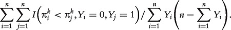
With survival response variable Y and a generic diagnostic marker η, a commonly implemented diagnostic accuracy summary measure is the time-integrated AUC [17] defined as

where η_j is the diagnostic test statistic and Y_j is the corresponding survival time for the jth subject (j = 1, 2) randomly sampled from the population. A larger value of C indicates that a greater value of η is associated with a shorter survival Y more often than not. This time-integrated AUC measures the concordance between η and Y and can be used to rank markers. This definition also facilitates a simple formula to estimate the time-integrated AUC as

(6)

In survival analysis, observations are often subject to censoring. Some data sets even have a mixture of different types of censoring. Thus, not all pairs of (Y_i,Y_j) have a definitive order. Some pairs of observations are less informative than others. We refer to a recent study [18] for detailed algorithms for computing, the time-integrated AUC under various censoring scenarios (omitted here for brevity). With the Cox model and above definition of time-integrated AUC, adjusting for confounders can follow the same strategy as with binary data. All the three proposed adjustments, individual adjustment, marginal adjustment and joint adjustment, can be conducted.

AUC by refitted cross-validation

In the approach described above, the model fitting and AUC calculation are carried out using the same data. When the sample size is not very large, and there are a number of covariates, there is a concern of over-fitting and hence overly optimistic diagnostic measure. We propose a refitted cross-validation procedure in AUC evaluation, following the strategy in [19]. The procedure proceeds as follows:

1. For a data set with n subjects, randomly split into two sets with equal sizes referred to as set I and set II;

2. With binary (survival) data, construct the logistic (Cox) model using set I. Apply the fitted model from set I, make a prediction for subjects in set II, and compute AUC_I, the ranking AUCs for set II;

3. Repeat Step 2 by exchanging the roles of set I and set II, and construct the ranking AUCs referred to as AUC_II;

4. Use (AUC_I + AUC_II)/2 as the ranking statistics.

To avoid bias caused by an extreme partition, repeat the above process multiple times and take the average AUCs as the ranking statistics.

SIMULATION

Binary response variable

We simulate 100 sets of gene-expression data. In each set, there are n = 100 iid subjects. Subject i has a binary outcome Y_i, q = 19 995 gene expressions X_i = (X_1,i , … , X_q,i)^T and P = 5 confounding covariates U_i = (U_1,i , … , U_p,i)^T. , i = 1, … , n are simulated as iid random vectors, where 0_q+p denotes the (q + p) × 1 zero vector, Σ=diag(Σ₁,Σ₂,Σ₃), where Σ₁, i = 1, 2, 3, are symmetric matrices with diagonal elements set equal to 1 and off-diagonal elements equal to 0.4; Σ₁, and respectively have dimensions , 5 × 5 and . We generate the binary response via

(7)

(8)

where β₀ = 1, β₁ = (2, 2, 1, 1, 1)^T, β₂ = (, 0.5, 0.5, 0.5, 0.5, 1.5, 1.5, 1.5, )^T.

That is, for each subject, we simulate five confounding covariates U₁ , … , U₅ and 19 995 gene expressions X₁ , … , X₁₉₉₉₅. The regression coefficients of U₁,U₂ are set as 2, whereas those of as 1. Gene expressions are simulated as having a three-group structure. Genes within the same groups have a compound-symmetry correlation structure with correlation coefficient 0.4, and genes within different groups are independent. In group one, X₁ , … , X₅₀ are simulated as not associated with response, i.e. β_2,k = 0, for k = 1 , … , 50. These genes are correlated with the confounding covariates. In group two, X₅₁ , … , X₅₇ are simulated as associated with response, with regression coefficients in (7) set as 0.5, 0.5, 0.5, 0.5, 1.5, 1.5, 1.5. In group three, X₅₈ , … , X₁₉₉₉₅ are not associated with response. In addition, genes in groups two and three are not correlated with confounding covariates.

We apply the four methods to simulated data. With 100 replicates, we compute the frequencies that genes are ranked in top 20 by different methods. In Table 1, we show the frequencies for seven important genes as well as those for seven randomly selected unimportant genes that are correlated with confounders. As can be seen from Table 1, for important genes, the three proposed adjustment methods significantly outperform the commonly adopted M₀ by ranking them much more frequently in top 20. The performances of the three proposed methods are ordered as M₁ < M₂ < M₃ as expected, though the difference is not dramatic. From the second part of Table 1, we can see that the no-adjustment method, which is still commonly adopted, may rank unimportant genes that happen to be correlated with confounders in the top. Such genes represent ‘redundant’ information given confounders, are of significantly less interest, and should be ranked low. The three proposed methods can effectively solve this problem. For unimportant genes not correlated with confounders, all four methods have almost zero frequencies ranking them in top 20 (detailed results omitted).

Table 1:

Simulation study with binary response: frequencies of genes ranked in the top 20 out of 100 datasets

	X51	X52	X53	X54	X55	X56	X57
M0	40	32	32	39	64	75	67
M1	68	69	66	64	93	85	88
M2	68	71	74	76	93	90	92
M3	66	73	79	83	95	95	93
	X16	X19	X22	X27	X28	X32	X34
M0	24	29	35	33	28	27	33
M1	0	0	1	0	0	0	1
M2	0	0	1	1	0	0	0
M3	0	0	1	1	0	1	0

Genes X₅₁… X₅₇ are associated with response; Genes X₁₆, X₁₉, X₂₂, X₂₇, X₂₈, X₃₂ and X₃₄ are not associated with response but correlated with confounders.

Scatter plots of AUCs are constructed to further illustrate efficacy of the proposed methods in gene ranking. The upper four panels of Figure 1 display the scatter plots of the AUCs of X₄₁ (which does not have diagnostic power but is correlated with confounders) versus those of X₅₄ (which has diagnostic power but is not correlated with confounders) for the 100 simulated data sets. Since X₄₁ is simulated as unimportant whereas X₅₄ as important, an effective method is expected to result in larger AUC values for X₅₄ than those for X₄₁. Consequently, the majority of the points in Figure 1 should be below the 45° reference line; and the more the points deviate from this line, the better the method. The upper four panels of Figure 1 show that with M₀, the points are ‘randomly’ scattered around the reference line, suggesting that the AUCs of and X₅₄ are similar and this method cannot effectively distinguish between the relative importance of these two genes. The proposed three methods, on the other hand, can effectively solve this problem. In particular, almost all points are located below the reference lines, suggesting that with the proposed methods, gene X₅₄ can be ranked as having more diagnostic power than gene X₄₁. Similar phenomena are observed with other pairs of genes (details omitted). The lower four panels of Figure 1 present the scatter plots of the AUCs of versus those of X₅₉₈ (a randomly selected unimportant gene not correlated with confounders). Now that as both genes are unimportant, an effective method should yield points centered on the 45° reference line. The lower four panels of Figure 1 show that the three proposed adjustment methods are able to achieve such a property, while the no-adjustment method tends to have larger AUC values for gene X₄₁.

Figure 1:

Simulation study with binary response. Upper four panels: AUC of X₄₁ vs. X₅₄. Lower four panels: AUC of X₄₁ vs. X₅₉₈. Solid green line: 45° reference line.

Survival response variable

We simulate 100 sets of gene-expression data. In each set, there are n = 150 iid subjects. Each subject has 5995 gene expressions and five confounding covariates. The regression coefficients of confounders are set as (1, 1, 1, 1, 1)^T, and the regression coefficients of important genes are set as (0.5, 0.5, 0.5, 0.5, 1, 1, 1)^T. The values of other parameters as well as the procedures of generating U₁ , … , U_p, X₁ , … , X_q are the same as those for binary response data. Following [20], we generate the survival outcomes (Y_i,C_i) of subject i as

where ; is the inverse cumulative hazard function of the Weibull distribution, λ = 1,ν = 2; serves as the time of censoring for subject i. The censoring rate is about 39%.

Gene ranking results of different methods are presented in Table 2. The observations are similar to those made in Table 1, with the proposed adjustment methods significantly outperforming the no-adjustment method. A difference from Table 1 is that here with the seven important genes, we observe no difference among the three proposed methods. Scatter plots similar to those in Figure 1 are obtained. We omit the figure for presentational brevity.

Table 2:

Simulation study with survival response: frequencies of genes ranked in the top 20 out of 100 datasets

	X51	X52	X53	X54	X55	X56	X57
M0	63	62	60	63	88	82	84
M1	100	100	99	100	100	100	100
M2	100	100	99	100	100	100	100
M3	100	100	99	100	100	100	100
	X16	X19	X22	X27	X28	X32	X34
M0	24	29	31	35	28	30	27
M1	0	2	1	3	0	0	1
M2	0	0	2	1	1	0	0
M3	2	2	0	1	1	0	1

Genes X₅₁… X₅₇ are associated with response; Genes X₁₆, X₁₉, X₂₂, X₂₇, X₂₈, X₃₂ and X₃₄ are not associated with response but correlated with confounders.

Remark

More simulations are presented in Supplementary Data (available online at http://bib.oxfordjournals.org/). Conclusions similar to those above are drawn. In our simulation studies, methods and M₃ lead to similar results. Both methods account for confounders with fixed offsets across all markers. In addition, as the ‘overall correlation’ between gene expressions and confounders is not dramatically strong, the fixed offset estimates under the two methods can be reasonably close. Performance of accuracy measures is expected to be stable under a uniform adjustment with accurately estimated offset. Method M₃ tends to perform the best since it incorporates more information from markers. In this method, the regression coefficients of confounders are estimated by a Lasso penalization method, which usually has sound asymptotic properties (see [10–14] and many others for references).

DATA ANALYSIS

Breast cancer study

Breast cancer is the second leading cause of deaths from cancer among women in the United States. Despite major progresses in breast cancer treatment, the ability to predict the metastatic behavior of tumor remains limited. The breast cancer study was first reported in [21]. Ninety-seven lymph node-negative breast cancer patients 55 years old or younger participated in this study. Among them, 46 developed distant metastases within 5 years (metastatic outcome coded as 1) and 51 remained metastases free for at least 5 years (metastatic outcome coded as 0). Clinical risk factors (confounders) collected include age, tumor size, histological grade, angioinvasion, lymphocytic infiltration, estrogen receptor (ER) and progesterone receptor (PR) status. Expression levels for 24 481 gene probes were collected. We remove genes with severe missingness, leading to an effective number of 24 188 genes.

We apply the four ranking methods. In Table 3, we provide the genes ranked in top 10 by methods M₀ and M₃ as well as corresponding rankings by other methods. We observe that the ranking by M₀ is significantly different from those by the three proposed methods, suggesting that adjusting for confounders can make a difference in practical gene ranking. The top ranked genes by methods M₁, M₂ and M₃ are more similar. However, we still observe a certain degree of difference. Such a difference is not surprising considering what is observed in simulation (Table 1). Considering the formulation of these methods and our simulation results, we recommend ranking by M₃ as the final ranking.

Table 3:

Analysis of breast cancer data: genes ranked in top 10 by methods M₀ (left) and M₃ (right) and corresponding rankings by other methods

Genes	Rankings by method				Genes	Rankings by method
	M0	M1	M2	M3		M0	M1	M2	M3
10 755	1	120	58	31	271	944	8	1	1
16 274	2	436	239	160	403	92	1	2	2
13 143	3	3399	1562	303	8	4938	36	10	3
10 513	4	1701	9488	304	272	286	4	3	4
19 642	5	3450	5728	1991	1439	85	3	4	5
7374	6	1385	345	249	24 023	589	69	39	6
22 328	7	251	995	76	921	31	9	9	7
296	8	403	311	141	194	2897	24	12	8
11 285	9	319	5215	209	23 488	1697	13	7	9
4682	10	542	580	411	593	5941	7	8	10

Follicular lymphoma study

Follicular lymphoma is the second most common form of non-Hodgkin’s lymphoma, accounting for about 22% of all cases. A study was conducted to determine whether the survival risks of patients with follicular lymphoma can be predicted by the gene-expression profiles of tumors and standard clinical risk factors at diagnosis [22]. Fresh-frozen tumor-biopsy specimens and clinical data from 191 untreated patients who had received a diagnosis of follicular lymphoma between 1974 and 2001 were obtained. The median age at diagnosis was 51 years (range 23–81), and the median follow-up time was 6.6 years (range: less than 1.0–28.2). The median follow-up time among patients alive at last follow-up was 8.1 years. Eight records with missing survival information are excluded from the analysis. Clinical covariates measured include extra nodal site, age, normalized LDH, performance status, stage and IPI.1 (IPI = 2 or 3) and IPI.2 (IPI = 4 or 5). We remove subjects with missing clinical covariate measurements. A total of 156 subjects are included in analysis. Affymetrix U133A and U133B microarray gene-chips were used to measure gene-expression levels. A log2 transformation was first applied to the Affymetrix measurements. As genes with higher variations are of more interest, we filter the 44 928 gene-expression measurements with the following criteria: (1) the max expression value of each gene across 156 samples must be greater than the median max expressions; and (2) the max–min expressions should be greater than their median. 6506 out of 44 928 genes pass the above unsupervised screening.

Analysis results using the four different ranking methods are shown in Table 4. The overall pattern is similar to that in Table 3. We again observe that different rankings are obtained by adjusting for confounders. Unlike with the breast cancer data, the ranking by M₀ is more similar to those by adjustment methods. The rankings by M₂ and M₃ are closer to each other.

Table 4:

Analysis of follicular lymphoma data: genes ranked in top 10 by methods M₀ (left) and M₃ (right) and corresponding rankings by other methods

Genes	Rankings by method				Genes	Rankings by method
	M0	M1	M2	M3		M0	M1	M2	M3
357	1	3	1	1	357	1	3	1	1
5417	2	167	36	23	2345	180	15	3	2
5095	3	12	12	10	6267	11	57	18	3
4445	4	482	74	242	6271	102	2785	19	4
2391	5	136	140	115	3653	74	16	4	5
1232	6	231	197	55	5711	7	6	11	6
5711	7	6	11	6	5946	137	5	5	7
3625	8	70	47	11	6296	122	1	2	8
4769	9	652	180	386	1070	242	91	25	9
6060	10	317	725	186	5095	3	12	12	10

DISCUSSION

In high-throughput biomedical studies, there are two general strategies investigating high-dimensional biomarkers. The first is to study their joint effects in a single statistical model. In recent literature, a large amount of regularization studies have been conducted along this direction. The second is to study their marginal effects possibly in the presence of confounders but not other biomarkers. Most biological and clinical studies take this strategy. From a biological point of view, the development and progression of diseases are associated with the combined effects of confounders and multiple genes. Thus, the joint-effect strategy may seem more sensible. However, marginal analysis and ranking may provide insights not available in joint-effect analysis (e.g. streamlining genes for further investigation, or answering questions like ‘what is the optimal model if only one or a small number of genes are allowed in the model’), and thus can be of considerable importance.

In marginal ranking, while focusing only on biomarkers may be of some interest, more sensible ranking analysis should properly account for the effects of low-dimensional confounders, which may include clinical risk factors and environmental exposures in human disease research. In this article, we focus on ranking resulted from using AUC. It is noted that the proposed methods can be straightforwardly extended to using partial AUC [5] or weighted AUC [23] to accommodate scenarios where a subinterval of ROC curve should be taken into account or the area under the ROC curve should be considered under a weighted scheme. Because of the computational difficulty encountered by ROC approaches, we build composite diagnostic models/markers using a single gene and confounders based on parametric or semi-parametric regression models. Three different methods for adjusting confounders are developed. Our numerical studies suggest that (i) adjusting for confounders may lead to rankings significantly different from no-adjustment analysis; (ii) the proposed methods can better identify genes with additional diagnostic power beyond confounders; and (iii) out of the three proposed methods, M₃ is intuitively most reasonable and has the best performance. The proposed methods are computationally feasible and convenient to implement using existing software packages. For example, in R, the glm function in the base package and the coxph function in package survival can be used to fit, respectively, the logistic regression model and Cox model. The penalized estimation with method M₃ can be achieved with the function glmnet and others. The calculation of AUC can be achieved with functions auc (library pROC) for binary data and survivalROC (library survivalROC) for survival data. Computing code for this paper will be available from the authors upon request.

Ranking investigated in this article amounts to marginalize a certain joint data generating model. When there is no confounder, the marginalization is simple and uniquely defined. However, with the presence of confounders, there is not a clear way of marginalization. The three proposed methods are all intuitively reasonable and reflect different ways of marginalization. As discussed in previous sections, a limitation of the proposed analysis is that it builds diagnostic models via fitting certain parametric or semi-parametric regression models. Although, in theory, it is possible to build diagnostic models using a model-free ROC approach, in practice, we may encounter significant computational difficulties. The logistic and Cox models are adopted as they have been the default in the analysis of binary and survival data. To the best of our knowledge, there is a lack of rigorous model determination approach with high-dimensional data. In this study, we have focused on methodological development and investigated performance of the proposed methods via numerical study. For each gene, the validity of estimation and (time-integrated) AUC calculation is almost trivial. With a large number of genes, the uniform consistency of these estimates can be partly deduced from recent studies [24]. As the problem investigated is mostly of practical interest, we defer theoretical investigation to future study. The relative importance of genes is inferred from the AUC values. As a secondary analysis, it is possible to deduce the P-values of the AUCs and use them to assist ranking and selecting genes. The calculation of significance level may follow [18] or use bootstrap approaches. The scenarios presented in simulation are simpler than what is encountered in practice. We intentionally choose those settings to demonstrate that the proposed methods may lead to a big difference even under simple settings. In the real data analysis, we are able to show that the proposed methods lead to different rankings in practice. However, unlike with simulation data, we are unable to show whether the genes ranked in top by the proposed methods are ‘more meaningful’. In high-throughput studies, gene ranking is usually step one of the full analysis. Downstream analysis, e.g. functional analysis, is needed to fully quantify the association between genes and response.

In this article, we have focused on continuous biomarkers and two types of response variables—binary and censored survival. Some of the state-of-art data such as single nucleotide polymorphism (SNP) data may have discrete biomarkers. ROC based approaches are no longer directly applicable with such data. We leave out the research of adjusting confounders for such data for future study. Another type of common response variable is continuous. With continuous response, ROC-based approaches simplify to the well-known maximum rank correlation approaches [25]. With the link to rank estimation approaches, the proposed methods can be extended to continuous and other types of response variables.

SUPPLEMENTARY DATA

Supplementary data are available online at http://bib.oxfordjournals.org/.

Key Points.

• When ranking biomarkers, ROC approaches directly target diagnostic accuracy and can be more informative than fully model-based approaches.

• Because of computational difficulties, existing ROC approaches often ignore confounders in ranking high-throughput biomarkers.

• The proposed model-based ROC approach is intuitively reasonable and computationally affordable. It can better identify biomarkers with diagnostic power beyond confounders.

• Application of the proposed approach may lead to significantly different rankings with cancer genomic data.

FUNDING

This study has been supported in part by awards R-155-000-100-133 from National University of Singapore (T.Y.), ARF R-155-000-109-112 from the Academic Research Funding in Singapore (J.L.) and CA142774 from National Institute of Health, DMS0904181 from National Science Foundation, USA (S.M.).

Biographies

Tao Yu obtained his Ph.D. in Statistics from University of Wisconsin, Madison. He is an Assistant Professor in Department of Statistics and Applied Probability, National University of Singapore.

Jialiang Li obtained his Ph.D. in Statistics from University of Wisconsin, Madison. He is an Assistant Professor in Department of Statistics and Applied Probability and Duke-NUS Graduate Medical School, National University of Singapore, as well as a Scientist in Singapore Eye Research Institute.

Shuangge Ma obtained his Ph.D. in Statistics from University of Wisconsin, Madison. He is an Associate Professor in School of Public Health, Yale University.

References

- 1.Wald NJ, Morris JK. Assessing risk factors as potential screening tests: a simple assessment tool. Arch Intern Med. 2011;171:286–91. doi: 10.1001/archinternmed.2010.378. [DOI] [PubMed] [Google Scholar]
- 2.Knudsen S. Cancer Diagnostics with DNA Microarrays. Hoboken, NJ: Wiley; 2006. [Google Scholar]
- 3.Han X, Li Y, Huang J, et al. Identification of predictive pathways for non-Hodgkin lymphoma prognosis. Cancer Inform. 2010;9:281–92. doi: 10.4137/CIN.S6315. [DOI] [PMC free article] [PubMed] [Google Scholar]
- 4.Pepe MS. The Statistical Evaluation of Medical Tests for Classification and Prediction. Oxford: Oxford University Press; 2003. [Google Scholar]
- 5.Pepe MS, Longton G, Anderson GL, et al. Selecting differentially expressed genes from microarray experiments. Biometrics. 2003;59:133–42. doi: 10.1111/1541-0420.00016. [DOI] [PubMed] [Google Scholar]
- 6.Ma S, Song X. Ranking prognosis markers in cancer genomic studies. Brief Bioinform. 2011;12:33–40. doi: 10.1093/bib/bbq069. [DOI] [PMC free article] [PubMed] [Google Scholar]
- 7.Ma S, Huang J. Combining multiple markers for classification using ROC. Biometrics. 2007;63:751–7. doi: 10.1111/j.1541-0420.2006.00731.x. [DOI] [PubMed] [Google Scholar]
- 8.Ferri C, Hernandez-Orallo J, Salido MA. In Proceedings of 14th European Conference on Machine Learning. Croatia: Cavtat-Dubrovnik; 2003. Volume under the ROC surface for multi-class problems; pp. 108–20. [Google Scholar]
- 9.Fan J, Song R. Sure independence screening in generalized linear models with NP-dimensionality. Ann Stat. 2010;38:3567–604. [Google Scholar]
- 10.Tibshirani R. Regression shrinkage and selection via the Lasso. J Roy Stat SocSer B. 1996;58:267–88. [Google Scholar]
- 11.Zou H. The adaptive Lasso and its oracle properties. J Am Stat Assoc. 2006;101:1418–29. [Google Scholar]
- 12.Huang J, Ma S, Zhang CH. Technical Report 392. Department of Statistics and Actuarial Science, University of Iowa; 2008. The iterated Lasso for high-dimensional logistic regression. [Google Scholar]
- 13.Zhang CM, Yuan J, Chai Y. Penalized Bregman divergence for large-dimensional regression and classification. Biometrika. 2010;97(3):551–66. doi: 10.1093/biomet/asq033. [DOI] [PMC free article] [PubMed] [Google Scholar]
- 14.Zhang HH, Lu W. Adaptive lasso for Cox’s proportional hazards model. Biometrika. 2007;94:691–703. [Google Scholar]
- 15.Song X, Ma S. Penalized variable selection with U-estimates. J Nonparam Stat. 2010;22(4):499–515. doi: 10.1080/10485250903348781. [DOI] [PMC free article] [PubMed] [Google Scholar]
- 16.Heagerty P, Lumley T, Pepe M. Time-dependent ROC curves for censored survival data and a diagnostic marker. Biometrics. 2000;56:337–44. doi: 10.1111/j.0006-341x.2000.00337.x. [DOI] [PubMed] [Google Scholar]
- 17.Heagerty PJ, Zheng Y. Survival model predictive accuracy and ROC curves. Biometrics. 2005;61:92–105. doi: 10.1111/j.0006-341X.2005.030814.x. [DOI] [PubMed] [Google Scholar]
- 18.Li J, Ma S. Time-dependent ROC analysis under diverse censoring patterns. Stat Med. 2011;30:1266–77. doi: 10.1002/sim.4178. [DOI] [PubMed] [Google Scholar]
- 19.Fan J, Guo S, Hao N. Variance estimation using refitted cross-validation in ultrahigh dimensional regression. J Roy Stat Soc. 2012;74:37–65. doi: 10.1111/j.1467-9868.2011.01005.x. [DOI] [PMC free article] [PubMed] [Google Scholar]
- 20.Bender R, Augustin T, Blettner M. Generating survival times to simulate Cox proportional hazards models. Stat Med. 2005;24:1713–23. doi: 10.1002/sim.2059. [DOI] [PubMed] [Google Scholar]
- 21.Van’t Veer LJ, Dai H, van de Vijver MJ, et al. Gene expression profiling predicts clinical outcome of breast cancer. Nature. 2002;415:530–6. doi: 10.1038/415530a. [DOI] [PubMed] [Google Scholar]
- 22.Dave SS, Wright G, Tan B, et al. Prediction of survival in follicular lymphoma based on molecular features of tumor-infiltrating immune cells. N Engl J Med. 2004;351:2159–69. doi: 10.1056/NEJMoa041869. [DOI] [PubMed] [Google Scholar]
- 23.Li J, Fan JP. Weighted area under the receiver operating characteristic curve and its application to gene selection. J Roy Stat Soc Ser C Appl Stat. 2010;59(4):673–92. doi: 10.1111/j.1467-9876.2010.00713.x. [DOI] [PMC free article] [PubMed] [Google Scholar]
- 24.Zhang C, Huang J. The sparsity and bias of the Lasso selection in high-dimensional linear regression. Ann Stat. 2008;36:1567–94. [Google Scholar]
- 25.Sherman RP. The limiting distribution of the maximum rank correlation estimator. Econometrica. 1993;61:123–37. [Google Scholar]
Associated Data
This section collects any data citations, data availability statements, or supplementary materials included in this article.