Natural or Naturalized? Phylogeography Suggests That the Abundant Sea Urchin Arbacia lixula Is a Recent Colonizer of the Mediterranean

Abstract

We present the global phylogeography of the black sea urchin Arbacia lixula, an amphi-Atlantic echinoid with potential to strongly impact shallow rocky ecosystems. Sequences of the mitochondrial cytochrome c oxidase gene of 604 specimens from 24 localities were obtained, covering most of the distribution area of the species, including the Mediterranean and both shores of the Atlantic. Genetic diversity measures, phylogeographic patterns, demographic parameters and population differentiation were analysed. We found high haplotype diversity but relatively low nucleotide diversity, with 176 haplotypes grouped within three haplogroups: one is shared between Eastern Atlantic (including Mediterranean) and Brazilian populations, the second is found in Eastern Atlantic and the Mediterranean and the third is exclusively from Brazil. Significant genetic differentiation was found between Brazilian, Eastern Atlantic and Mediterranean regions, but no differentiation was found among Mediterranean sub-basins or among Eastern Atlantic sub-regions. The star-shaped topology of the haplotype network and the unimodal mismatch distributions of Mediterranean and Eastern Atlantic samples suggest that these populations have suffered very recent demographic expansions. These expansions could be dated 94–205 kya in the Mediterranean, and 31–67 kya in the Eastern Atlantic. In contrast, Brazilian populations did not show any signature of population expansion. Our results indicate that all populations of A. lixula constitute a single species. The Brazilian populations probably diverged from an Eastern Atlantic stock. The present-day genetic structure of the species in Eastern Atlantic and the Mediterranean is shaped by very recent demographic processes. Our results support the view (backed by the lack of fossil record) that A. lixula is a recent thermophilous colonizer which spread throughout the Mediterranean during a warm period of the Pleistocene, probably during the last interglacial. Implications for the possible future impact of A. lixula on shallow Mediterranean ecosystems in the context of global warming trends must be considered.

Introduction

The European black sea urchin Arbacia lixula (Linnaeus, 1758) is currently one of the most abundant echinoids in shallow rocky habitats of the Mediterranean [1], where it has the potential to greatly influence benthic communities with their grazing activity [2]–[4]. A. lixula has a considerable trophic plasticity, ranging from omnivory to strict carnivory [5] and its scraping predatory behaviour can bulldoze the substrate bare of erect and encrusting algae and sessile animals. A. lixula broadly overlaps its habitat with the common edible sea urchin Paracentrotus lividus (Lamarck, 1816). Both species are traditionally thought to have the ability to trigger the development of subtidal barren zones of reduced benthic productivity and diversity [6]–[9]. However, new and increasing evidence suggests that A. lixula could actually be playing the principal role in producing and maintaining these barrens [10] and that this trend could be worsening in the near future due to foreseeable climatic changes [11].

Arbacia lixula is commonly regarded as a typical native species in the Mediterranean fauna [12], since it is currently found in shallow rocky shores all along the Mediterranean, often at high densities, and has been so since historical times. However, its tropical affinities have been suggested for a long time. Based on the lack of Mediterranean fossil record, Stefanini [13] and Mortensen [14] stated that A. lixula (reported as A. pustulosa), probably originated at the Tropical Atlantic region, from where it spread into the Mediterranean. Kempf [15], Tortonese [16] and Fenaux [17] also considered that A. lixula was a thermophilous species.

In NW Mediterranean, increasing abundances over time have been reported for this species. In 1950, Petit et al. reported that Arbacia lixula had become abundant in Marseilles during the previous 30 years [18], despite Marion had described it as rare in the same area in 1883 [19]. More recently, Francour et al. reported a 12–fold increase in the abundance of A. lixula in Corsica over a period of nine years (1983–1992) and speculated that a long term rise in the water temperature could have been the cause for this proliferation [20]. In the same period (1982 to 1995), a 5-fold increase in A. lixula densities was reported at the Port-Cros Marine Reserve (France) [21]. On the other hand, in a recent 5-year follow-up (2003–2008) at Ustica Island (Southern Thyrrenian Basin), a positive correlation was found between the gonado-somatic index of adult A. lixula and summer surface water temperature, suggesting increased reproductive potential with temperature [10].

Arbacia is an ancient genus with a fossil record that dates back to the Paleocene [22] whose distribution is mainly Neotropical. Unlike other sea urchin genera, Arbacia has a history of latitudinal shifts [23], and the five extant species inhabit mainly temperate and tropical shallow waters [24], being mostly allopatric. Only one species, A. dufresnii, is able to live in cold Subantarctic waters. A. lixula is the only species in the genus that lives in the Old World. Its present distribution includes Brazil, the African Atlantic coast from Morocco to Angola, the East Atlantic archipelagos of Cape Verde, Canaries, Madeira and Azores, and the whole Mediterranean basin, excluding the Black Sea. It has never been reported from the Atlantic European coast north of Gibraltar (J. Cristobo, X. Troncoso, N. V. Rodrigues; pers. comms.), probably due to the low sea surface temperature originated by the southward Portugal Current [25].

Recently, Lessios et al. [26] presented an exhaustive phylogenetic study of genus Arbacia, using sequences of the mitochondrial COI (cytochrome c oxidase I) and the nuclear gamete recognition protein bindin, which has clarified many interesting questions on inter-specific relationships within this remarkable genus. Notably, the sequence of speciation events was consistently reconstructed and their divergence times were reliably estimated. Thus, the splitting between A. lixula and its sister species, the NW Atlantic A. punctulata, was estimated to have taken place some 2.2–3.0 Mya (millions years ago) based on COI sequences, or 1.9–3.3 Mya based on bindin sequences. The phylogeny of bindin sequences also allowed these authors to infer that Brazil populations separated from the rest of A. lixula some 1.8–3.4 Mya; i.e. very early in the evolution of this species (however, only 5 individuals from Brazil were used in the analysis, and no estimation could be inferred for the same event from mitochondrial sequences, due to the unresolved position of the Brazilian clade within other A. lixula haplotypes).

Yet, many questions remain open about the intra-specific relationships of Arbacia lixula. Considering its unusually wide present distribution area, which ranges from equatorial waters to temperate Mediterranean, the great colonizing potential shown by this species, including the ability to cross trans-oceanic barriers to gene flow [26], and the massive potential impact of its behaviour on coastal ecosystems, further research on its phylogeography and population genetics is necessary in order to elucidate the history and ongoing processes that shape the distribution of the species. In this work, we present a phylogeographic study using the mitochondrial marker COI, based on a representative sample of individuals covering most of the distribution area of Arbacia lixula. Our goals were to answer relevant questions concerning the history and present-day distribution of the species: What are the relationships between the main geographic areas where the species is found? Do the main geographic barriers to gene flow, that are known to regulate the genetic structure of many other marine organisms, affect the present-day genetic structure of this species? Can recent geographic and/or population expansion events be traced and reconstructed by analysing the signature left in sequence data of this species?

Methods

Ethics Statement

Field sampling required for this work involved only invertebrate species which are neither endangered nor protected. All necessary permits for sampling at localities placed inside protected areas (Cabrera National Park, Columbretes Islands Marine Reserve & Scandola Nature Reserve) were previously obtained from the competent authorities. Non-destructive sampling techniques (external soft tissue biopsy) were used in these localities in order to minimize impact on the ecosystems.

Sampling

Between April 2009 and July 2011, we obtained samples from 24 localities belonging to three predefined regions: West Atlantic, East Atlantic and Mediterranean (see Fig. 1 and Table 1). For more detailed analyses, we further subdivided the East Atlantic region in two sub-regions (Cape Verde and Macaronesia), while the Mediterranean was divided in three sub-basins (Alboran Sea, West Mediterranean and East Mediterranean). The sampled localities were: two from Brazil, one from Cape Verde, four from Macaronesian archipelagos, two from the Alboran Sea, twelve from West Mediterranean and three from East Mediterranean. 15 to 30 adult Arbacia lixula individuals (average: 25.2) per location were sampled. In all cases, tissue samples were stored in absolute ethanol at −20°C until processed.

Figure 1. Sampling localities for Arbacia lixula populations.

See Table 1 for locality names and coordinates. Borders between regions are indicated by solid bold lines and borders between sub-regions are represented by dotted lines. Pie charts of haplogroup frequencies are shown for the six sub-regions in which the three studied regions have been subdivided.

Table 1. Arbacia lixula. Sampling localities.

Label	Locality	Code	Region	Sub-region	Latitude/Longitude
1	Itaipu	ITA	W. Atlantic	Brazil	−22.974910/−43.050456
2	Cabo Frio	CFR	W. Atlantic	Brazil	−22.890409/−41.998186
3	Boavista	BOA	E. Atlantic	Cape Verde	16.136858/−22.941055
4	Los Gigantes	GIG	E. Atlantic	Macaronesia	28.200925/−16.8294084
5	Tenerife (East)	TEN	E. Atlantic	Macaronesia	28.100823/−16.478088
6	Faial	FAI	E. Atlantic	Macaronesia	38.522720/−28.620937
7	Pico	PIC	E. Atlantic	Macaronesia	38.423336/−28.415823
8	Torremuelle	TOR	Mediterranean	Alboran Sea	36.577369/−4.565396
9	La Herradura	HER	Mediterranean	Alboran Sea	36.721044/−3.728487
10	Carboneras	CAR	Mediterranean	W. Medit.	36.993869/−1.890274
11	Palos	PAL	Mediterranean	W. Medit.	37.634580/−0.693749
12	Villajoyosa	VIL	Mediterranean	W. Medit.	38.509007/−0.212885
13	Benidorm	BEN	Mediterranean	W. Medit.	38.502530/−0.128329
14	Xabia	XAB	Mediterranean	W. Medit.	38.752880/0.224511
15	Columbretes	CLM	Mediterranean	W. Medit.	39.898115/0.685179
16	Tossa	TOS	Mediterranean	W. Medit.	41.722109/2.939914
17	Colera	COL	Mediterranean	W. Medit.	42.391077/3.155390
18	Formentera	FOR	Mediterranean	W. Medit.	38.693415/1.376867
19	Cabrera	CAB	Mediterranean	W. Medit.	39.155689/2.944236
20	Scandola	SCA	Mediterranean	W. Medit.	42.361842/8.549023
21	Populonia	POP	Mediterranean	W. Medit.	42.993752/10.498702
22	Crete	CRE	Mediterranean	E. Medit.	35.171626/24.400875
23	Kos	KOS	Mediterranean	E. Medit.	36.888477/27.308822
24	Rhodes	ROD	Mediterranean	E. Medit.	36.319364/28.207868

DNA Amplification and Sequencing

Total DNA was extracted using REDExtract-N-Amp Tissue kit (Sigma–Aldrich, www.sigma.com) from either one tube foot or a tiny portion (5–10 mg) of gonad. A fragment of the COI gene was amplified and sequenced using specific primers designed using the complete genome sequence of A. lixula mitochondrion [27] with primer 3.0 [28], as follows: COIARB-F: 5′-TTC TCT GCT TCA AGA TGA C-3′, COIARB-R: 5′-CTA TAA TCA TAG TCG CTG CT-3′, COIAL-R: 5′-GCT CGG GTA TCT AGG TCC AT-3′. Most individuals were amplified using the COIARB-F/COIARB-R pair, but some individuals belonging to Atlantic populations had to be amplified using COIARB-F/COIAL-R instead. PCR amplification reactions were performed in a 20 µl total-reaction volume with 10 µl of REDExtract-N-Amp PCR reaction mix (Sigma–Aldrich), 0.8 µl of each primer (10 µM), 6.4 µl of ultrapure water (Sigma–Aldrich) and 2 µl of template DNA. A single denaturing step at 94°C for 5 min was followed by 40 cycles (denaturation at 94°C for 40 s, annealing at 43°C for 45 s and extension at 72°C for 45 s) and a final extension at 72°C for 5 min in a S1000 dual thermal cycler (BioRad, www.bio-rad.com). The PCR products were purified and both strands sequenced in Macrogen (www.macrogen.com) using the same primers for the sequencing reaction.

Genetic Diversity Analyses

All the sequences were edited in Bioedit [29] and aligned using ClustalW as implemented in Mega 5 [30]. The single nucleotide mutations found were double-checked by contrasting the agreement and quality of forward and reverse sequencing chromatograms. The Nei & Gojobori procedure with the Jukes & Cantor correction [31]–[32] implemented in Mega 5 was used for detecting positive natural selection. Sequences of the haplotypes found have been deposited in GenBank (accession numbers from JQ745096 to JQ745256).

Number of haplotypes (N_h), haplotype diversity (H_d) and nucleotide diversity (π) were computed with DnaSP v. 5.10 [33]. Haplotype richness was calculated with contrib v. 1.02 [34] using a rarefaction size equal to the smallest sample size (n = 15) and Student’s t-test was used for comparing its values between regions having more than two sampled locations (i.e., Eastern Atlantic and Mediterranean).

We used baps v. 5.2 (Bayesian Analysis of Population Structure) [35]–[36] for clustering the sampled haplotypes into monophyletic clusters of haplotypes (haplogroups). We ran five replicates for every value of the maximum number of clusters (k) up to k = 10. Haplotypes were assigned to one of the clusters by admixture analysis, performing 50 simulations from posterior haplotype frequencies. The assigned haplotype names reflect the haplogroup they belong.

Phylogeography and Phylogeny

Relationships and geographical distribution of the haplotypes were analysed in a haplotype network constructed with network v. 4.6.0.0 (http://www.fluxus-engineering.com/sharenet.htm), which implements the median-joining method, in the absence of recombination [37]. The network was optimized using maximum parsimony criterion and the obtained loops were solved using criteria derived from coalescent theory [38]–[39]. In order to determine the putative ancestral haplotypes, the outgroup weights based on haplotype frequency and connectivity [40] were calculated for each haplotype using the tcs v. 1.21 program [41].

For phylogenetic analysis of the haplotypes obtained, we included a sequence of Strongylocentrotus purpuratus from GenBank (Acc. number NC_001453 [42]). Though the use of an outgroup sequence for rooting intraspecific genealogies has been shown to have little resolution [43], we nevertheless used it since the resulting tree is coherent with the outgroup weights calculated using tcs. We used jModeltest v. 0.1.1 [44], based on a hierarchical series of likelihood ratio tests [45] and the Bayesian Information Criterion (BIC), to assess the most appropriate nucleotide substitution model for our data. This condition was satisfied by the Tamura & Nei model [46] with a gamma correction (α = 0.240) (TrN + G). This evolution model was fed into MrBayes software v. 3.1.2 [47] and the haplotype tree was estimated under the BIC after 1 million generations of 8 MCMC chains with a sample frequency of 100 (10,000 final trees). After verifying that stationarity had been reached, the first 2,000 trees were discarded, an independent majority-rule consensus tree was generated from the remaining (8,000 trees), and it was drawn using mesquite v. 2.75 [48].

Population Structure Analyses

Pairwise genetic distances between populations (F_st) were calculated with arlequin v. 3.1 [49] considering the genetic distance between haplotypes, and their significances were tested by performing 40,000 permutations. The level of significance for these multiple tests was corrected by applying the B–Y false discovery rate (FRD) procedure [50]–[51]. Kruskal’s non-metric multidimensional scaling (MDS [52]) of F _st values was performed with RStudio [53] to graphically visualise these results. In order to have a different differentiation measure based only on haplotype frequencies, Jost’s D [54] was calculated using spade [55]. Negative values for D were corrected to zero. We calculated a confidence interval around the obtained values by 1,000 bootstrap replicates. We set this confidence interval, using the normal approximation, at the appropriate P-value following the B-Y correction as explained above. Significant differentiation was inferred when this confidence interval excluded zero.

Analyses of molecular variance (AMOVA) were performed to assess population structure, using conventional F-statistics (i.e. only with haplotype frequencies), and their significances were tested running 90,000 permutations in arlequin [56]. AMOVAs were performed using different population sets in order to test the significance of population structure among regions, or among sub-basins within regions. These AMOVAs were repeated also considering genetic distances between haplotypes, in order to check the robustness of the results.

The effect of isolation by geographical distance was assessed, for the whole dataset or separately for different populations sets, by the correlation of linearized genetic distances (F _st/1–F _st) [57] with geographical distances between localities. Though ideally the oceanic current patterns should be included in the geographical distances calculation, currently we do not know of any reliable method for accurately quantifying this, so we used the shortest distance by sea on Google Earth 6 (http://www.google.com/earth). The significance of the correlation was tested by the Mantel test procedure [58], implemented in arlequin, with 20,000 permutations for each analysis.

Demographic History Inference

Demographic history was inferred for the three studied regions and for each sub-basin by analysing the mismatch distributions. Populations that have recently experienced a sudden demographic growth show unimodal distributions, whereas those at demographic equilibrium show multimodal distributions [59]. The expected mismatch distributions under a sudden expansion model were computed in arlequin using Monte Carlo simulations with 10,000 random samples. The sum of squared deviations (SSD) between observed and expected distributions was used as a measure of fit, and the probability of obtaining a simulated SSD greater than or equal to the expected was computed by randomisation. If this probability was >0.05, the expansion model was accepted, and its parameters θ₀, θ₁ and τ were calculated. For those populations showing large values for the final effective population size θ₁, this method does not usually converge and flawed results could be obtained. In this case, we kept the value of τ calculated by this method, which is consistently robust [60], and used DnaSP to calculate the value of θ₀ which minimized the SSD, letting θ₁ have an arbitrary large value of 1000 [61]. In the case that the mismatch distribution was not unimodal, the data were fitted to a constant population size model [62]–[63] for graphical representation.

To estimate the approximate time of a demographic expansion (t) from coalescence methods, the relationship τ = 2 µkt was used [59] where τ is the mode of the mismatch distribution, μ is the mutation rate per nucleotide and k is the number of nucleotides of the analysed fragment. A range of mutation rates from 1.6% to 3.5% per million years was used for the COI gene, as calculated previously for echinoids [64]–[65].

In order to add more statistical support for population expansions, Tajima’s D test of neutrality [66], Fu’s F _s [67], and Ramos-Onsins & Rozas’ R ₂ [68] indices of population expansion were calculated using DnaSP. The confidence limits of Tajima’s D were obtained assuming that it follows the beta distribution [66], while statistical tests and confidence intervals for F _s and R ₂ were based on a coalescent simulation algorithm implemented in DnaSP, with 20,000 simulations. Harpending’s raggedness index r [69] was calculated using arlequin and its significance was tested using parametric bootstrapping (10,000 replicates). These indices were calculated for the three regions and the six predefined sub-regions.

Results

Genetic Diversity

We sequenced 635 bp of the mitochondrial gene COI from 604 Arbacia lixula individuals from 24 localities (Fig. 1 and Table 1). We found 135 polymorphic sites (21%), with a total of 144 mutations. All differences between haplotypes were substitutions, 42 of which were non-synonymous. The Nei-Gojobori Z-test did not detect any significant positive selection (P>0.95). A total of 161 haplotypes were obtained from all the sequences (Table S1). Of them, 126 (78.3%) were private haplotypes (found in only one locality) and 117 (72.7%) were represented by only one sampled individual. The number of haplotypes per locality ranged between 4 and 18. Haplotype diversity (H_d) and nucleotide diversity (π) calculated for the whole geographical range were 0.912 (±0.007 SD) and 0.00658 (±0.00026 SD), respectively (Table 2). All diversity measures were remarkably uniform among localities within each East Atlantic or Mediterranean regions, but were quite different in the case of the two sampled localities in Brazil, having the smallest values in Itaipu (the westernmost and southernmost locality in our study). The haplotype richness in the Eastern Atlantic samples was higher than in the Mediterranean (t = 3.336, 20 d.f.; P = 0.0033), indicating that the Eastern Atlantic populations are more genetically diverse than their Mediterranean counterparts. The small number of samples available from Brazil prevented us from performing any diversity comparison of this area with other regions.

Table 2. Arbacia lixula. Estimates of genetic diversity for all locations and regions sampled.

Locality or region	N	Nh (Npriv)	rhap	H ± SD	π ± SD
Itaipu	20	4 (3)	3.491	0.432±0.126	0.00074±0.00024
Cabo Frio	15	8 (7)	8.000	0.790±0.105	0.00594±0.00156
Total W. Atlantic	35	11 (11)	5.935	0.605±0.096	0.00317±0.00098
Boavista	27	15 (10)	10.172	0.920±0.038	0.00358±0.00067
Los Gigantes	24	12 (5)	8.698	0.851±0.064	0.00389±0.00092
Tenerife (East)	24	18 (10)	11.869	0.942±0.040	0.00577±0.00089
Faial	24	15 (7)	10.572	0.928±0.039	0.00444±0.00095
Pico	24	14 (5)	10.299	0.938±0.028	0.00528±0.00069
Total E. Atlantic	123	56 (41)	10.924	0.921±0.019	0.00461±0.00040
Torremuelle	27	14 (5)	8.638	0.826±0.069	0.00480±0.00065
La Herradura	26	15 (6)	9.999	0.917±0.037	0.00517±0.00040
Carboneras	26	15 (6)	9.750	0.905±0.041	0.00451±0.00051
Palos	28	12 (5)	8.031	0.860±0.047	0.00530±0.00062
Villajoyosa	30	16 (5)	9.596	0.894±0.044	0.00542±0.00058
Benidorm	29	12 (4)	7.808	0.842±0.051	0.00410±0.00033
Xabia	27	15 (5)	10.028	0.917±0.038	0.00544±0.00051
Columbretes	25	13 (7)	8.943	0.887±0.045	0.00549±0.00068
Tossa	29	15 (5)	8.980	0.877±0.044	0.00588±0.00068
Colera	25	14 (4)	9.433	0.883±0.052	0.00534±0.00069
Formentera	27	14 (4)	9.032	0.889±0.041	0.00511±0.00041
Cabrera	16	8 (3)	7.625	0.825±0.076	0.00493±0.00067
Scandola	21	10 (3)	8.199	0.886±0.043	0.00589±0.00069
Populonia	27	11 (1)	8.179	0.889±0.035	0.00529±0.00057
Crete	29	14 (4)	9.400	0.916±0.029	0.00492±0.00068
Kos	27	13 (5)	8.517	0.875±0.044	0.00503±0.00063
Rhodes	27	14 (7)	9.026	0.883±0.045	0.00550±0.00053
Total Mediterranean	446	109 (94)	8.930	0.881±0.010	0.00519±0.00014
TOTAL	604	161	9.954	0.912±0.007	0.00658±0.00026

N: sample size, N_h: number of haplotypes, N_priv: number of private haplotypes, r_hap: haplotype richness after rarefaction to a sample size of 15, H: haplotype diversity, π: nucleotide diversity, SD: standard deviation.

The analysis of haplotype relationships using baps clustered the sampled haplotypes into three haplogroups (henceforth named A, B & C). Haplogroup A is the most abundant in all Eastern Atlantic and Mediterranean populations, but it is absent from Brazil, haplogroup B can be found in all three regions and haplogroup C is exclusive from Brazilian populations (Fig. 1).

Haplotype Network and Phylogenetic Inference

The haplotype network (Fig. 2) showed a strikingly star-shaped topology with a high ratio of singletons (81.4% of all haplotypes), which is typical of populations that have suffered a recent demographic expansion. The three most abundant haplotypes (A2, A17, B6) occupy central positions. All initial loops obtained by the MP criterion could be resolved using coalescent theory, except one, comprising 2 of the most frequent haplotypes (A2, A17), plus haplotypes, A4 & A20, which is therefore left unresolved in the figure. The outgroup weights calculated by the tcs program identified A2 as the ancestral haplotype (Table S1). This is the second most frequent haplotype and the only which is present in all localities except in the Brazilian ones. Haplotypes of groups A & B, widely shared among Eastern Atlantic and Mediterranean populations, appear close together in the network. Conversely, the Brazilian private haplogroup C is separated by six mutation steps from haplogroup B. The three haplotypes belonging to group B that are present in Brazilian populations are the most closely related to haplogroup C.

Figure 2. Median-joining haplotype network for Arbacia lixula COI.

Haplotype numbers are preceded by a letter indicating the haplogroup they belong, A, B or C. Each haplotype is depicted by a circle coloured after the sub-region where it has been sampled. Areas are proportional to haplotype frequency. Each line represents a single nucleotide substitution step and additional mutations are represented by black bullets. The four haplotypes occupying central positions in each haplogroup, A2, A17, B6 and C1 are labelled in bigger font size.

The consensus phylogenetic tree obtained by Bayesian Inference (Fig. 3) is coherent with the topology of the haplotype network. Haplotypes belonging to haplogroup A were collapsed at the base of the phylogram, indicating that this group is paraphyletic and ancestral, in accordance with the results of the outgroup weights analysis. Haplotypes of group B form a homogenous clade from which haplogroup C derives. The collapsed comb-like shape of haplogroups A and B suggests a recent demographic expansion. Interestingly, Brazilian haplotypes B44, B45 & B46 formed a monophyletic clade with haplogroup C, supported by a PP value of 0.81. This is consistent with previous results by Lessios et al. [26] which found that the samples from Brazil included in their analysis formed a clade nested within Eastern Atlantic (and Mediterranean) sequences.

Figure 3. Bayesian inference consensus tree for haplotypes of Arbacia lixula COI.

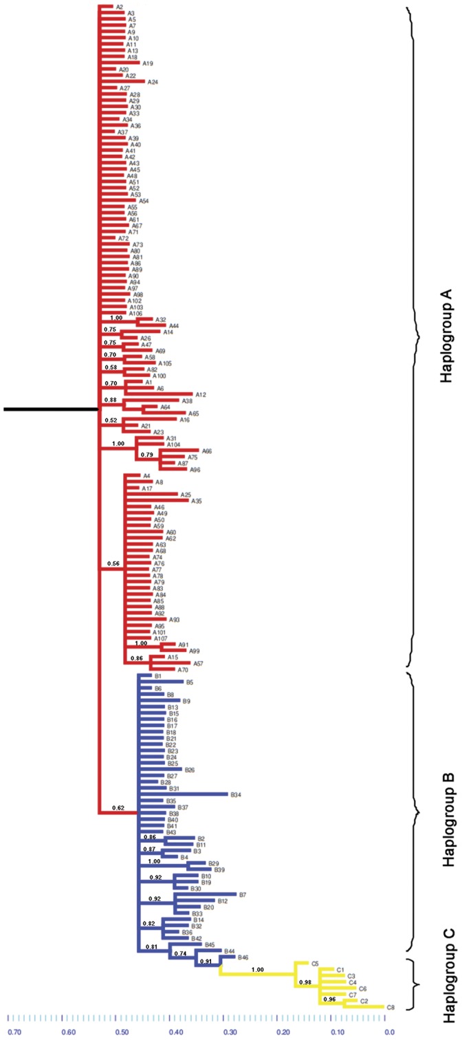
The tree is rooted using Strongylocentrotus purpuratus as outgroup (not shown); values for posterior probabilities >0.5, supporting non-collapsed clades, are indicated.

Population Structure

The analyses of population pairwise genetic differentiation (F _st and Jost’s D, Table 3) reflected a lack of population structure within both Eastern Atlantic and Mediterranean regions, but a clear differentiation between them and a complete differentiation (no alleles shared) of both regions from the Brazilian samples. Results from F _st and D were largely consistent. No significant differences could be found between any pair of localities from Cape Verde and Macaronesia, suggesting a high level of genetic flow among these Eastern Atlantic sub-regions. Likewise, no significant differences were found between any pair of Mediterranean localities (out of 136 possible pairs), with the exception of Torremuelle (the westernmost Mediterranean locality) where F _st analysis showed significant differences with two other Mediterranean localities, though these differences were not significant when D measures were analysed. Between Eastern Atlantic and Mediterranean, however, 38 (D) and 31 (F _st) comparisons (out of 85) were significant. Remarkably, the localities of Carboneras (Western Mediterranean), Crete and Kos (Eastern Mediterranean) did not show any significant difference to any other Eastern Atlantic or Mediterranean population, despite the large geographical distances involved in the case of the two latter localities.

Table 3. Genetic differentiation between Arbacia lixula populations, F _st (below the diagonal) and Jost’s D (above the diagonal).

	Brazil		East Atlantic					Mediterranean
	ITA	CFR	BOA	GIG	TEN	FAI	PIC	TOR	HER	CAR	PAL	VIL	BEN	XAB	CLM	TOS	COL	FOR	CAB	SCA	POP	CRE	KOS	ROD
ITA		0.115	1 *	1 *	1 *	1 *	1 *	1 *	1 *	1 *	1 *	1 *	1 *	1 *	1 *	1 *	1 *	1 *	1 *	1 *	1 *	1 *	1 *	1 *
CFR	0.132*		1 *	1 *	1 *	1 *	1 *	1 *	1 *	1 *	1 *	1 *	1 *	1 *	1 *	1 *	1 *	1 *	1 *	1 *	1 *	1 *	1 *	1 *
BOA	0.876 *	0.740 *		0.170	0.012	0.064	0.413	0.671 *	0.763*	0.275	0.553 *	0.598 *	0.557 *	0.656 *	0.225	0.889 *	0.751 *	0.664 *	0.510	0.632 *	0.608 *	0.181	0.270	0.715 *
GIG	0.865 *	0.712 *	0.030		0.039	0.024	0.215	0.445	0.555*	0.129	0.343	0.380	0.290	0.427	0.093	0.720*	0.669 *	0.512*	0.252	0.443	0.407	0.203	0.096	0.500*
TEN	0.825 *	0.676 *	0.015	0.002		0	0.037	0.662 *	0.499*	0.216	0.431	0.524*	0.454 *	0.453*	0.081	0.677*	0.448	0.453*	0.444	0.382	0.295	0.142	0.087	0.522*
FAI	0.861 *	0.719 *	0.007	0.022	0.000		0.038	0.670 *	0.623*	0.226	0.482 *	0.531 *	0.500 *	0.559 *	0.185	0.772 *	0.608 *	0.544 *	0.496	0.510 *	0.495 *	0.130	0.197	0.605 *
PIC	0.832 *	0.679 *	0.035	0.010	−0.006	0.013		0.501 *	0.150	0.214	0.226	0.309	0.272	0.178	0.081	0.230	0.097	0.102	0.326	0.092	0.067	0.124	0.040	0.146
TOR	0.830 *	0.674 *	0.228 *	0.136*	0.143 *	0.222 *	0.135 *		0.164	0.015	0	0	0	0.015	0.150	0.205	0.430	0.121	0	0.187	0.187	0.153	0.216	0.064
HER	0.833 *	0.687 *	0.053	0.043	0.002	0.043	0.001	0.113*		0.084	0	0	0.018	0	0.103	0	0	0	0.122	0	0	0.136	0.121	0
CAR	0.846 *	0.697 *	0.063	0.015	0.019	0.056	0.017	0.053	0.002		0	0	0	0	0	0.241	0.322	0.059	0	0.071	0.073	0	0	0.045
PAL	0.820 *	0.670 *	0.101 *	0.047	0.039	0.092 *	0.028	0.024	0.003	−0.014		0	0	0	0	0.008	0.118	0	0	0	0	0.020	0.013	0
VIL	0.810 *	0.662 *	0.100 *	0.038	0.043	0.095 *	0.036	0.015	0.013	−0.017	−0.020		0	0	0.037	0.074	0.227	0	0	0.019	0.042	0	0.110	0
BEN	0.849 *	0.701 *	0.177 *	0.090	0.097 *	0.172 *	0.083	−0.010	0.061	0.011	−0.006	−0.012		0	0	0.083	0.231	0	0	0.010	0.039	0.082	0.015	0
XAB	0.814 *	0.659 *	0.148 *	0.072	0.075	0.142 *	0.061	−0.006	0.039	0.002	−0.012	−0.020	−0.020		0.030	0	0.089	0	0	0	0	0	0.074	0
CLM	0.822 *	0.667 *	0.093*	0.057	0.027	0.084*	0.019	0.051	−0.012	−0.002	−0.019	−0.011	0.015	0.003		0.224	0.201	0.022	0	0.011	0.022	0	0	0.045
TOS	0.805 *	0.659 *	0.123 *	0.077	0.051	0.115 *	0.035	0.028	0.008	0.005	−0.018	−0.007	−0.000	−0.007	−0.021		0	0	0.174	0	0	0.269	0.194	0
COL	0.831 *	0.682 *	0.092 *	0.084 *	0.025	0.077 *	0.020	0.113*	−0.020	0.024	0.005	0.025	0.073	0.046	−0.017	0.001		0	0.338	0	0	0.236	0.175	0.009
FOR	0.829 *	0.681 *	0.085 *	0.053	0.020	0.074 *	0.013	0.065	−0.018	−0.009	−0.019	−0.006	0.024	0.010	−0.026	−0.017	−0.020		0.062	0	0	0.054	0.047	0
CAB	0.858 *	0.676 *	0.099*	0.037	0.026	0.088*	0.020	0.022	−0.001	−0.023	−0.028	−0.029	−0.015	−0.022	−0.029	−0.022	0.010	−0.023		0.051	0.093	0.069	0.001	0.003
SCA	0.819 *	0.651 *	0.122 *	0.069	0.044	0.111 *	0.026	0.037	0.002	0.002	−0.018	−0.007	0.006	−0.014	−0.022	−0.020	0.000	−0.017	−0.025		0	0.101	0	0
POP	0.826 *	0.680 *	0.096 *	0.067	0.027	0.087 *	0.018	0.063	−0.014	0.001	−0.014	0.000	0.028	0.011	−0.023	−0.021	−0.019	−0.020	−0.015	−0.017		0.105	0	0
CRE	0.833 *	0.693 *	0.037	0.016	0.003	0.030	0.004	0.088	−0.008	−0.011	0.001	0.002	0.047	0.027	−0.003	0.016	0.007	−0.005	−0.014	0.014	−0.001		0	0.105
KOS	0.833 *	0.686 *	0.064	0.025	0.013	0.058	0.005	0.053	−0.004	−0.016	−0.013	−0.008	0.013	0.007	−0.016	−0.011	0.008	−0.014	−0.029	−0.005	−0.016	−0.019		0.047
ROD	0.817 *	0.666 *	0.100 *	0.055	0.034	0.091 *	0.014	0.037	−0.004	−0.008	−0.021	−0.011	0.003	−0.009	−0.023	−0.024	−0.004	−0.023	−0.026	−0.024	−0.023	−0.000	−0.020

Consistently significant differences obtained by both methods after false discovery rate correction are represented in bold.

Significant P values for F _st obtained from randomization. *: significant after false discovery rate correction (P<0.0085).

Significant P values for D indicate that confidence interval obtained by bootstrapping excludes 0.

^*: significant after false discovery rate correction (P<0.0085).

The MDS analysis (Fig. 4) graphically expresses the relationships among populations obtained from F _st measures. Brazilian localities are widely separated in the first dimension from Eastern Atlantic and Mediterranean populations, whereas the Mediterranean and Eastern Atlantic populations were separated along the second axis. The lack of structure between sub-regions within the Eastern Atlantic and the Mediterranean is also apparent in the graphical arrangement. The same analysis using D measures (not shown) reflected the same overall structure.

Figure 4. Multidimensional scaling (MDS) for F _st differentiation of Arbacia lixula COI haplotypes.

Filled squares (▪) represent Brazilian populations, whereas filled circles (•) represent Eastern Atlantic populations and open circles (○) correspond to Mediterranean populations.

Consistent with the pairwise differentiation analysis, the AMOVA found significant differences between the three regions (Table 4), which remained significant when only Eastern Atlantic vs. Mediterranean regions were compared (Table 5). Conversely, and again in agreement with the pairwise differentiation analyses, no significant differences within regions between Eastern Atlantic sub-regions (Table 6) or among the three Mediterranean sub-basins (Table 7) were detected by AMOVA. The same results were obtained when these AMOVAs were repeated considering genetic distances between haplotypes (data not shown).

Table 4. Analysis of molecular variance (AMOVA) among regions using COI haplotype frequencies. Brazil vs. East Atlantic vs. Mediterranean.

Source of variation	df	Sum of squares	Variance components	Variation %	P value	Fixation index
Among groups	2	12.530	0.04690	9.69	<0.0001***	0.09692
Among populations within groups	21	9.728	0.00107	0.22	0.2583	0.00245
Within populations	580	252.833	0.43592	90.09	<0.0001***	0.09913
Total	603	275.091	0.48389

Table 5. Analysis of molecular variance (AMOVA) among regions using COI haplotype frequencies. East Atlantic vs. Mediterranean.

Source of variation	df	Sum of squares	Variance components	Variation %	P value	Fixation index
Between groups	1	4.104	0.01893	4.08	<0.0001***	0.04081
Among populations within groups	20	9.075	0.00035	0.08	0.3916	0.00080
Within populations	547	243.200	0.44461	95.84	0.0002***	0.04157
Total	568	256.380	0.46389

Table 6. Analysis of molecular variance (AMOVA) among sub-regions within Eastern Atlantic region, using COI haplotype frequencies: Macaronesia vs. Cape Verde.

Source of variation	df	Sum of squares	Variance components	Variation %	P value	Fixation index
Among groups	1	0.681	0.00483	1.04	0.400	0.01042
Among populations within groups	3	1.427	0.00074	0.16	0.385	0.00161
Within populations	118	54.046	0.45802	98.80	0.179	0.01201
Total	122	56.154	0.46359

Table 7. Analysis of molecular variance (AMOVA) among sub-regions within the Mediterranean, using COI haplotype frequencies: Alboran vs. Western Mediterranean vs. Eastern Mediterranean.

Source of variation	df	Sum of squares	Variance components	Variation %	P value	Fixation index
Between groups	2	0.829	−0.00023	−0.05	0.495	−0.00052
Among populations within groups	14	6.138	−0.00009	−0.02	0.482	−0.00021
Within populations	429	189.154	0.44092	100.07	0.514	−0.00073
Total	445	196.121	0.44059

The Mantel test showed significant isolation by distance when the whole dataset was analyzed (Fig. 5A). This result remained significant when populations from Brazil were excluded (Fig. 5B). Contrarily, no significant correlation between genetic differentiation and geographical distance was found when populations within just one region, either East Atlantic or Mediterranean, were analyzed (Fig. 5C & 5D).

Figure 5. Relationships between genetic and geographic distances for different datasets of Arbacia lixula populations.

Results of the Mantel test for isolation by distance are indicated.

Historical Demography

The mismatch distribution of Arbacia lixula populations from the Brazilian region (Fig. 6A) did not fit the sudden expansion model (Table 8). Conversely, the mismatch distribution for the Eastern Atlantic region (Fig. 6B) was remarkably unimodal. This indicates that a recent demographic expansion has occurred in this population. Similar results were obtained when only the Macaronesian sub-region was analyzed (Table 8). However, the distribution for the Cape Verde sub-basin did not fit the sudden expansion model, as reflected by a high SSD (Table 8). Nevertheless, this result may be an artefact due to small sample size (n = 27). The demographic expansion in the Eastern Atlantic populations could be dated, from the value of τ and the known mutation rate for the COI of Echinoidea, between 30.6–66.9 kya (thousand years ago), which is a surprisingly recent time.

Figure 6. Mismatch distributions of Arbacia lixula populations in the three studied regions.

Observed data and theoretical expected distributions are represented by discontinuous and solid lines, respectively. For Brazil (A), the theoretical expected distribution shown is that of a population of constant size. In the case of the East Atlantic (B) and the Mediterranean (C), data were fitted to a sudden expansion model.

Table 8. Mismatch distribution parameters for Arbacia lixula populations.

Region	SSD	τ	θ0	θ1	Estimated expansion time (kya)
Brazil	0.3525 **	N.A.	N.A.	N.A.	N.A.
Cape Verde	0.0265 *	N.A.	N.A.	N.A.	N.A.
Macaronesia	0.0004 ns	1.39	1.850	1000	31.3–68.4
Pooled East Atlantic	0.0014 ns	1.36	1.286	1000	30.6–66.9
Alboran Sea	0.0067 ns	4.24	0.000	12.54	95.4–208.7
West Mediterranean	0.0028 ns	4.20	0.000	9.75	94.5–206.7
East Mediterranean	0.0024 ns	3.90	0.001	10.86	87.7–191.9
Pooled Mediterranean	0.0026 ns	4.17	0.000	10.20	93.8–205.2
Whole Dataset	0.0030 ns	2.91	1.376	13.13	65.5–143.2

SSD values and their significances are presented along with sudden expansion model parameters and estimated time for the expansion (where applicable), for the studied regions and sub-regions and for the whole dataset.

^*: Significant at P<0.05.

^**: Significant at P<0.01.

^ns: Not significant.

N.A.: Not applicable (sudden expansion model rejected).

The mismatch distribution obtained for the Mediterranean region (Fig. 6C) was also typically unimodal. The parameters of the theoretical curves calculated individually for each Mediterranean sub-basin had all similar values, comparable to those of the whole Mediterranean region (Table 8), reinforcing the idea that all the Mediterranean Arbacia lixula populations belong to the same genetic pool. The demographic expansion in the Mediterranean could be dated between 93.8–205.2 kya. This estimation is a little older than that obtained for the Eastern Atlantic expansion, but is still a recent time.

The neutrality and population expansion tests calculated for the different regions and sub-basins (Table 9) were largely coherent with the results inferred from the mismatch distributions. Tajima’s D detected significant differences from neutrality in all cases, except for Brazil and the Eastern Mediterranean sub-basin. Fu’s F _s test for demographic expansion was significant in all cases (though just marginally so in the case of Brazil). Ramos-Onsins & Rozas’ R ₂ was significant for all cases except the Eastern Mediterranean sub-basin, and the raggedness value r was consistent with unimodal distributions, except for Brazilian and Cape Verdean populations.

Table 9. Neutrality and population expansion tests for Arbacia lixula in the studied regions or sub-regions and for the whole dataset.

Region	N	D	Fs	R 2	r
Brazil	35	−1.80405 ns	−3.712 *	0.0566 **	0.0503 *
Cape Verde	27	−2.08319 *	−9.809 ***	0.0527 ***	0.1254 *
Macaronesia	96	−2.40571 **	−45.988 ***	0.0234 ***	0.0167 ns
Pooled East Atlantic	123	−2.51677 ***	−70.825 ***	0.0185 ***	0.0265 ns
Alboran Sea	53	−1.83549 *	−15.648 ***	0.0421 **	0.0221 ns
West Mediterranean	310	−2.25417 **	−98.101 ***	0.0187 **	0.0137 ns
East Mediterranean	83	−1.49411 ns	−17.677 ***	0.0494 ns	0.0160 ns
Pooled Mediterranean	446	−2.28043 **	−155.806 ***	0.0162 ***	0.0137 ns
Whole Dataset	604	−2.32451 **	−256.026 ***	0.0150 **	0.0094 ns

Tajima’s D, Fu’s F_s statistic, Ramos-Onsins & Rozas’ statistic (R ₂), and raggedness index (r).

^*: Significant at P<0.05;

^**: Significant at P<0.01;

^***: Significant at P<0.001;

^ns: Not significant.

Discussion

COI and other mitochondrial markers have proven to be the most useful tool for tracing both intraspecific and intrageneric genealogies of many echinoid species [26], [64]–[65], [70]–[73] and usually yield easily interpretable results which are consistent with those of other nuclear markers. Nevertheless, our analyses are based on a single mitochondrial marker (COI). Thus, these results must be taken with caution, and further analyses using nuclear markers would be desirable. On the other hand, previous works in Echinoidea have shown that other nuclear markers were mainly used only to confirm the evolutionary history depicted by mtDNA [26], [72] or else displayed too much diversity to produce interpretable results [73].

The Arbacia lixula populations sampled showed high values of haplotype diversity and haplotype richness, but relatively low values of nucleotide diversity. The lowest diversity was found in Brazilian populations and, specifically, in the westernmost locality (Itaipu), which is close to the distribution limit of the species and separated from the other Brazilian locality by the Cabo Frio upwelling. In contrast, the highest diversity was found in the East Atlantic, as expected if this region is the geographical origin of the species [16], [26]. We detected three haplogroups in A. lixula. One of them (Group A) seems to be ancestral and is found only in Eastern Atlantic and Mediterranean populations, while another (Group B) is present at both sides of the Atlantic. The third one (Group C) is derived from Group B and found only in Brazil.

In a recent work, Lessios et al. [26] concluded that Arbacia lixula split from a common ancestor with A. punctulata ca. 2.6 Mya, and attributed this split to the mid-Atlantic barrier, separating the western A. punctulata from the eastern A. lixula, which would later have crossed back this barrier to establish itself, as an isolated clade, in the coast of Brazil. A problem with this view is that the mid-Atlantic barrier was fully in place long before the estimated date of the split, so the separation of the two species could not be a vicariance event but a range expansion event (on the part of the lineage that would become A. lixula), and two crossings of the barrier are required to fully explain the present-day distribution of the species (though the second crossing could be facilitated by the South Equatorial Current system [74]). An alternative scenario would be that the two Atlantic species diverged in Western Atlantic, after the rise of the Panama isthmus isolated their ancestor from the eastern Pacific region (the possible origin of the genus Arbacia [26]), and that A. lixula crossed the Atlantic ridge only once to colonize the Eastern Atlantic. Our results favour the first (Lessios’) view, as the haplotypes from Brazil formed a derived monophyletic group nested within the amphi-Atlantic Group B, rather than the opposite. This indicates a derived lineage in Western Atlantic, old enough to have had time to evolve forming the haplotype Group C. A more thorough sampling of the whole range of the Western Atlantic distribution and the inclusion of more data from Western Africa, are necessary before firm evidence can be obtained about the historical whereabouts of the main lineages of A. lixula.

Overall, the pattern of distribution of genetic variability (as shown in F _st, Jost’s D, MDS and AMOVA analyses) showed three groups of populations that differed significantly from each other (Brazilian, Eastern Atlantic and Mediterranean), while little structure could be found within these groups. It is remarkable that the F _st measures based on sequence distance metrics and the differentiation measure D based on haplotype frequencies yielded essentially the same results. This is attributable to the prevalence of close haplotypes separated by small number of mutations (hence the low nucleotide diversity in general) that are widespread among populations. Thus, haplotype genetic differences had relatively little weight and most population structure derives from haplotype frequency differences.

Another striking pattern resulting from our molecular analyses is that recent demographic phenomena have shaped the present-day genetic structure of Arbacia lixula populations in the Eastern Atlantic and the Mediterranean. This does not seem to be the case of the Brazilian population but, given the small sample size, it is unclear if the resulting mismatch distribution (Fig. 6A) is either multimodal or L-shaped in this population. Multimodal curves are typical of populations at demographic equilibrium, but L-shaped distributions may result from very recent demographic bottlenecks [75]. More extensive sampling would be required to get the full picture of the demographic processes that have shaped the Brazilian populations of A. lixula.

The lack of an exclusively Mediterranean mitochondrial lineage of Arbacia lixula is remarkable. Other Atlanto-Mediterranean echinoderms such as Marthasterias glacialis [76], Holothuria mammata [77] or Paracentrotus lividus [73], [78] do have lineages exclusive of the Mediterranean. These species have been probably present in the Mediterranean for several million years and their populations may have suffered several episodes of impaired gene flow during the Pleistocene glaciations. The genetic structure shown by A. lixula probably reflects a different demographic history from these other species.

Even if there is no phylogenetic break in the Mediterranean (as also found by Lessios et al. [26]) and alleles are widely shared at both sides of the Gibraltar boundary, this barrier seems nevertheless to restrict gene flow in Arbacia lixula, so as to establish significant differences in terms of haplotype frequencies between Mediterranean and Eastern Atlantic populations. The AMOVA (and pairwise comparisons) detected significant genetic differentiation between these groups of populations (Table 5), suggesting a reduced gene flow through the Strait of Gibraltar. Differently to what can be found in other marine organisms [79], the Strait itself, and not the Almeria-Oran Front (some 350 Km east of Gibraltar), is the place of the phylogeographic break, as the populations from the Alboran Sea are undistinguishable from other Mediterranean populations, but are significantly differentiated from most Atlantic populations (Fig. 4, Tables 3 and 7). Thus, A. lixula does not show any genetic differentiation among populations throughout the whole Mediterranean Sea. This could be due to recurrent gene flow, but oceanographic barriers such as the Almeria-Oran Front or the Siculo-Tunisian Strait [79] are strong enough to maintain genetic differentiation among different sub-basins in the case of other echinoderms of similar larval dispersive capacity [73], [77]–[78]. We favour the alternative explanation (for the lack of genetic structure) that the colonization of the Mediterranean by A. lixula is so recent (see below) that populations in the different Mediterranean sub-basins have not had yet enough time to diverge from each other.

In the case of Macaronesian and Cape Verdean populations (Table 6), it seems likely that the present-day genetic similarity could be the result of a recent demographic expansion (see below), which could have swamped any trace of previous differentiated lineages potentially formed during periods of restricted gene flow among archipelagos.

Brazilian populations of Arbacia lixula are completely differentiated from Eastern Atlantic and Mediterranean populations (Tables 3 & 4). In addition, they showed the lowest genetic diversity and did not show any signature of demographic expansion. Nevertheless, our sample size is small, and Northern and Central Brazilian populations of A. lixula have never been sampled for phylogeographic studies. More extensive sampling along the Brazilian coast would be required for a full understanding of factors shaping the genetic structure of the West Atlantic populations of A. lixula.

The almost complete lack of fossil record for Arbacia lixula in the Mediterranean is most revealing. At present, the species is highly abundant and occurs in areas that have been thoroughly sampled by palaeontologists. Other Mediterranean echinoids currently co-occurring in the same habitats are commonly found in assemblages of the Pleistocene and have been abundantly reported in the paleontological literature [80]–[83]. In contrast, only one fossil individual of A. lixula from the Mediterranean has ever been reported in the literature [13]. It was found in very young deposits from Livorno (Italy) whose recency led Stefanini to speculate that A. lixula had an exotic origin and had entered the Mediterranean in recent times [13]. A. lixula is consistently absent from fossil assemblages of the so-called “Senegalese fauna” that characterize the warmer periods from the Tyrrhenian stage (ca. 260–11.4 kya), which have been extensively sampled and thoroughly described [84]–[89].

As for the Atlantic archipelagos, recent work on the fossil echinoid fauna of Azores Islands [90] has revealed the presence of A. lixula, providing several tens of pieces of individuals, including the oldest known record of this species. These deposits are currently dated to 130–120 kya [91], which corresponds to the last interglacial or Riss-Würm (also called MIS 5e, ca. 130–114 kya). These specimens add up to the only other Atlantic A. lixula fossil specimen known from the Pleistocene of Madeira [13] whose dating is more uncertain.

Thus, there is scarce paleontological evidence of the occurrence of Arbacia lixula in the Mediterranean, and somewhat more, but still scarce, evidence of the colonization of the Atlantic archipelagos of Azores and Madeira, which probably occurred during the last interglacial period of the Pleistocene (MIS 5e). These observations are in agreement with the genetic signatures we observed in the mismatch distributions, which clearly show that recent sudden expansions have occurred in the Mediterranean and Macaronesian populations (Fig. 6). This is also supported by the strikingly star-shaped topologies of the haplotype network (Fig. 2) and by the comb-like clades in the BI phylogenetic tree (Fig. 3). Our temporal estimation for the demographic expansion in the Mediterranean (93.8–205.2 kya) is coherent with the only available fossil record [13]. This is considerably younger than the times for expansion events found in other Mediterranean echinoderms using the same estimation method, which vary from 300 to 600 kya [73], [77] and fits with the possibility that the colonization of the Mediterranean by A. lixula took place as recently as during the last interglacial period (MIS 5e). This period was also the longest of all interglacial warm periods of the Pleistocene. The minimum winter surface temperature of the Mediterranean Sea stayed warmer than 19°C for several thousands of years [89]. This probably enabled tropical Atlantic populations of A. lixula to cross the Strait of Gibraltar and colonize the Mediterranean.

In the case of Eastern Atlantic populations, the exponential demographic expansion is even more apparent, since the mismatch distribution follows a sharp unimodal curve which fits to a sudden expansion model with a very high value for θ₁. This expansion probably occurred more recently than in the Mediterranean (31.3–68.4 kya). This estimation falls within the Late Pleistocene, an epoch generally dominated by the last glaciation (Würm), during which the mean sea level dropped down to 80 m below the present level [92]–[93]. Changes in ocean circulation related to this sea level drop can be related to the population expansion of A. lixula in the Eastern Atlantic. Contrary to what happens in the Mediterranean, the fossils available show that the species was present in Macaronesia before this expansion [90], so the demographic history of the Atlantic populations of A. lixula seems to be more complex than that of the Mediterranean populations. To complete the picture of the colonization of Atlantic archipelagos, data from continental African shores would be highly valuable.

An invasive species can be defined as a “species that threatens the diversity or abundance of native species, the ecological stability of infested ecosystems, economic activities (e.g., agricultural, aquacultural, commercial, or recreational) dependent on these ecosystems and/or human health” [94]. Although the term is generally applied to species introduced as a result of human activities, it should not be necessarily so. Moreover, ecosystem engineer species such as Arbacia lixula, that have shaped contemporary communities as the result of a colonization event that took place many years ago, can be falsely viewed as native [95]. According to our molecular data, A. lixula has indeed colonized the Mediterranean recently and complies with the terms of the former definition, even if it is usually viewed as native because its colonization took place following natural climatic changes, without human intervention.

Whether considered as an “old natural invader” or as native, the present trend of global warming can potentially boost the negative impact of A. lixula in Mediterranean ecosystems, thus possibly turning a “natural” colonization into an ecological problem related (at least partially) to human intervention. The ongoing warming [96] may facilitate population blooms of A. lixula in Northern Mediterranean, by releasing the constraint to larval development due to low water temperature. Warnings have been issued about its potential population increase and the generation of barren grounds in sublittoral habitats [10]–[11].

Thus, genetic data are in agreement with the consideration of Arbacia lixula as a thermophilous species that has recently colonised the Mediterranean and whose densities may increase in the foreseeable future. Monitoring of populations seems highly recommendable as a management tool in the near future for protecting the threatened Mediterranean shallow water ecosystems.

Supporting Information

Table S1

Haplotype frequencies of Arbacia lixula COI for all sampled localities. Haplotypes shared by two or more localities are represented in bold, while numbers not in bold correspond to private haplotypes. Background colours correspond to the three different haplogroups. Outgroups weights calculated by tcs are also displayed for each haplotype, and that with the highest outgroup weight (A2) is highlighted in green background.

(XLS)

Funding Statement

This work was funded by projects CTM2010-22218 from the Spanish Government, 2009SGR-484 from the Catalan Government, BIOCON 08-187/09 from BBVA Foundation and 287844 (COCONET) of the European Community’s Seventh Framework Programme (FP7/2007–2013). RPP is supported in part by a “Juan de la Cierva” contract (Ministry of Science and Technology, Spanish Government). The funders had no role in the study design, data collection and analysis, decision to publish, or preparation of the manuscript.

References

- 1. Palacín C, Turon X, Ballesteros M, Giribet G, López S (1998) Stock evaluation of three littoral echinoid species on the Catalan coast (North-Western Mediterranean). Marine Ecology 19: 163–177 doi:10.1111/j.1439-0485.1998.tb00460.x. [Google Scholar]
- 2. Sala E, Boudouresque CF, Harmelin-Vivien ML (1998) Fishing, trophic cascades, and the structure of algal assemblages: evaluation of an old but untested paradigm. Oikos 82: 425–439. [Google Scholar]
- 3. Palacín C, Giribet G, Carner S, Dantart L, Turon X (1998) Low densities of sea urchins influence the structure of algal assemblages in the western Mediterranean. Journal of Sea Research 39: 281–290 doi:10.1016/S1385-1101(97)00061-0. [Google Scholar]
- 4. Bulleri F, Benedetti-Cecchi L, Cinelli F (1999) Grazing by the sea urchins Arbacia lixula L. and Paracentrotus lividus Lam. in the Northwest Mediterranean. Journal of Experimental Marine Biology and Ecology 241: 81–95 doi:10.1016/S0022–0981(99)00073-8. [DOI] [PubMed] [Google Scholar]
- 5. Wangensteen OS, Turon X, García-Cisneros A, Recasens M, Romero J, et al. (2011) A wolf in sheep’s clothing: carnivory in dominant sea urchins in the Mediterranean. Marine Ecology Progress Series 441: 117–128 doi:10.3354/meps09359. [Google Scholar]
- 6.Verlaque M (1987) Relations entre Paracentrotus lividus (Lamarck) et le phytobenthos de Méditerranée occidentale. In: Colloque International Sur Paracentrotus lividus et les Oursins Comestibles. Marseille: GIS Posidonie Publ. 5–36.
- 7.Hereu B (2004) The role of trophic interactions between fishes, sea urchins and algae in the northwestern Mediterranean rocky infralittoral. PhD thesis, University of Barcelona.
- 8. Bulleri F, Bertocci I, Micheli F (2002) Interplay of encrusting coralline algae and sea urchins in maintaining alternative habitats. Marine Ecology Progress Series 243: 101–109 doi:10.3354/meps243101. [Google Scholar]
- 9. Privitera D, Chiantore M, Mangialajo L, Glavic N, Kozul W, et al. (2008) Inter- and intra-specific competition between Paracentrotus lividus and Arbacia lixula in resource-limited barren areas. Journal of Sea Research 60: 184–192 doi:10.1016/j.seares.2008.07.001. [Google Scholar]
- 10. Gianguzza P, Agnetta D, Bonaviri C, Di Trapani F, Visconti G, et al. (2011) The rise of thermophilic sea urchins and the expansion of barren grounds in the Mediterranean Sea. Chemistry and Ecology 27: 129–134 doi:10.1080/02757540.2010.547484. [Google Scholar]
- 11. Privitera D, Noli M, Falugi C, Chiantore M (2011) Benthic assemblages and temperature effects on Paracentrotus lividus and Arbacia lixula larvae and settlement. Journal of Experimental Marine Biology and Ecology 407: 6–11 doi:10.1016/j.jembe.2011.06.030. [Google Scholar]
- 12.Riedl R (1983) Fauna und Flora des Mittelmeeres. Hamburg & Berlin: Verlag Paul Parey. 836 p.
- 13. Stefanini G (1911) Di alcune Arbacia fossili. Rivista Italiana di Paleontologia 17: 51–52. [Google Scholar]
- 14.Mortensen T (1935) A monograph of the Echinoidea. II. Bothriocidaroida, Melonechinoida, lepidocentroida, and Stirodonta. Copenhagen & London: Reitzel & Oxford Univ. Press. 647 p.
- 15. Kempf M (1962) Recherches d´écologie comparée sur Paracentrotus lividus (Lmk.) et Arbacia lixula (L.). Recueil des Travaux de la Station Marine d’Endoume 25: 47–116. [Google Scholar]
- 16.Tortonese E (1965) Echinodermata. Fauna d’Italia vol. VI. Bologna: Calderini. 422 p.
- 17. Fenaux L (1968) Maturation des gonades et cycle saisonnier des larves chez A. lixula, P. lividus et P. microtuberculatus à Villefranche-Sur-Mer. Vie et Milieu Série A Biologie Marine 19: 1–52. [Google Scholar]
- 18. Petit G, Delamare-Deboutteville C, Bougis P (1950) Le fichier faunistique du laboratoire Arago. Vie et Milieu Série A Biologie Marine 1: 356–360. [Google Scholar]
- 19. Marion AF (1883) Esquisse d’une topographie zoologique du Golfe de Marseille. Annales du Musée d’Histoire Naturelle de Marseille, Zoologie 1: 6–108. [Google Scholar]
- 20. Francour P, Boudouresque CF, Harmelin JG, Harmelin-Vivien ML, Quignard JP (1994) Are the Mediterranean waters becoming warmer? Information from biological indicators. Marine Pollution Bulletin 28: 523–526. [Google Scholar]
- 21.Harmelin JG, Hereu B, de Maisonnave LM, Teixidor N, Domínguez L, et al.. (1995) Indicateurs de biodiversité en milieu marin: les échinodermes. Fluctuations temporelles des peuplements d’échinodermes à Port-Cros. Comparaison entre les années 1982–84 et 1993–95.
- 22. Kroh A, Smith AB (2010) The phylogeny and classification of post-Palaeozoic echinoids. Journal of Systematic Palaeontology 8: 147–212 doi:10.1080/14772011003603556. [Google Scholar]
- 23. Hart MW (2012) New sea urchin phylogeography reveals latitudinal shifts associated with speciation. Molecular Ecology 21: 26–27 doi:10.1111/j.1365-294X.2011.05375.x. [DOI] [PubMed] [Google Scholar]
- 24. Metz EC, Gómez-Gutiérrez G, Vacquier VD (1998) Mitochondrial DNA and bindin gene sequence evolution among allopatric species of the sea urchin genus Arbacia . Molecular Biology and Evolution 15: 185–195. [DOI] [PubMed] [Google Scholar]
- 25. Martins CS, Hamann M, Fiúza AFG (2002) Surface circulation in the eastern North Atlantic, from drifters and altimetry. Journal of Geophysical Research C Oceans 107: 3217–3238 doi:10.1029/2000JC000345. [Google Scholar]
- 26. Lessios HA, Lockhart S, Collin R, Sotil G, Sánchez-Jérez P, et al. (2012) Phylogeography and bindin evolution in Arbacia, a sea urchin genus with an unusual distribution. Molecular Ecology 21: 130–144 doi: 10.1111/j.1365-294X.2011.05303.x. [DOI] [PubMed] [Google Scholar]
- 27. De Giorgi C, Martiradonna A, Lanave C, Saccone C (1996) Complete sequence of the mitochondrial DNA in the sea urchin Arbacia lixula: conserved features of the echinoid mitochondrial genome. Molecular Phylogenetics and Evolution 5: 323–332 doi:10.1006/mpev.1996.0027. [DOI] [PubMed] [Google Scholar]
- 28. Rozen S, Skaletsky H (2000) Primer3 on the WWW for general users and for biologist programmers. In: Misener S, Krawetz SA, editors. Bioinformatics Methods and Protocols. New Jersey: Humana Press, Vol. 132: 365–386 doi:10.1385/1592591922. [DOI] [PubMed] [Google Scholar]
- 29. Hall TA (1999) BioEdit: a user-friendly biological sequence alignment editor and analysis program for Windows 95/98/NT. Nucleic Acids Symposium Series 41: 95–98. [Google Scholar]
- 30. Tamura K, Peterson D, Peterson N, Stecher G, Nei M, et al. (2011) MEGA5: Molecular evolutionary genetics analysis using maximum likelihood, evolutionary distance, and maximum parsimony methods. Molecular Biology and Evolution 28: 2731–2739 doi:10.1093/molbev/msr121. [DOI] [PMC free article] [PubMed] [Google Scholar]
- 31. Nei M, Gojobori T (1986) Simple methods for estimating the numbers of synonymous and nonsynonymous nucleotide substitutions. Mol Biol Evol 3: 418–426. [DOI] [PubMed] [Google Scholar]
- 32. Jukes TH, Cantor CR (1969) Evolution of protein molecules. In: Munro HN, editor. Mammalian Protein Metabolism III. New York: Academic Press, Vol. III: 21–132. [Google Scholar]
- 33. Librado P, Rozas J (2009) DnaSP v5: a software for comprehensive analysis of DNA polymorphism data. Bioinformatics 25: 1451–1452 doi:10.1093/bioinformatics/btp187. [DOI] [PubMed] [Google Scholar]
- 34. Petit RJ, El Mousadik A, Pons O (2008) Identifying populations for conservation on the basis of genetic markers. Conservation Biology 12: 844–855 doi:10.1111/j.1523-1739.1998.96489.x. [Google Scholar]
- 35. Corander J, Marttinen P, Sirén J, Tang J (2008) Enhanced Bayesian modelling in BAPS software for learning genetic structures of populations. BMC Bioinformatics 9: 539 doi:10.1186/1471-2105-9-539. [DOI] [PMC free article] [PubMed] [Google Scholar]
- 36. Corander J, Tang J (2007) Bayesian analysis of population structure based on linked molecular information. Mathematical Biosciences 205: 19–31 doi:10.1016/j.mbs.2006.09.015. [DOI] [PubMed] [Google Scholar]
- 37. Bandelt H, Forster P, Rohl A (1999) Median-joining networks for inferring intraspecific phylogenies. Molecular Biology and Evolution 16: 37–48. [DOI] [PubMed] [Google Scholar]
- 38. Templeton AR, Boerwinkle E, Sing CF (1987) A cladistic analysis of phenotypic associations with haplotypes inferred from restriction endonuclease mapping. I. Basic theory and an analysis of alcohol dehydrogenase activity in Drosophila. Genetics 117: 343–351. [DOI] [PMC free article] [PubMed] [Google Scholar]
- 39. Templeton AR, Sing CF (1993) A cladistic analysis of phenotypic associations with haplotypes inferred from restriction endonuclease mapping. IV. Nested analyses with cladogram uncertainty and recombination. Genetics 134: 659–669. [DOI] [PMC free article] [PubMed] [Google Scholar]
- 40. Castelloe J, Templeton AR (1994) Root probabilities for intraspecific gene trees under neutral coalescent theory. Molecular phylogenetics and evolution 3: 102–113 doi:10.1006/mpev.1994.1013. [DOI] [PubMed] [Google Scholar]
- 41. Clement M, Posada D, Crandall K a (2000) TCS: a computer program to estimate gene genealogies. Molecular ecology 9: 1657–1659. [DOI] [PubMed] [Google Scholar]
- 42. Jacobs HT, Elliott DJ, Math VB, Farquharson A (1988) Nucleotide sequence and gene organization of sea urchin mitochondrial DNA. Journal of Molecular Biology 202: 185–217 doi: 10.1016/0022-2836(88)90452-4. [DOI] [PubMed] [Google Scholar]
- 43.Crandall KA, Templeton AR, Sing CF (1994) Intraspecific phylogenetics, problems and solutions. In: Scotland RW, Siebert DJ, Williams DM, editors. Models in Phylogeny Reconstruction. Oxford: Clarendon Press. 273–297.
- 44. Posada D (2008) jModelTest: phylogenetic model averaging. Molecular Biology and Evolution 25: 1253–1256 doi:10.1093/molbev/msn083. [DOI] [PubMed] [Google Scholar]
- 45. Guindon S, Gascuel O (2003) A simple, fast, and accurate algorithm to estimate large phylogenies by maximum likelihood. Systematic Biology 52: 696–704 doi:10.1080/10635150390235520. [DOI] [PubMed] [Google Scholar]
- 46. Tamura K, Nei M (1993) Estimation of the number of nucleotide substitutions in the control region of mitochondrial DNA in humans and chimpanzees. Molecular Biology and Evolution 10: 512–526. [DOI] [PubMed] [Google Scholar]
- 47. Huelsenbeck JP, Ronquist F (2001) MRBAYES: Bayesian inference of phylogenetic trees. Bioinformatics 17: 754–755 doi:10.1093/bioinformatics/17.8.754. [DOI] [PubMed] [Google Scholar]
- 48.Maddison WP, Maddison DR (2011) MESQUITE: a modular system for evolutionary analysis website. Available: http://mesquiteproject.org. Accessed 2012 Apr 24.
- 49. Excoffier L, Laval G, Schneider S (2005) Arlequin (version 3.0): an integrated software package for population genetics data analysis. Evolutionary Bioinformatics Online 1: 47–50. [PMC free article] [PubMed] [Google Scholar]
- 50. Benjamini Y, Yekutieli D (2001) The control of the false discovery rate in multiple testing under dependency. Annals of Statistics 29: 1165–1188 doi:10.1214/aos/1013699998. [Google Scholar]
- 51. Narum SR (2006) Beyond Bonferroni: Less conservative analyses for conservation genetics. Conservation Genetics 7: 783–787 doi:10.1007/s10592-005-9056-y. [Google Scholar]
- 52.Cox TF, Cox MAA (1994) Multidimensional Scaling. London: Chapman & Hall. 213 p.
- 53. Racine JS (2012) RStudio: A Platform-Independent IDE for R and Sweave. Journal of Applied Econometrics 27: 167–172 doi:10.1002/jae.1278. [Google Scholar]
- 54. Jost L (2008) GST and its relatives do not measure differentiation. Molecular Ecology 17: 4015–4026 doi:10.1111/j.1365-294X.2008.03887.x. [DOI] [PubMed] [Google Scholar]
- 55.Chao A, Shen TJ (2010) Program SPADE (Species Prediction and Diversity Estimation). http://chao.stat.nthu.edu.tw/softwareCE.html.
- 56. Excoffier L, Smouse PE, Quattro JM (1992) Analysis of molecular variance inferred from metric distances among DNA haplotypes: application to human mitochondrial DNA restriction data. Genetics 131: 479–491. [DOI] [PMC free article] [PubMed] [Google Scholar]
- 57. Slatkin M (1995) A measure of population subdivision based on microsatellite allele frequencies. Genetics 139: 457–462. [DOI] [PMC free article] [PubMed] [Google Scholar]
- 58. Rousset F (1997) Genetic differentiation and estimation of gene flow from F-statistics under isolation by distance. Genetics 145: 1219–1228. [DOI] [PMC free article] [PubMed] [Google Scholar]
- 59. Rogers AR, Harpending HC (1992) Population growth makes waves in the distribution of pairwise genetic differences. Molecular Biology and Evolution 9: 552–569. [DOI] [PubMed] [Google Scholar]
- 60. Schneider S, Excoffier L (1999) Estimation of past demographic parameters from the distribution of pairwise differences when the mutation rates vary among sites: application to human mitochondrial DNA. Genetics 152: 1079–1089. [DOI] [PMC free article] [PubMed] [Google Scholar]
- 61. Rogers AR (1995) Genetic evidence for a Pleistocene population explosion. Evolution 49: 608–615. [DOI] [PubMed] [Google Scholar]
- 62. Watterson G (1975) On the number of segregating sites in genetical models without recombination. Theoretical Population Biology 7: 256–276. [DOI] [PubMed] [Google Scholar]
- 63. Slatkin M, Hudson RR (1991) Pairwise comparisons of mitochondrial DNA sequences in stable and exponentially growing populations. Genetics 129: 555–562. [DOI] [PMC free article] [PubMed] [Google Scholar]
- 64. Lessios HA, Kessing BD, Pearse JS (2001) Population structure and speciation in tropical seas: global phylogeography of the sea urchin Diadema . Evolution 55: 955–975 doi:10.1111/j.0014-3820.2001.tb00613.x. [DOI] [PubMed] [Google Scholar]
- 65. McCartney MA, Keller G, Lessios HA (2000) Dispersal barriers in tropical oceans and speciation in Atlantic and eastern Pacific sea urchins of the genus Echinometra. . Molecular Ecology 9: 1391–1400 doi:10.1046/j.1365-294x.2000.01022.x. [DOI] [PubMed] [Google Scholar]
- 66. Tajima F (1989) Statistical method for testing the neutral mutation hypothesis by DNA polymorphism. Genetics 123: 585–595. [DOI] [PMC free article] [PubMed] [Google Scholar]
- 67. Fu YX (1997) Statistical tests of neutrality of mutations against population growth, hitchhiking and background selection. Genetics 147: 915–925. [DOI] [PMC free article] [PubMed] [Google Scholar]
- 68. Ramos-Onsins SE, Rozas J (2002) Statistical properties of new neutrality tests against population growth. Molecular Biology and Evolution 19: 2092–2100. [DOI] [PubMed] [Google Scholar]
- 69. Harpending HC (1994) Signature of ancient population growth in a low-resolution mitochondrial DNA mismatch distribution. Human Biology 66: 591–600. [PubMed] [Google Scholar]
- 70. Lessios HA, Kessing BD, Robertson DR, Paulay G (1999) Phylogeography of the Pantropical Sea Urchin Eucidaris in Relation to Land Barriers and Ocean Currents. Evolution 53: 806–817. [DOI] [PubMed] [Google Scholar]
- 71. Lessios HA, Kane J, Robertson DR, Wallis G (2003) Phylogeography of the pantropical sea urchin Tripneustes: contrasting patterns of population structure between oceans. Evolution 57: 2026–2036. [DOI] [PubMed] [Google Scholar]
- 72. Zigler KS, Lessios HA (2004) Speciation on the coasts of the New World: Phylogeography and the evolution of bindin in the sea urchin genus Lytechinus . Evolution 58: 1225–1241 doi:10.1111/j.0014-3820.2004.tb01702.x. [DOI] [PubMed] [Google Scholar]
- 73. Calderón I, Giribet G, Turon X (2008) Two markers and one history: phylogeography of the edible common sea urchin Paracentrotus lividus in the Lusitanian region. Marine Biology 154: 137–151 doi:10.1007/s00227-008-0908-0. [Google Scholar]
- 74. Lumpkin R, Garzoli S (2005) Near-surface circulation in the Tropical Atlantic Ocean. Deep Sea Research Part I: Oceanographic Research Papers 52: 495–518 doi:10.1016/j.dsr.2004.09.001. [Google Scholar]
- 75. Marjoram P, Donnelly P (1994) Pairwise Comparisons of Mitochondrial DNA Sequences in Subdivided Populations and Implications for Early Human Evolution. Genetics 136: 673–683. [DOI] [PMC free article] [PubMed] [Google Scholar]
- 76. Pérez-Portela R, Villamor A, Almada VC (2010) Phylogeography of the sea star Marthasterias glacialis (Asteroidea, Echinodermata): deep genetic divergence between mitochondrial lineages in the north-western mediterranean. Marine Biology 157: 2015–2028 doi:10.1007/s00227-010-1470-0. [Google Scholar]
- 77. Borrero-Pérez GH, González-Wangüemert M, Marcos C, Pérez-Ruzafa A (2011) Phylogeography of the Atlanto-Mediterranean sea cucumber Holothuria (Holothuria) mammata: the combined effects of historical processes and current oceanographical pattern. Molecular Ecology 20: 1964–1975 doi:10.1111/j.1365-294X.2011.05068.x. [DOI] [PubMed] [Google Scholar]
- 78. Maltagliati F, Di Giuseppe G, Barbieri M, Castelli A, Dini F (2010) Phylogeography and genetic structure of the edible sea urchin Paracentrotus lividus (Echinodermata: Echinoidea) inferred from the mitochondrial cytochrome b gene. Biological Journal of the Linnean Society 100: 910–923 doi: 10.1111/j.1095–8312.2010.01482.x. [Google Scholar]
- 79. Patarnello T, Volckaert FAMJ, Castilho R (2007) Pillars of Hercules: is the Atlantic-Mediterranean transition a phylogeographical break? Molecular Ecology 16: 4426–4444 doi:10.1111/j.1365-294X.2007.03477.x. [DOI] [PubMed] [Google Scholar]
- 80. Cuerda J, Antich S, Soler A (1986) Las formaciones cuaternarias marinas de Cala Pí (Mallorca). Bolletí de la Societat d’Història Natural de les Balears 30: 95–104. [Google Scholar]
- 81. Villalba-Currás MP, Jordá-Pardo JF, Aura-Tortosa JE (2007) Los equínidos del Pleistoceno Superior y Holoceno del registro arqueológico de la Cueva de Nerja (Málaga, España). Cuaternario y Geomorfología 21: 133–148. [Google Scholar]
- 82. Néraudeau D, Masrour M (n.d.) Évolution de la biodiversité et de la distribution paléobiogéographique des échinides sur les côtes atlantiques du Maroc du Tortonien à l’Actuel. Geodiversitas 30: 211–232. [Google Scholar]
- 83. Scicchitano G, Spampinato CR, Ferranti L, Antonioli F, Monaco C, et al. (2011) Uplifted Holocene shorelines at Capo Milazzo (NE Sicily, Italy): Evidence of co-seismic and steady-state deformation. Quaternary International 232: 201–213 doi:10.1016/j.quaint.2010.06.028. [Google Scholar]
- 84. Cuerda J (1957) Fauna marina del Tirreniense de la bahía de Palma (Mallorca). Bolletí de la Societat d’Història Natural de les Balears 3: 3–75. [Google Scholar]
- 85. Hillaire-Marcel C, Carro O, Causse C, Goy JL, Zazo C (1986) Th/U dating of Strombus bubonius-bearing marine terraces in southeastern Spain. Geology 14: 613–616 doi:10.1130/0091-7613(1986)14<613:TDOSBM>2.0.CO;2. [Google Scholar]
- 86. Lillo-Carpio MJ (1988) Consideraciones sobre los afloramientos tirrenienses detectados entre Cabo Roig (Alicante) y la desembocadura del río Almanzora (Almería). Papeles de Geografia 14: 51–81. [Google Scholar]
- 87. Lario J, Zazo C, Somoza L, Goy JL, Hoyos M, et al. (1993) Los episodios marinos cuaternarios de la costa de Málaga (España). Revista de la Sociedad Geológica de España 6: 41–46. [Google Scholar]
- 88. Belluomini G, Caldara M, Casini C, Cerasoli M, Manfra L, et al. (2002) The age of Late Pleistocene shorelines and tectonic activity of Taranto area, Southern Italy. Quaternary Science Reviews 21: 525–547 doi:10.1016/S0277-3791(01)00097-X. [Google Scholar]
- 89. Bardaji T, Goy JL, Zazo C, Hillaire-Marcel C, Dabrio C, et al. (2009) Sea level and climate changes during OIS 5e in the Western Mediterranean. Geomorphology 104: 22–37 doi:10.1016/j.geomorph.2008.05.027. [Google Scholar]
- 90. Madeira P, Kroh A, Cordeiro R, Meireles R, Ávila SP (2011) The fossil echinoids of Santa Maria Island, Azores (Northern Atlantic Ocean). Acta Geologica Polonica 61: 243–264. [Google Scholar]
- 91. Ávila SP, Madeira P, Mendes N, Rebelo A, Medeiros A, et al. (2008) Mass extinctions in the Azores during the last glaciation: fact or myth? Journal of Biogeography 35: 1123–1129 doi:10.1111/j.1365-2699.2008.01881.x. [Google Scholar]
- 92. Guilcher A (1969) Pleistocene and Holocene sea level changes. Earth-Science Reviews 5: 69–97 doi:10.1016/0012-8252(69)90079-8. [Google Scholar]
- 93. Waelbroeck C, Labeyrie L, Michel E, Duplessy JC, McManus JF, et al. (2002) Sea-level and deep water temperature changes derived from benthic foraminifera isotopic records. Quaternary Science Reviews 21: 295–305 doi:10.1016/S0277-3791(01)00101-9. [Google Scholar]
- 94. Occhipinti-Ambrogi A, Galil BS (2004) A uniform terminology on bioinvasions: a chimera or an operative tool? Marine pollution bulletin 49: 688–694 doi:10.1016/j.marpolbul.2004.08.011. [DOI] [PubMed] [Google Scholar]
- 95. Haydar D (2012) What is natural? The scale of cryptogenesis in the North Atlantic Ocean. Diversity and Distributions 18: 101–110 doi:10.1111/j.1472-4642.2011.00863.x. [Google Scholar]
- 96. Burrows MT, Schoeman DS, Buckley LB, Moore P, Poloczanska ES, et al. (2011) The pace of shifting climate in marine and terrestrial ecosystems. Science 334: 652–655 doi:10.1126/science.1210288. [DOI] [PubMed] [Google Scholar]
Associated Data
This section collects any data citations, data availability statements, or supplementary materials included in this article.
Supplementary Materials