Analyzing protein-protein interactions from affinity purification-mass spectrometry data with SAINT

Abstract

Significance Analysis of INTeractome (SAINT) is a software package for scoring protein-protein interactions based on label-free quantitative proteomics data (e.g. spectral count or intensity) in affinity purification – mass spectrometry (AP-MS) experiments. SAINT allows bench scientists to select bona fide interactions and remove non-specific interactions in an unbiased manner. However, there is no `one-size-fits-all' statistical model for every dataset, since the experimental design varies across studies. Key variables include the number of baits, the number of biological replicates per bait, and control purifications. Here we give a detailed account of input data format, control data, selection of high confidence interactions, and visualization of filtered data. We explain additional options for customizing the statistical model for optimal filtering in specific datasets. We also discuss a graphical user interface of SAINT in connection to the LIMS system ProHits which can be installed as a virtual machine on Mac OSX or PC Windows computers.

INTRODUCTION

Affinity purification followed by mass spectrometry (AP-MS) is a popular method for identifying interactions between an affinity purified bait and its co-purifying partners (or prey) (Gingras et al., 2007). AP-MS is efficient at capturing bona fide bait-prey interactions, but each experiment also yields numerous non-specific interactions. Non-specific interactors, also known as contaminant proteins or frequent fliers, include proteins binding to epitope tags or affinity supports and carry-over from one experiment to subsequent ones. For a transparent analysis of AP-MS datasets, it is therefore important to utilize a scoring framework for filtering interactions so that the evidence for specific association against non-specific binding is properly reflected.

To this end, our group previously developed a method termed Significance Analysis of INTeractome (SAINT), which utilizes label-free quantitative information to compute confidence scores (probability) for putative interactions (Breitkreutz et al., 2010; Choi et al., 2012; Choi et al., 2011). Such quantitative information can include counts (e.g. spectral counts or number of unique peptides) or MS1 intensity-based values. In an optimal setting, SAINT utilizes negative control immunoprecipitation data (typically, purifications without expression of the bait protein or with expression of an unrelated protein) to identify non-specific interactions in a semi-supervised manner. A separate unsupervised SAINT modeling is capable of scoring interactions in the absence of implicit control data, but only when a sufficient number of experiments are used for the modeling. In addition to the quantitative aspects of the prey detection in the purifications, SAINT can also incorporate additional features in the statistical model, including the prey protein length and the total number of spectra identified in each purification.

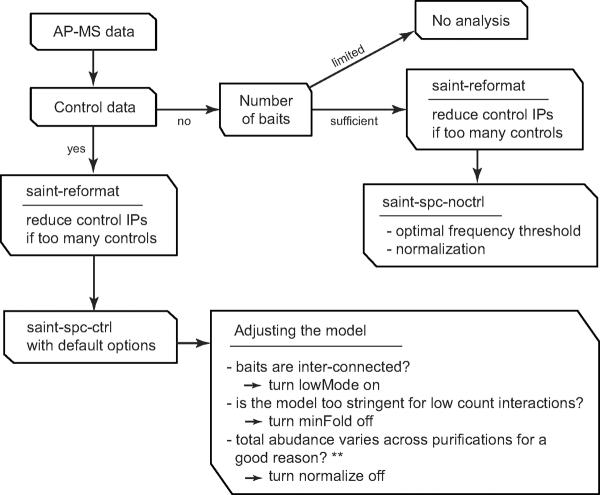
The ideal dataset for interaction scoring is one that includes a large number of baits in which each bait is analyzed in multiple biological replicates. Preferably, a sufficient number of appropriate negative control experiments should also be included: this – together with the biological replicate analysis – provides robustness in the interaction detection (see “Commentary” for a discussion of experimental design). However, such an ideal set-up is rarely possible and in practice the experimental design of AP-MS falls short in many different ways. Because of this, it is challenging to provide a `one-size-fits-all' statistical model, and adjustments should be made to the model to enable meaningful scoring of different datasets. Such adjustments are implemented in SAINT via different statistical models for spectral counts and intensity data with and without control purifications, and user-selected “options” that enable customization to the dataset at hand (Figure 1). How to use these “options” is detailed in the Basic Protocol 2.

Figure 1.

Choosing the appropriate version and optional arguments in SAINT.

BASIC PROTOCOL 1 INSTALLATION AND DATA FORMATTING

We first begin by explaining the installation of the software in the Linux environment and the steps for preparing the input files to run SAINT. The prerequisite for running SAINT is to have AP-MS data associated with quantitative information such as spectral counts, number of unique peptides, or MS1 intensity for each bait-prey interaction. Experimental design considerations are discussed in the “Commentary” section below.

Materials

Hardware

• Workstation running under Linux OS platform

Software

• GNU Scientific Library (http://www.gnu.org/software/gsl/)

• Source code for SAINT (http://saint-apms.sourceforge.net/Main.html)

• R package (http://cran.r-project.org/)

Setting up SAINT

• 1Download the source code from the SourceForge website and install by `make all' command.
• 2Move the folder to a permanent position.
• 3Download and install GNU Scientific Library for C Language.
• 4
  We also recommend adding the directory containing the executable files to the PATH variable. For instance, one can add the directory to bash shell file (.bashrc) as follows:

  • … PATH=/home/user/projects/SAINT/bin/:$PATH

Data preparation

• 5Prior to running SAINT, identify and quantify peptides and proteins from MS data using computational pipelines (Nesvizhskii, 2010).

  A typical analysis involves searching MS/MS spectra against a protein sequence database to identify peptides, statistically validating peptides to spectrum matches, mapping peptides to proteins and summarizing the data at the protein level. One commonly used data analysis tool is Trans Proteomic Pipeline (TPP; http://tools.proteomecenter.org/software.php) for processing peptide and protein identification data (Deutsch et al., 2010). With respect to the choice of the protein sequence database, for AP-MS studies we recommend using RefSeq database due to its low degree of sequence redundancy and ease of gene-level summarization of the data. Protein identifications should be filtered to eliminate most false positive protein identifications, with false discovery rate (FDR) of 1% being a commonly applied threshold.

  With respect to protein quantification, SAINT can be used with both discrete (e.g. spectral counts) and continuous (e.g. MS1 integrated peptide ion intensity) data. Spectral counts can be extracted from processed MS files using the computational tool Abacus (Fermin et al., 2011) (http://abacustpp.sourceforge.net) compatible with TPP results files. Peptide intensities can be extracted from MS data using tools such as IDEAL-Q (Tsou et al., 2010) or MaxQuant (Cox and Mann, 2008), and then used to estimate the protein abundances by summing the intensities of all peptides, or using the top 3 most intense peptide approach (Silva et al., 2006). It should also be noted that, due to presence of shared peptides, peptide level quantification is not always an unambiguous measure of protein abundance. As a result, several quantitative measures can be defined for each protein depending on whether all peptides are considered, or only unique (non-shared) peptides. For detecting non-specific binders in AP-MS data using SAINT, we recommend using all peptides, i.e. total spectral count, or total summed peptide intensity (Nesvizhskii, 2012). This represents the most conservative approach less likely to underestimate the abundance of proteins that are members of homologous protein families, many of which are common background contaminants (e.g. ribosomal proteins, tubulins, histones, etc.).

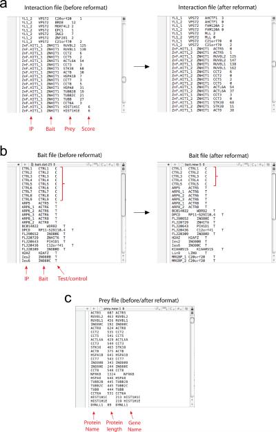
• 6Given the list of proteins identified with high confidence in the entire experiment, with associated quantitative information for each protein in individual experiments, the next step is to prepare input files for SAINT analysis. This involves preparing the prey, bait, and interaction tables in tab-delimited files, as illustrated in the SAINT vignette (included in the software release) or Figure 2.
• 7Re-open tab delimited files generated from Mac OS X or Microsoft Windows in a text editor in unix environment and re-save as unix-compatible tab delimited files. The unix utilities mac2unix and dos2unix may be used for this purpose. Alternatively, open each file in nano text editor, press Ctrl+O once for saving, and keep pressing Esc+D until the file type shows neither [DOS format] nor [MAC OS format] next to the file name. Hit the enter key to save.
• 8The interaction file should contain four columns separated by blank spaces such as tabs: purification (IP) names, bait protein names, prey protein names, and quantitative data (spectral counts, number of unique peptides or intensities). No blank spaces are allowed in the names. Associate each purification with a unique name (defined by the user), and a bait may be associated to more than one purification. SAINT will consider all purifications associated with the same bait protein name to be “replicates” and generate scores representing the likelihood of association across all replicates (see “Commentary” for bait naming conventions when analyzing biological and technical replicates, or when looking at baits analyzed under different conditions). The bait protein names and prey protein names are defined by the user (SAINT does not have requirements for these names), but it is important to ensure that there are no duplicate entries and also that the data is consistent throughout the three SAINT input files. The initial input file may not include zero observations, but preprocessing (explained below) inserts them later wherever needed. Lastly, we recommend deleting the quantitative data for the bait itself in its own purification as it is usually the highest abundance in the purification and undermines the scores of other less abundantly quantified interactors.
• 9The bait file should contain three columns: purification (IP) names and bait names (as defined in the interaction file), and target/control labels. As in the other two files, duplicate entries interfere with the preprocessing and must be avoided.

  • ### Read the bait file

    R> bait.dat = read.delim(“bait.dat”, header=F, sep=”\t”, as.is=T)

  • ### Check duplicate purification names in the bait file

    R> length(bait.dat$V1) == length(unique(bait.dat$V1))

  • ### Check duplicate bait names in the bait file

    R> length(bait.dat$V2) == length(unique(bait.dat$V2))

  • ### Check whether there is missing bait name in the bait file

    R> inter.dat$V2[!(inter.dat$V2 %in% bait.dat$V2)] ## Prints missing bait names

  Each row must provide unique information for a single purification. The pairing between purification and bait names must be consistent with the interaction file. The last column must contain one of the two letters, `T' for target data (which is all the data except for the controls) and `C' for control data. For statistical reasons, we recommend to treat each control purification as a different bait, not as replicates of single control bait. For instance, we recommend setting the bait names for control IPs in Figure 2 as “Ctrl1, Ctrl2, Ctrl3” instead of “Ctrl, Ctrl, Ctrl”. In the former case, SAINT treats all controls as repeated measures of a single control pull-down, which may result in poor mean and variance estimates for the false interaction distribution.

• 10Using the free statistical software R, quickly check whether there are duplicate names and that all names in the interaction file are in the bait file.

  • ### Read the interaction file

    R> inter.dat = read.delim(“inter.dat”, header=F, sep=”\t”, as.is=T)

  • ### Check duplicate interaction names in the interaction file

    R> inter = paste(inter.dat$V1, inter.dat$V2, inter.dat$V3, sep=” ”)

    R> length(inter) == length(unique(inter)) ## If FALSE, there are duplicate entries.

• 11The prey file for spectral count data should contain three columns: prey protein names (as defined in the interaction file), protein length, and prey gene names. The file for intensity data should contain two columns: protein names and gene names. Protein names in the first column must be unique, or redundant preys will be removed in the saint-reformat command. Typically, we use as “protein names” the identification or accession numbers as provided by the mass spectrometry search engines. These names must include all preys appearing in the interaction file, as if any protein is missing, the whole data reformatting routine stops and SAINT alerts the user to fill in the missing protein names. The second column (used for spectral count data only) is the protein length of preys (in amino acids), which can optionally be used as a normalization factor for spectral counts in the model (see command line information below). Instead of protein length in amino acids, the user can use the molecular weight of the prey protein instead, providing that the entire dataset is treated in a consistent manner. The last column should contain additional gene identification information for preys (we use the HUGO symbols for human proteins), which are usually more intuitive than protein database names, and also enable downstream mapping to gene centric databases. Note that the prey protein name and prey gene name may be identical if no cross-reference is needed and/or the protein names are intuitive.

Figure 2.

Illustration of input data in the TIP49 dataset.

Reformatting data

• 12Once the input dataset is ready, the pre-processing routine “saint-reformat” should be run first. As described in the “Commentary” section, when large numbers of control runs are available, these can be reduced into n virtual controls with the largest quantitative values. For example, to reduce the control data into 5 controls, run the command line:

  saint-reformat interaction.data prey.data bait.data 5

If no such data compression is necessary, run the same command without the last argument, i.e.:

• saint-reformat interaction.data prey.data bait.data

In either case, the command line reports three new files, interaction.new, prey.new, and bait.new. These files are the preprocessed input files for SAINT analysis. If there are inconsistencies between the input files (e.g. prey or bait names present in the interaction.new file do not appear in prey.new or bait.new files), then saint-reformat quits preprocessing and advises the user to rerun after filling in the missing items in those files.

Basic Protocol 2

Running SAINT

Once the data has been prepared and reformatted as described in the Basic Protocol 1, SAINT proper can be run. As discussed in the introduction and the Commentary, SAINT utilizes different statistical models for different types of quantitative data and experimental designs which are accessed by different arguments in the command lines. The meaning of the different SAINT options is reviewed in this section.

Materials

• Installed SAINT software and reformatted input data

• R package (http://cran.r-project.org/)

As explained earlier, different versions and options are available depending on the data type and experimental design.

• For spectral count data with control purifications, SAINT uses the three input files and five additional arguments specifying the type of statistical model to be used. The command line for running SAINT in this mode is:

  • saint-spc-ctrl interaction.new prey.new bait.new 2000 10000 0 1 1
    (different arguments, or “options”, are defined below; the default values are listed here)
• 2
  If the user wishes to provide a seed for the random number generator, this should be specified before the command line, as follows:

  • GSL_RNG_SEED=123 saint-spc-ctrl interaction.new prey.new bait.new 2000 10000 0 1 0

  where the example seed 123 can be any integer number. Including the random seed ensures identical scoring results for the same dataset analyzed at different times or on different computers. If the seed is omitted, SAINT scores may change by a few decimal points on different runs of the same dataset.

  Options:

  1. The argument 2,000 is the number of sampling iterations for the burn-in period of Markov chain Monte Carlo (MCMC). We found this number to be sufficient in most instances, though higher values can be used for more robust inference.

  2. The argument 10,000 indicates the number of sampling iterations in MCMC for actual inference. Once again, while we have found this number to be appropriate, higher values can be used.

  3. The lowMode option (0 off – default; 1 on) indicates whether SAINT should take into account the presence of weak and strong interactions for each prey, so that it does not penalize the weaker interactions as severely. In the default (off) set-up, low count interactions tend to be penalized if the same prey has an extremely high count interaction with one or more other bait(s). When the dataset consists of only a few baits or densely interconnected baits, we recommend turning this option on (alternatively, the user can explore the option of analyzing each bait separately against the control data). When turned on, the “lowMode” option applies by default to preys with interactions in 100 counts or more. This default value can be increased or decreased in the source code (_LM_ in the header file).

  4. The minFold option (0 off; 1 on - default) determines whether to enforce a minimum fold separation rule between true and false interaction distributions. When turned on, the model assumes that the mean value of the true interaction distribution is at least ten fold higher than that of the false interaction distribution, where the latter is estimated from the control purifications. While turning on this option is more stringent, there are cases (particularly when some of the true interactors are also common contaminants) where turning off this option is useful. We recommend turning off this option only if the overall quality of the dataset is high, and in particular, if the purifications of the baits and controls are truly matched. The ten fold requirement can be adjusted in the source code, by changing _fold_ variable at the top of the header file in SAINTspc-ctrl folder (v2.3.3 or later uses five fold by default).

  5. The normalize option (0 off; 1 on - default) determines whether to divide spectral counts by the total spectral counts in each purification. Like minFold, turning on this option is usually more conservative for scoring, as the control runs typically have less identifications than the bait runs; again, turning off this option should only be performed with data of high quality. Note, however, that the normalization option may artificially boost scores associated with baits in which not much interactions are detected, especially in the datasets where many of the other baits interact with one another and share many common preys. We therefore recommend to always have a visual inspection of the results to identify problematic cases.

• 3
  For intensity data analysis with controls, the general preparation of the input files (inter.dat, bait.dat, prey.dat) is identical as described above for the spectral count model with controls, with one exception: the protein length is not required as it will not be utilized for normalization. Also note that the options “lowMode”, “minFold” and “normalize” options were developed to accommodate the Poisson model of count-based data. The probability model from intensity data is much more adaptive (Gaussian model) and seems to work well without these additional parameters. The command line(s) with and without seed for the random number generator are:

  • saint-int-ctrl interaction.new prey.new bait.new 2000 10000
  • GSL_RNG_SEED=123 saint-int-ctrl interaction.new prey.new bait.new 2000 10000

  where the two numbers at the end of the command line are the number of sampling in the burn-in and main iterations.
• 4For spectral count data without control data, the files are prepared in the same manner (with the exception that the bait file lacks the column C / T). However, SAINT incorporates different arguments, which are defined in the command line(s) as:

  • saint-spc-noctrl interaction.new prey.new bait.new 2000 10000 0.2 0.1 0 1

  • GSL_RNG_SEED=123 saint-spc-noctrl interaction.new prey.new bait.new 2000 10000 0.2 0.1 0 1

  Options:

  1. The argument 0.2 (first option term after the number of sampling iterations) specifies the frequency threshold `fthres'. All preys with non-zero spectral counts in greater than (100×fthres)% of the purifications will be considered as zero probability interactions. Thus the example command above will remove all interactions for preys appearing in 20% of the purifications.

  2. The next argument `fzero' determines the proportion of zero spectral count data to be included in the estimation of the false interaction distribution. To explain this, let us call N the total number of purifications. For instance, consider 0.1 (or 10%) and set T = N × 0.1, i.e. 10% of the total number of purifications. This option tells the software that, if a prey has M non-zero spectral counts (M < T), then use (T–M) zero data for estimation. Using additional zero data helps the model learn the fact that preys appearing in fewer baits are likely specific interactors, not frequent flyers. In rare circumstances, the user may want to consider all non-detection as zero data, particularly in smaller datasets with no controls (.e.g 10 baits or less), `fzero' can be specified as any number greater than the `fthres' parameter above. In most applications, we recommend users to set this value so that (fzero×N) ~ 5 in general.

  3. The variance modeling option (0 off - default; 1 on) must be specified to determine whether the variance parameter should be included in the model. This argument tells the software whether to use a generalized Poisson distribution with a dispersion parameter, instead of a plain Poisson distribution with mean parameter only. The recommended value is 0 unless there are at least three replicate purifications for all baits.

  4. The normalize option (0 off; 1 on) determines whether to divide spectral counts observed for a prey by the total spectral counts for all preys detected in a purification. If there is a significant variation in the number of possible interactors across baits, the recommended value is 0. Otherwise, the recommended value is 1.

Sorting interactions

All the routines explained above generate multiple output files in various formats. The main output file is reported in the “unique_interactions” file in the RESULT folder. This file has the list of all unique bait-prey pairs with the corresponding probability scores in the column called “AvgP”; AvgP is simply the average of all individual SAINT probabilities (iProb) for a given prey across all replicates of a given bait. The file also contains a column called “MaxP”, which reports the largest probability (iProb) of a bait-prey pair across all replicate purifications.

• 5To select high confidence interactions, open the unique_interactions file in a spreadsheet using software such as Microsoft Excel, and sort the data in a decreasing order of AvgP.
• 6Choose a desired threshold and select all interactions passing the threshold (typically a SAINT probability threshold between 0.7 and 0.9, or even higher depending on the desired stringency of filtering). The selection of the threshold can be assisted by plotting a ROC-like curve (e.g. a curve that plots the number of protein interactions passing the filter that are known interactions vs. the total number of interactions passing the filter, for a range of probability filters) based on protein interaction data annotated in the existing protein interaction databases (or in compendiums of interactions such as iRefWeb (Turner et al., 2010) or PSICQUIC (Aranda et al., 2011)).
• 7To analyze the probability scores for each replicate, open “interactions” file, which expands the unique_interactions file by listing every purification-prey pairs instead of bait-prey pairs. In this file, the user can look at iProb column for the probability score in the individual replicates.
• 8
  In the same folder, SAINT reports a matrix-formatted output file as well, where the preys and the purifications/baits are listed in the rows and columns of the data matrix respectively, along with their raw quantitative data and the probability scores (matrix_form file). To select all interactions with the posterior probability greater than or equal to 0.8:

  • R-CODE: selecting high-confidence interactions
    ### read data and remove self-self interaction
    d = read.delim(“unique_interactions”, header=T, as.is=T)
    d = d[d$Prey != d$Bait,]
  • ### run the following three lines if interested in bait-to-bait interaction only
    bait = unique(d$Bait)
    id = d$Prey %in% bait.
    d = d[id,]
  • ### select high confidence interactions (0.8 and above)
    d = d[d$AvgP >= 0.8,]
  • ### write out the resulting table to a file
    write.table(d, “filtered_interactions”, sep=“\t”, quote=F, row.names=F)

Support Protocol 1: Visualization of network

This script generates the final report for table view as well as network visualization in Cytoscape (Shannon et al., 2003). Here we describe how to generate the input file for Cytoscape and how to utilize the quantitative data to improve visualization.

Materials

Software

• Cytoscape (http://www.cytoscape.org/)

• R package (http://cran.r-project.org/)

1. If needed, create a node attribute file by listing a unique list of proteins combining baits and preys, and format each row as follows:

   • R-CODE: creating node attribute file
   • d = read.delim(“filtered_interactions”, header=T, as.is=T)
   • prot = unique(c(d$Bait, d$Prey))
   • nprot = length(prot)
   • type = rep(“prey”, nprot)
   • type[prot %in% d$Bait] = “bait”
   • nodeAttr = data.frame(Protein=prot, Type=type)
   • write.table(nodeAttr, “nodeAttr.txt”, sep=“\t”, quote=F, row.names=F, col.names=F)

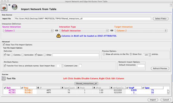
2. Open Cytoscape and import network data from the “filtered_interactions” file by selecting “Network from Table” under File menu (Figure 3). Select file name, set source and target interactions to bait (Column1) and prey (Column2) columns, respectively. Click on “Show Text File Import Options” in the “Advanced” box to ensure that the delimiter is set to Tab. In the preview box, click on the unselected columns to import them as edge attributes. Click Import button at the bottom.

3. Import prey attribute data from a text file by “Attribute from Table (Text/MS Excel)” under the FILE menu.

4. (OPTIONAL) Click on the VizMapper tab on the left and choose “Nested Network” as the visualization style.

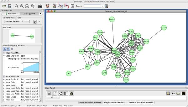
5. In the pull-down menu, choose “Layout” → “Cytoscape Layouts” → “Edge-Weighted Spring Embedded” → “Spec”. This operation reorganize nodes based on the degree of connectivity between proteins additionally weighted by the quantitative strength of each interaction (Figure 4).

6. (OPTIONAL) Different node sizes and colors can be selected for the baits and preys using the prey attribute information in the Visual Mapping Browser tab. Additionally, the edge thickness may be mapped to indicate the quantitative information for each bait-prey interaction.

7. Make adjustments to optimize the visibility of nodes to complete visualization of the network. Export the graph into pdf file if needed (“File” → “Current Network View as Graphics”). Note that the resulting pdf file can be further refined in graphic software such as Adobe Illustrator.

Figure 3.

Importing the SAINT result files into Cytoscape for the analysis of the TIP49 dataset.

Figure 4.

The network visualization of the TIP49 dataset in Cytoscape.

Alternate Protocol 1: Running SAINT through ProHits interface: virtual machine GUI

SAINT may also be run without the unix / command line interface, using the ProHits graphical user interface (Liu et al., 2010). In this case, the search results (Mascot, X!Tandem, SEQUEST or other search engines via the Trans Proteomic Pipeline) can be uploaded directly to ProHits and all tables for SAINT can be generated, and options selected, through ProHits. Alternatively, SAINT can be run on pre-generated bait.dat, prey.dat and inter.dat files (this enables the user to avoid using the command line-based Linux system). ProHits/SAINT may be run on a Mac OS X or PC Windows using a virtual machine package available at ProHitsMS.com (installation instructions, user manuals and instructional videos are also available at ProHitsMS.com; also see accompanying protocol by Liu et al., 2010).

To run SAINT from the ProHits VM, download and install the software package on your computer, and set-up projects and user privileges (as described in Liu et al., 2010). The key steps to enter your data in ProHits and analyzing it with SAINT are described here. Steps A-E are used for running SAINT from mass spectrometry search results; if using predefined SAINT-compatible files, skip to the end of section C.

Materials

Hardware

• A computer running OS X (we tested 10.6.8) or Windows (XP or 7) with at least 50 GB free disk space.

Software

• Virtual machine software (VirtualBox for Mac OS X from https://www.virtualbox.org/ or VMware Player for Windows PC from http://www.vmware.com/products/player/overview.html)

• ProHits Lite VM VirtualBox version (CentOS57_ProHits_VirtualBox for Mac OS X or CentOS57_ProHits_win for Windows PC) from http://prohitsms.com/

• Mass spectrometry search results, generated by Mascot (*.dat), X!Tandem (*.xml), SEQUEST (*.tar.gz) or the Trans-Proteomic Pipeline (PeptideProphet and ProteinProphet *.xml files are both required).

1. Create baits, experiments and samples within a “Project” (the “Project” should be predefined)

   ProHits is organized in a hierarchical fashion. A “bait” (e.g. tagged protein) can be associated with several experiments (e.g. different biological replicates or growth conditions), and each “experiment” can be associated with several samples (e.g. technical replicates, or different fractions from the same experiment). The essential point is that the user will need to create as many “samples” as MS/MS database search results files (each file needs to be associated to a single “sample”). ProHits can handle search results from gel-based workflows in a dedicated module (e.g. if tracking by molecular weight is desired), or search results from any kind of workflow in the “gel-free” sample creation.

   Create a new sample by selecting “Create New Entry”, and select “Add Gel-free sample” on the left menu of the ProHits Analyst (within the selected project). Follow the navigation steps to create and annotate the desired baits, experiments and samples. It is highly recommended to utilize ProHits as an electronic notebook, and provide detailed annotation of the experiments.

2. Transfer .MS/MS search results to each sample

   ProHits has an upload function which enables import of search results generated by the search engines Mascot (Perkins et al., 1999) (*.dat), X!Tandem (Craig and Beavis, 2004) (*.xml) and SEQUEST (Yates et al., 1995) (*.tar.gz). Results from these and other search engines may also be imported after running the data through the TPP pipeline. In this case, both pep.xml and prot.xml (the output from TPP's PeptideProphet and ProteinProphet tools) files need to be uploaded.

   Under the “Create New Entry” menu item, select “Upload Search Results”, and click on the upload icon in the Options column next to the desired sample. Select the type of result file to be uploaded and browse the computer hard drive to retrieve the file. Click “Submit” to complete the upload.

3. Run SAINT

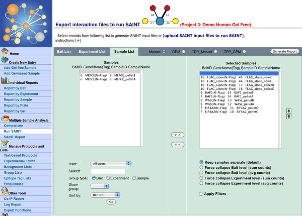
   Once the desired number of samples and negative controls is uploaded, select “Run SAINT” under the “Multiple Sample Analysis” section of the left menu bar. This opens a new page where the data can be viewed at the level of baits, experiments or samples (see Figure 5). Select the desired files from the left box and use the arrow buttons to transfer to the right box. By default, SAINT considers each sample separately even when using the bait or experiment level view. To force collapsing at the level of the bait or experiment (e.g. when looking at technical replicates or different fractions from the same bait), select the desired option under the right hand box. Note that - while ProHits enables the user to prefilter the files (e.g. to remove common contaminants) prior to running SAINT - this is not recommended for most applications (filtering to remove low quality protein identifications, e.g. those above 1% FDR, is however recommended).

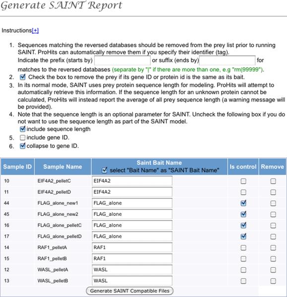
   Once all the desired files have been selected, the button “Generate Report” is used to bring up a new navigation window in which the control runs can be specified, the names of the files modified (SAINT will automatically group files with the same bait name), and desired options selected (see Figure 6). After this is done, the button “Generate SAINT Compatible Files” instructs ProHits to retrieve the prey length from its internal protein database, and generate the three files required to run SAINT (prey.dat, bait.dat and inter.dat). ProHits will provide the option to download the files on the user's hard drive, or to run SAINT directly within ProHits.

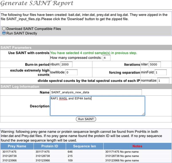
   Selecting “Run SAINT Directly” will open a new panel enabling to select the SAINT parameters (as defined above, Figure 7). If using ProHits to run SAINT from previously generated files, this navigation panel enables to upload the files and select the parameters. “Run SAINT” instructs ProHits to begin the analysis.

4. Explore SAINT results

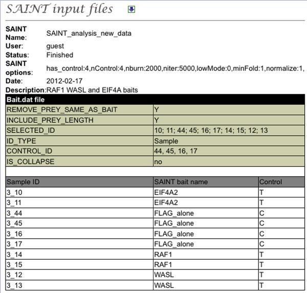
   SAINT results can be explored via the “SAINT Report” link from the “Multiple Sample Analysis” left hand menu. This will bring up a list of all SAINT analyses performed in this project. In the option column, the download icon enables the user to directly download the SAINT report folder. The “page” icon lists all the samples, controls and options used for SAINT analysis to facilitate tracking and ensure transparent reporting (Figure 8). Note that SAINT can be re-run on the same files using different options by selecting the “rerun” icon.

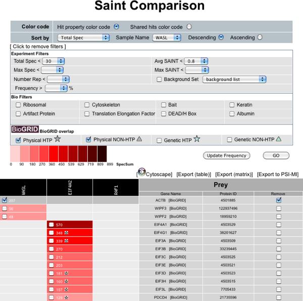
   Lastly, the SAINT results can be visualized, and further analyzed using the “graph” icon. This opens up a new window, called “SAINT comparison”, which displays the results as a table, with baits in columns and hits in rows. By default, the table displays the maximal SAINT score for each prey across all baits, and is unfiltered. To filter the results, select “Click to apply filters” towards the top of the page. Select the desired SAINT score (either average SAINT - AvgP - or maximal SAINT value - MaxP), and other filters, as desired. Click on the “Go” button to apply the desired filter sets (Figure 9). It is also possible to manually remove entries from the final report by clicking the check boxes located in the table and pressing “Go”. The selected entries will be greyed out (note that a list of manually removed entries is provided in the exported Excel files for transparent reporting of the data). Lastly, it is possible to check which interactions have previously been deposited in the BioGRID interaction (Stark et al., 2011) database by clicking on the selected types of interactions in the “BioGRID overlap” panel and pressing “Go”. Interactions reported in BioGRID will be marked by stars or triangles in each cell.

5. Report SAINT results

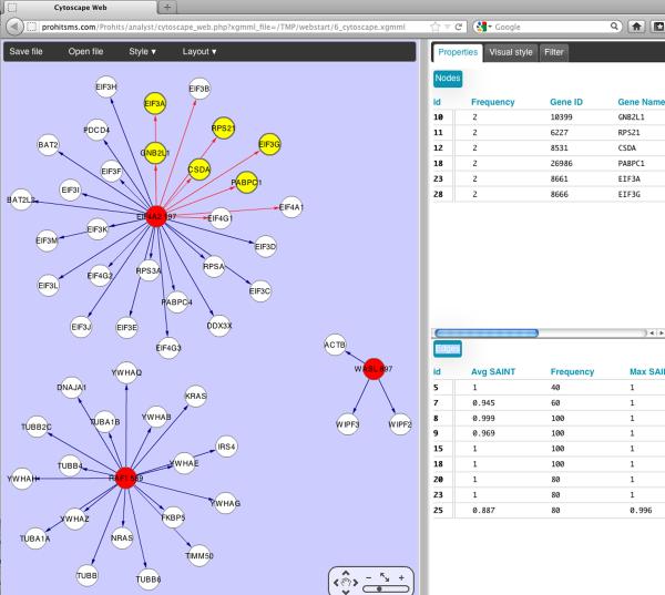
   ProHits facilitates the visualization of the SAINT filtered results by enabling direct graphical visualization in Cytoscape Web (Lopes et al., 2010) (Figure 10). Filtered data can also be downloaded either in a “table” format (very similar to the unique_interaction file generated by SAINT as described above), or as a matrix format (which is essentially the same view as displayed in the ProHits SAINT Comparison page). In either case, the filters applied and the manually removed interactions will be listed at the top of the report, to facilitate reporting. Lastly, the data analyzed by SAINT can also be prepared for submission to interaction databases by selecting the “Export to PSI-MI” button. This will open a new navigation window where you will be prompted to fill in the information to prepare the PSI-compatible files.

Figure 5.

Select samples to analyze using the ProHits interface.

Figure 6.

Define controls and samples and select parameters for file preparation.

Figure 7.

Select SAINT options and initiate analysis within ProHits.

Figure 8.

Tracking of the SAINT analysis parameters in ProHits.

Figure 9.

Graphical user interface to explore SAINT results.

Figure 10.

Automated Cytoscape generation of SAINT results from ProHits.

GUIDELINES FOR UNDERSTANDING RESULTS

Analysis of TIP49 dataset

Using the command line version of the software, we illustrate a SAINT analysis of the TIP49 dataset for an example of spectral count data with control purifications. This human PPI dataset was generated for key protein complexes involved in chromatin remodeling (Sardiu et al., 2008), namely Prefoldin, hINO80, SRCAP, and TRRAP/TIP60 complexes. The dataset consists of 27 baits (35 purifications) and 1207 preys with 5521 unfiltered interactions.

1. Compressing control samples with different number of replicates

While 35 negative control purifications were included in the dataset, we reduced the control purification data into 9 virtual negative controls, each taking the largest spectral counts from respective replicate purifications for each prey (at this step, we performed this control reduction without using the saint-reformat option).

2. Reformatting the input files

We next performed data preprocessing (saint-reformat) on the TIP49 dataset. Figure 2 shows the interaction, bait, and prey data before and after this step. In saint-reformat, we specified K=5 to get the 5 largest spectral counts from the controls, resulting in further data reduction (for more stringent filtering; can be waived by K=9). A notable change in the interaction file is that interactions are reordered by pairing replicate observations for the same bait-prey pair, and more importantly, that zero counts are inserted in the data (Figure 2a). For the bait file, note that the control purifications were reduced to a smaller set as specified, by taking the largest five spectral counts in control purifications for each prey (Figure 2b). The prey file was not modified since it changes only if there are duplicate entries in the file.

3. Running SAINT

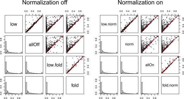
Following saint-reformat, we ran SAINT with 2,000 burn-ins and 10,000 main iterations. We did consider all combinations of lowMode, minFold, and normalize options. Figure 11 shows the comparison of the probability estimates between every combination of options, where the biggest difference is made when minFold options is turned on and off.

Figure 11.

Comparison of probabilities using different options in the TIP49 dataset.

4. Visualization

Taking the results from the analysis with lowMode=off, minFold=on, and normalize=on, we used the R scripts in the previous section to generate Cytoscape input files for network visualization.

COMMENTARY

Background Information

Here, we will review key features in the experimental design that influence the selection of model parameters such as control purification and replicate analyses, and address issues related to specific types of datasets. The following considerations apply to both count and intensity data, but for simplicity, we will use spectral count-based scoring as an example.

Control purifications

In terms of scoring, control data provide direct quantitative evidence for non-specific binders. Therefore, an interaction can be regarded as statistically significant if the quantitative evidence for the interaction is stronger than that in the control purifications. Recently, examples of datasets incorporating such control data have been generated, e.g., for chromatin remodeling complexes, such as the TIP49 data that we used above (Sardiu et al., 2008) and the human protein phosphatase PP2A system (Glatter et al., 2009; Goudreault et al., 2009). These datasets include several to tens of control purifications representing a robust background of non-specific interactions, which allow the statistical model to identify representative quantitative distributions for non-specific (false) and specific (true) interactions in purifications of real baits. Each putative interaction is referenced against the two (true and false) distributions, and the probability that the interaction is from the true interaction distribution is reported as the score.

For meaningful scoring, experiments should be designed with a sufficiently large number of `relevant' control purifications to identify as many non-specific binders as possible. In control data, however, some non-specific binders are captured inconsistently across different control purifications. Given these two facets of control data, the optimal strategy can be phrased as (i) design controls that appropriately represent the source of non-specific binders in the purification of real baits, (ii) generate a sufficiently large number of control samples to learn the consistency of non-specific binding, (iii) select for analysis those control purifications showing the highest degree of consistency in the detection of contaminants. Another point to consider in the design and implementation of negative controls is that each batch of purifications (defined here as purifications performed at the same time, and/or using the same set of reagents) may retrieve a different subset of non-specific interactors. It is therefore important to perform negative controls in parallel to bait purifications. How many controls are optimal for SAINT analysis? For SAINT modeling to be accurate, three to five appropriate control purifications are minimally required. Perhaps counter intuitively, however, a very large number of control runs do not necessarily offer a perfect solution. For example, if a prey is detected in a small proportion of controls (meaning that in some controls it will have a quantitative value of 0), the false interaction distribution will be underestimated, mistakenly allowing such contaminants to be scored as specific binders. To address this, SAINT provides a routine to select a fraction of consistent control data with the function “saint-reformat” (detailed in the protocol above). Using this function, the user can extract the K largest spectral counts / intensities from the control data for each prey when the data have more than K controls (default K=5, arbitrarily chosen based on experience).

Replicate analyses

Another important aspect of the experimental design is the number of biological replicate purifications for baits. Replicate purifications can improve the robustness of scoring for an obvious reason: they allow the assessment of the reproducibility of high confidence interactions, which cannot be evaluated in experiments with a single purification per bait. In addition, the best replicate design is a perfectly balanced design in which every bait is analyzed with the same number of replicates. Regardless of the scoring metric chosen, the imbalance in the number of replicates creates a bias for or against the baits with more replicates, depending on how the evidence is summarized from replicates. For instance, SAINT scores (AvgP) tend to be more generous for the interactions with fewer replicates, which is intuitive since more replicate purifications will reveal irreproducible preys that are usually assigned low probability scores. On the other hand, the specificity of scores will be higher for the baits associated with more replicates. SAINT computes, in addition to the standard SAINT scores (AvgP), individual probability (iProb) values for each sample, as well as the MaxP value (the largest iProb). In some challenging datasets for which multiple biological replicates were available, we have found that taking the best n iProb (e.g. best 2 of 3; best 3 of 4) enabled more sensitivity for the detection of the less reproducible interactions (for example, interactions with are condition-dependent). We are suggesting to always thoroughly inspect the dataset, and to select the most appropriate scoring method.

There are two broadly defined types of replicates in AP-MS experiments: technical replicates and biological replicates. Here, we use the term “technical replicate” to indicate the case where a single purification is performed on a biological sample and MS analysis is performed multiple times. By contrast, we use “biological replicate” for the case where generation of the biological material, purification and MS analysis are done independently. In our experience, the lack of reproducibility in AP-MS data is more often associated with the preparation of biological material (e.g. cell growth and lysis) and purification (e.g. immunopurification, elution, tryptic digest) than from the LC-MS/MS analysis. For this reason, we recommend that the reproducibility of interactions should be monitored at the level of biological replicates. For biological replicates, the most stringent approach is to make sure that these are as different from each other as would real baits and controls be (using a standardized protocol). For instance, cells can be grown/harvested on different days, purifications performed in different batches, mass spectrometry done separately, using a randomized order for the loading of the samples (see Figure 12). The latter is important for minimizing the possible carry-over issues in LC-MS/MS (i.e. detection, in the current sample, of proteins from the preceding sample when both samples were analyzed using the same LC column).

Figure 12.

Ideal design of an AP-MS experiment with negative controls and biological replicates. Hypothetical experiment involving the purification of four different baits (colored circles) and a negative control (grey circle). Each of the biological replicate experiments is performed for each of the baits in a single batch. Different biological replicates are performed on batches of cells harvested at different times, and for which purification and proteolysis is done on different days. Notice the randomization of the loading order of the samples on the mass spectrometer to help preventing bias (e.g. carry-over).

If technical replicate data is available, we suggest that these should be merged into a single virtual sample before running SAINT. If all baits have the same number of technical replicates, one can simply sum spectral counts or intensities. This results in increased quantification values overall, which is especially useful for obtaining a higher SAINT score from low spectral counts. If some baits have more technical replicates than others, we recommend averaging spectral counts or intensities across all baits, treating missing data as zero values, and rounding up the average to the nearest integer (rounding “up” prevents data loss). In the case of fractionated samples (for example by SDS-PAGE), it is recommended that each of the fractions (by opposition to only selected fractions, e.g. gel bands) be run in the mass spectrometer to prevent bias and that the results of all fractions be summed up prior to SAINT analysis.

Another important question is how many biological replicates should be generated for each bait. Even though it is desirable to generate multiple replicates for each bait, time and cost considerations often limit this in real life scenarios, especially in large-scale studies. Our own studies now include two or three true biological replicates per bait analyzed. A last note regarding the biological replicates: before using SAINT, the quality of replicates should be manually examined (e.g. using ProHits software (Liu et al., 2010), or a pairwise scatter plot of spectral counts or intensities between biological replicates). In the SAINT analysis, including a clearly defective sample (lower bait or prey abundance, or detection of high amounts of contaminant proteins) has negative effects, including “dilution” of the signal and loss of bona fide interactions. If such a case is detected, we suggest that the defective purification be replaced by a new biological replicate. This also applies to negative control runs; in particular, negative controls in which the previous bait analyzed is detected in significant amounts due to carry-over issues should be avoided to involve penalizing true interactors in the remainder of the dataset.

Note that if the goal of an experiment is not just to find interaction partners for a specific bait, but rather to identify differentially-regulated interactors (e.g. after the cells expressing the bait have been subjected to some treatment), the samples purified under different conditions should not be considered as biological replicates, but as completely different experiments. Another special case is when different purifications of the same bait are performed using multiple epitope tagging strategies or affinity purification conditions. In this case, we recommend running separate analysis for each type of purification (using matched controls in each case) and taking the union or the intersection for the selected interactions, as appropriate.

Small or interconnected datasets: implementation of new “options”

In contrast to the ideal cases described above where multiple baits are analyzed using the same experimental conditions, real datasets are often generated for a small collection of baits, and even for a single bait. SAINT is still applicable to this kind of datasets. We recently demonstrated that SAINT can distinguish true interactions in the case of human phosphatase PP5 and the “frequent-flier” chaperone HSP90 (Skarra et al., 2011), showing that it is able to identify true interactions even for the proteins frequently identified in controls if quantitative data is stronger in real bait purifications. While appropriate negative control experiments and sufficient replicate purifications are always important for scoring any dataset, these are absolutely critical for careful scoring of “frequent-fliers” in smaller datasets.

While SAINT (with proper controls and replicates) performs well for one bait, or a small number of baits which do not share many interaction partners, we also observed that the previously published version (v2.2.3 or earlier) was underscoring some true interactions for preys associating with two or more baits in the dataset in very different abundances: in such cases, only the interactions with stronger quantitative data were assigned high probability. This occurred frequently when the baits were “interconnected”, which happens when the dataset is generated for a specific biological function, or even a protein complex. This underscoring happens because the statistical model built in SAINT has a `black-and-white' classification scheme, ignoring the possibility of weak and strong bona fide interactions. Thus SAINT identifies weak interactions as non-specific identifications and only considers the strong interactions as bona fide interactions. This can be addressed by running SAINT analysis for each bait separately for this type of datasets (or running SAINT separately on subsets of baits, when such subsets can be clearly defined). As discussed in the protocol section, we also implemented a new option `lowMode' so that the distribution representing true interactions more accurately captures lower abundance interactions. In datasets consisting of baits that are interconnected but have very different characteristics, e.g. different number of interactors per bait, both strategies (lowMode option or separate SAINT analysis) may need to be explored.

Although we previously employed SAINT successfully in small datasets, such as the one surrounding PP5 and HSP90, the standard SAINT scoring also has features that are not optimal for datasets with few baits, e.g. single bait datasets. When each prey has interactions with only a few baits, SAINT has insufficient data to estimate the true and false interaction distributions robustly. In this case, SAINT not only borrows statistical information from the population of proteins (all other proteins in the data), but also activates an explicit rule that the mean of the true interaction distribution be 10 times greater than the mean of the false interaction distribution (note that this is not the same as looking at the ratio of observed counts between real purifications and controls). This measure was an empirically optimized feature in the original version of SAINT (for spectral count data only), which effectively removed many spurious interactions on the low spectral count range that were assigned high probability just because control data had many zero counts. However, this threshold rule can also remove real interactions with large spectral counts in small datasets, which is why we included here another new option, `minFold', that can enable the user to turn off this feature when analyzing small datasets.

Lastly, we discovered that the normalization of quantitative measures, especially the practice of dividing spectral counts and intensities by the total sum within each purification, can affect the results significantly, especially when control purifications yield smaller total abundance compared to the purification of real baits. Such a normalization procedure inflates quantitative values in the controls relative to more abundant purifications of real baits, and therefore winds up decreasing the real signal. The same is true for the baits with fewer interactors, for which on average the scores will be boosted. To enable a more flexible scoring, we therefore also included a third new option called `normalize' so the users can choose whether or not to use normalization based on total spectral counts (this feature has not been implemented for intensity data yet).

When control purifications are not available

In the absence of control purifications, whether each protein is binding specifically or not to a bait is best indicated by how often the protein co-purifies across all purifications, i.e. frequency-based specificity. The frequency information was successfully utilized to filter the data in combination with quantitative data and reproducibility information in recent studies (Breitkreutz et al., 2010; Sowa et al., 2009). In these datasets, it was expected that bona fide interactions of a prey occur with a specific subset of baits, whereas non-specific binders are generally captured in random sets of purifications with high frequency. However, an obvious limitation to the experimental design lacking controls is that the frequency can be accurately estimated only when there are many baits (typically >20) and filtering based on frequency only works well when the target network is sparse. This limitation applies to all scoring methods that do not take controls into account, including CompPASS and SAINT (without controls) (Behrends et al., 2010; Breitkreutz et al., 2010; Choi et al., 2011; Sowa et al., 2009). Moreover, it is difficult to estimate true and false interaction distributions for many preys that appear with just a few baits, since there is no direct information equivalent to control data to represent non-specific binding. Hence in practice it is important to guide the model with user-specified parameters such as the optimal frequency cutoff for removing frequently appearing contaminants and the reproducibility of interactions over replicates.

Reporting SAINT results

With the implementation of these different options in SAINT, it is important to provide information about the selected parameters when reporting SAINT analysis results. This is necessary since the same scoring results need to be reproduced if one wishes to reanalyze published datasets. When reporting the results, we recommend that the user provide the following information. First, because the scores depend of the exact dataset composition, a list of all baits and control samples included in the analysis must be provided. The details concerning the search engine parameters and database used for searching should be provided as in every mass spectrometry experiment (Taylor et al., 2007). It should also be described how spectral counts were computed (e.g. using all or unique peptides only, see below). Second, the SAINT software version should be specified (e.g. SAINT-v.2.3.1): a future user should be able to track all the changes made since the specified version from the software development log file. Third, the user should report all modeling options including:

• (i)lowMode/minFold/normalize options in the spectral count data analysis with controls
• (ii)frequency and normalize options in the spectral count data analysis without controls

Last, but not least, is the description for the handling of control data, especially if there was any compression of controls over technical replicates before data formatting routine, or whether controls were reprocessed during the data formatting routine (saint-reformat).

Transparency in reporting the data is critical (Orchard et al., 2007). In addition to the selected cut-off for SAINT, a user may want to apply additional filtering, e.g. based on a minimum number of unique or total peptides detected for a prey; the exact parameters used for filtering should be reported in the manuscript. Lastly, if manual exclusion is performed, the list of the proteins removed manually should also be provided.

In this protocol, we described the critical steps for data preparation and key features that influence the statistical model and the final confidence score in SAINT. After all, SAINT computes the confidence scores solely based on quantitative data and does not explicitly incorporate relevant biological or biochemical information, and therefore it is crucial to have the data generated from appropriate experimental design to allow unbiased, reproducible, and statistically powerful scoring.

Literature Cited

- Aranda B, et al. PSICQUIC and PSISCORE: accessing and scoring molecular interactions. Nature methods. 2011;8:528–9. doi: 10.1038/nmeth.1637. [DOI] [PMC free article] [PubMed] [Google Scholar]
- Behrends C, Sowa ME, Gygi SP, Harper JW. Network organization of the human autophagy system. Nature. 2010;466:68–76. doi: 10.1038/nature09204. [DOI] [PMC free article] [PubMed] [Google Scholar]
- Breitkreutz A, et al. A global protein kinase and phosphatase interaction network in yeast. Science. 2010;328:1043–6. doi: 10.1126/science.1176495. [DOI] [PMC free article] [PubMed] [Google Scholar]
- Choi H, Glatter T, Gstaiger M, Nesvizhskii AI. SAINT-MS1: Protein-Protein Interaction Scoring Using Label-free Intensity Data in Affinity Purification-Mass Spectrometry Experiments. Journal of proteome research. 2012;11:2619–24. doi: 10.1021/pr201185r. [DOI] [PMC free article] [PubMed] [Google Scholar]
- Choi H, et al. SAINT: probabilistic scoring of affinity purification-mass spectrometry data. Nature methods. 2011;8:70–3. doi: 10.1038/nmeth.1541. [DOI] [PMC free article] [PubMed] [Google Scholar]
- Cox J, Mann M. MaxQuant enables high peptide identification rates, individualized p.p.b.-range mass accuracies and proteome-wide protein quantification. Nature Biotechnology. 2008;26:1367–1372. doi: 10.1038/nbt.1511. [DOI] [PubMed] [Google Scholar]
- Craig R, Beavis RC. TANDEM: matching proteins with tandem mass spectra. Bioinformatics. 2004;20:1466–7. doi: 10.1093/bioinformatics/bth092. [DOI] [PubMed] [Google Scholar]
- Deutsch EW, et al. A guided tour of the Trans-Proteomic Pipeline. Proteomics. 2010;10:1150–1159. doi: 10.1002/pmic.200900375. [DOI] [PMC free article] [PubMed] [Google Scholar]
- Fermin D, Basrur V, Yocum AK, Nesvizhskii AI. Abacus: a computational tool for extracting and pre-processing spectral count data for label-free quantitative proteomic analysis. Proteomics. 2011;11:1340–5. doi: 10.1002/pmic.201000650. [DOI] [PMC free article] [PubMed] [Google Scholar]
- Gingras AC, Gstaiger M, Raught B, Aebersold R. Analysis of protein complexes using mass spectrometry. Nature reviews. Molecular cell biology. 2007;8:645–54. doi: 10.1038/nrm2208. [DOI] [PubMed] [Google Scholar]
- Glatter T, Wepf A, Aebersold R, Gstaiger M. An integrated workflow for charting the human interaction proteome: insights into the PP2A system. Mol Syst Biol. 2009;5:237. doi: 10.1038/msb.2008.75. [DOI] [PMC free article] [PubMed] [Google Scholar]
- Goudreault M, et al. A PP2A phosphatase high density interaction network identifies a novel striatin-interacting phosphatase and kinase complex linked to the cerebral cavernous malformation 3 (CCM3) protein. Mol Cell Proteomics. 2009;8:157–71. doi: 10.1074/mcp.M800266-MCP200. [DOI] [PMC free article] [PubMed] [Google Scholar]
- Liu G, et al. ProHits: integrated software for mass spectrometry-based interaction proteomics. Nature biotechnology. 2010;28:1015–7. doi: 10.1038/nbt1010-1015. [DOI] [PMC free article] [PubMed] [Google Scholar]
- Lopes CT, et al. Cytoscape Web: an interactive web-based network browser. Bioinformatics. 2010;26:2347–8. doi: 10.1093/bioinformatics/btq430. [DOI] [PMC free article] [PubMed] [Google Scholar]
- Nesvizhskii AI. A survey of computational methods and error rate estimation procedures for peptide and protein identification in shotgun proteomics. Journal of Proteomics. 2010;73:2092–2123. doi: 10.1016/j.jprot.2010.08.009. [DOI] [PMC free article] [PubMed] [Google Scholar]
- Nesvizhskii AI. Computational and informatics strategies for identification of specific protein interaction partners in affinity purification mass spectrometry experiments. Proteomics. 2012 doi: 10.1002/pmic.201100537. [DOI] [PMC free article] [PubMed] [Google Scholar]
- Orchard S, et al. The minimum information required for reporting a molecular interaction experiment (MIMIx) Nature biotechnology. 2007;25:894–8. doi: 10.1038/nbt1324. [DOI] [PubMed] [Google Scholar]
- Perkins DN, Pappin DJ, Creasy DM, Cottrell JS. Probability-based protein identification by searching sequence databases using mass spectrometry data. Electrophoresis. 1999;20:3551–67. doi: 10.1002/(SICI)1522-2683(19991201)20:18<3551::AID-ELPS3551>3.0.CO;2-2. [DOI] [PubMed] [Google Scholar]
- Sardiu ME, et al. Probabilistic assembly of human protein interaction networks from label-free quantitative proteomics. Proc Natl Acad Sci U S A. 2008;105:1454–9. doi: 10.1073/pnas.0706983105. [DOI] [PMC free article] [PubMed] [Google Scholar]
- Shannon P, et al. Cytoscape: a software environment for integrated models of biomolecular interaction networks. Genome research. 2003;13:2498–504. doi: 10.1101/gr.1239303. [DOI] [PMC free article] [PubMed] [Google Scholar]
- Silva JC, Gorenstein MV, Li GZ, Vissers JP, Geromanos SJ. Absolute quantification of proteins by LCMSE: a virtue of parallel MS acquisition. Molecular & cellular proteomics : MCP. 2006;5:144–56. doi: 10.1074/mcp.M500230-MCP200. [DOI] [PubMed] [Google Scholar]
- Skarra DV, et al. Label-free quantitative proteomics and SAINT analysis enable interactome mapping for the human Ser/Thr protein phosphatase 5. Proteomics. 2011;11:1508–16. doi: 10.1002/pmic.201000770. [DOI] [PMC free article] [PubMed] [Google Scholar]
- Sowa ME, Bennett EJ, Gygi SP, Harper JW. Defining the human deubiquitinating enzyme interaction landscape. Cell. 2009;138:389–403. doi: 10.1016/j.cell.2009.04.042. [DOI] [PMC free article] [PubMed] [Google Scholar]
- Stark C, et al. The BioGRID Interaction Database: 2011 update. Nucleic acids research. 2011;39:D698–704. doi: 10.1093/nar/gkq1116. [DOI] [PMC free article] [PubMed] [Google Scholar]
- Taylor CF, et al. The minimum information about a proteomics experiment (MIAPE) Nature biotechnology. 2007;25:887–93. doi: 10.1038/nbt1329. [DOI] [PubMed] [Google Scholar]
- Tsou CC, et al. IDEAL-Q, an automated tool for label-free quantitation analysis using an efficient peptide alignment approach and spectral data validation. Molecular & cellular proteomics : MCP. 2010;9:131–44. doi: 10.1074/mcp.M900177-MCP200. [DOI] [PMC free article] [PubMed] [Google Scholar]
- Turner B, et al. iRefWeb: interactive analysis of consolidated protein interaction data and their supporting evidence. Database : the journal of biological databases and curation. 2010;2010:baq023. doi: 10.1093/database/baq023. [DOI] [PMC free article] [PubMed] [Google Scholar]
- Yates JR, 3rd, Eng JK, McCormack AL, Schieltz D. Method to correlate tandem mass spectra of modified peptides to amino acid sequences in the protein database. Analytical chemistry. 1995;67:1426–36. doi: 10.1021/ac00104a020. [DOI] [PubMed] [Google Scholar]