Abstract
Ultra-high field 7T magnetic resonance imaging (MRI) offers potentially unprecedented spatial resolution of functional activity within the human brain through increased signal and contrast to noise ratios over traditional 1.5T and 3T MRI scanners. However, the effects physiological and imaging artifacts are also greatly increased. Traditional statistical parametric mapping theories based on distributional properties representative of data acquired at lower fields may be inadequate for new 7T data. Herein, we investigate the model fitting residuals based on two 7T and one 3T protocols. We find that model residuals are substantively more non-Gaussian at 7T relative to 3T. Imaging slices that passed through regions with peak inhomogeneity problems (e.g., mid-brain acquisitions for the 7T hippocampus) exhibited visually higher degrees of distortion along with spatially correlated and extreme values of kurtosis (a measure of non-Gaussianity). The impacts of artifacts have been previously addressed for 3T data by estimating the covariance matrix of the regression errors. We further extend the robust estimation approach for autoregressive models and evaluate the qualitative impacts of this technique relative to traditional inference. Clear differences in statistical significance are shown between inferences based on classical versus robust assumptions, which suggest that inferences based on Gaussian assumptions are subject to practical (as well as theoretical) concerns regarding their power and validity. Hence, modern statistical approaches, such as the robust autoregressive model posed herein, are appropriate and suitable for inference with ultra-high field functional magnetic resonance imaging.
Keywords: Statistical parametric mapping, ultra-high field, MRI, artifact, robust, inference
1. INTRODUCTION
Functional Magnetic Resonance Imaging (fMRI) and Statistical Parametric mapping (SPM) are widely used to infer spatial-temporal characteristics of brain activity [1, 2]. In addition to task or event based models, many fMRI studies are now focused on the analysis of resting state activity [3]. A common curse of rapid acquisitions seeking high resolution in three-dimensions is the relatively low signal-to-noise ratio (SNR) in fMRI data [4]. The next generation of 7T MRI scanners offers the possibility of greatly increased SNR along with higher contrast for functional activity [5]. Yet, as the magnetic field strength increases, the effects of physiological noise (breath, cardiac and other movements), susceptibility artifacts, and hardware induced distortion are increased [6]. Hence, artifacts and outliers are an increased problem with fMRI at 7T over the current 3T and 1.5T scanners [7].
In SPM, resting state fMRI data may be analyzed by fitting an autoregressive model using an Expectation-Maximization (EM) algorithm. The increased artifacts and correlated physiological noise on 7T fMRI images compared to 3 T fMRI may increase violations the distributional assumptions underlying the statistical modeling. The impacts of the artifacts have been previously addressed for 3T data by estimating the covariance matrix of the regression errors, which provides a robust version of the M-step [8]. Robust regression is popular in the form of M-estimator provided by [9], which has been implemented in many programs using iteratively reweighted least squares [10]. A robust empirical Bayesian estimation of longitudinal data is briefly discussed in [11]. Herein, we investigate the distributional characteristics from two distinct empirical protocols at 7T alongside a 3T protocol. To address the outliers especially for the 7T fMRI data which contain relatively higher non-Gaussian noise, we proposed a unified robust approach for the EM algorithm.
2. THEORY
We consider a temporal first order autocorrelation model, AR(1), for weakly dependent time series data which is traditionally used in fMRI analysis. Both the simple AR(1) model and the ‘AR(1)+white noise’ model [12] can be considered using the general linear model (GLM) with non-spherical error [13].
| (1) |
| (2) |
where yi is a vector of fMRI time series (time t = 1…T) intensity at voxel i, X is the design matrix, βi is a vector of regression parameters at voxel i, and ei is a T column non-spherical error vector. The covariance matrix V is estimated using Restrict Maximum Likelihood (ReML), then the model can be whitened by pre-multiplying a whitening matrix W = V−1/2:
| (3) |
| (4) |
To estimate the covariance matrix V, the AR(1) model used in SPM assumes that
| (5) |
Our objective is to maximize the likelihood of the observed data p(yi|λ), conditioned on the hyperparameters λ, in the presence of unobserved variables or parameters βi [13]. This is equivalent to maximizing the negative variational free energy in Variational Bayesian methods.
| (6) |
where q(β) is the distribution over the model parameters [14]. Then the problem can be solved using EM algorithm:
The maximum in the E-step obtains when q(β) = p(β|(yi, λ)), which causes the negative free energy in the M-step to be equivalent to the objective function maximized in classical ReML. Under the Gaussian assumption , β in the E-step can be estimated from ordinary least squares (OLS), and the q(β) is also Gaussian. However, in 7T fMRI the assumption may be violated because of artifacts. We will explore the distribution assumption in the next section.
Considering that a robust estimate of β from the whitening data in the E-step is the same as the robust regression on the independent distribution data set. For a consistent M-step, since the estimated robust β can be viewed as the OLS solution of the weighted data which weights are assigned by the robust weight functions, we can use these weights to estimate the robust covariance in the M-step. The complete robust EM-method can be expressed as:
Where rw represents therobust weights estimated from the robust weight function.
3. METHODS
3.1 Resting State fMRI Analysis
Resting state fMRI image series from individual healthy subjects were analyzed using SPM 8 (Wellcome Trust Centre for Neuroimaging, University College London, UK). All subjects were imaged after informed written consent. One 3T fMRI dataset and two 7T fMRI datasets (7T Hippocampus and 7T Motor Cortex) were compared. For each analysis, the average seed signal was orthogonalized with respect to its mean value and six motion parameters prior to measuring its time course before entry into the GLM. The connectivity maps were estimated from the design matrix defined as one column seed region time course, six column movement parameters from realignment estimated by SPM 8 and one column constant.
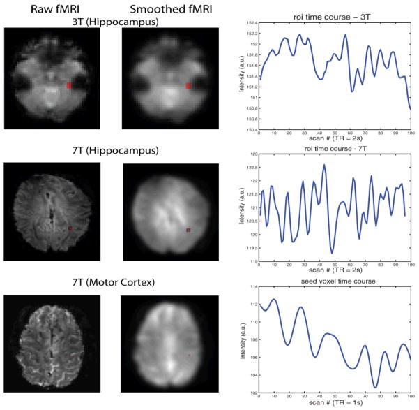
The 3T resting state fMRI image series (4×4×4 mm resolution, 46×55×46 voxels, TR = 2000 ms, 200 volumes) were analyzed through slice timing correction, realignment, co-registration, normalization, smoothness in SPM 8, followed by the time series low pass filter with a cut off frequency equal to 0.1Hz. A right hippocampus mask defined by WFUpickatlas (http://fmri.wfubmc.edu/software/PickAtlas) was used to define the seed region and the average time series signal were calculated (Figure 1).
Figure 1.
Presentation of data and seed regions. The first column show one slice raw images with the seed region marked in red for each data set. The second column displays the smoothed images. Note that we analyzed the smoothed images for hippocampus seed region but un-smoothed images for motor cortex seed voxel. The third column plots the average seed region intensity after preprocessed across the first 100 scans.
The 7T (Hippocampus) resting state MRI dataset (2×2×2 mm resolution, 96×96×12 voxels, TR = 2000 ms, 96 volumes) was analyzed to compute a connectivity map of the right hippocampus as the 3T fMRI (Figure 1). An image based physiological noise reduction method [15] was first applied to adjust physiological noise. Then a standard preprocessing containing slice timing correction, realignment, smoothness and low pass temporal filter were performed.
The 7T (Motor Cortex) fMRI data (2×2×2 mm resolution, 96×96×13 voxels, TR = 1000 ms, 500 volumes) were preprocessed by slice timing, realignment, low pass temporal filtering, and linearly detrending. The global average brain intensity was used as a confounding regressor. One voxel inside the right motor cortex was selected as the seed voxel (Figure 1).
3.2 Whitening Residuals Distribution
In fMRI analysis, the weight matrix is estimated by ReML for the whole brain. To explore the Gaussian assumption of the whitening data we calculated the residuals of the filtered weighted data. i.e., for each voxel
| (7) |
| (8) |
| (9) |
Where W is the weighted matrix used to whitening data, which is the same for every voxel, filter represents applying the filter specified in the 1st level fMRI design. Y is the fMRI image intensity, X is the design matrix, β is the estimated parameters calculated by SPM 8. ε is the residual that is assumed to be distributed as normal distribution.
For each resting state fMRI dataset, we calculated the kurtosis of the residuals across time in every brain voxel to compute a kurtosis map. The estimator of the popular kurtosis is defined as
| (10) |
where k4 is the unbiased estimator of the fourth culminant and k2 is the unbiased estimator of the population variance. It is an unbiased estimator of the population kurtosis that equals 0 for the normal distribution.
3.3 Robust fMRI Connectivity Analysis
Our robust estimation EM algorithm proposed in section 2 was tested as a preliminary robust method on our three datasets. It is implemented in SPM 8 by changing ordinary least squares regression to robust regression and applying weights in restricted maximum likelihood estimation. The resting state fMRI images are analyzed under the robust method and compared with the results acquired earlier.
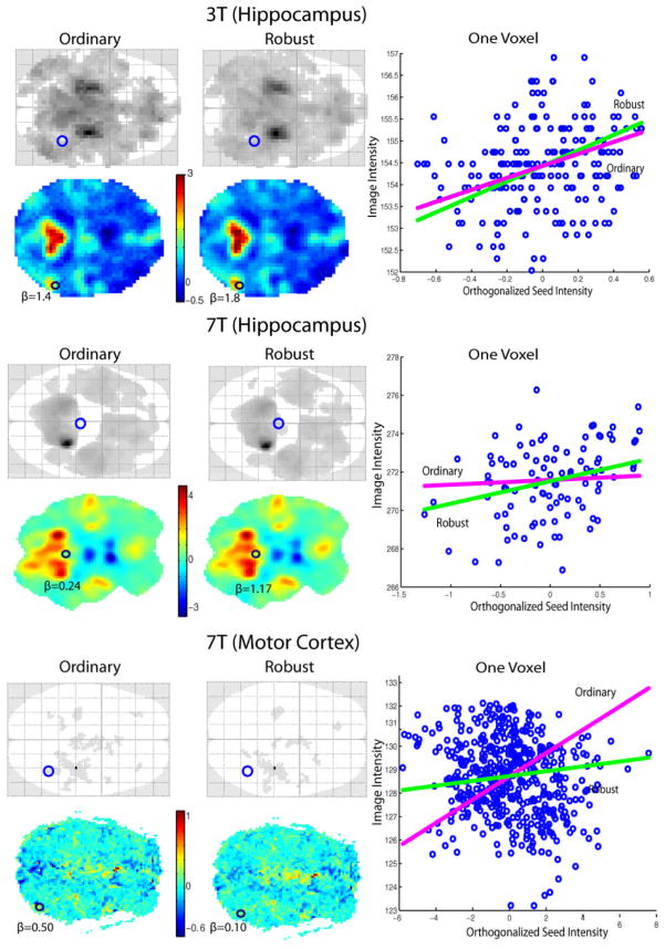
Images are processed as stated before, only the estimation method changes. One voxel which shows different significance result in the connectivity map estimated from the robust method and the ordinary method was studied. We plotted the raw data and the regression lines for the seed course ignoring the motion confounds. The seed intensity is the intensity after orthogonalized with respect to its mean and the motion parameter while the image intensity is from fMRI images after preprocessed.
4. RESULTS
The connectivity maps are displayed in Figure 2 in glass brains with one slice image overlapped. The statistical significance was calculated based on the 0.05 Family Wise error (FEW) p-value threshold and then projected to three dimensions. The results are shown with 10 voxels extent threshold to exclude noise. The darkest region represents the most correlated voxels to the seed region time series. We can expect that the most correlated voxels are inside the seed region. In the 3T fMRI connectivity map, the right hippocampus and the left hippocampus are much more significant than other regions. The right hippocampus region is also very significant in the 7T connectivity map, but the left hippocampus region is not as significant as we see in the result of the 3T fMRI dataset. The right motor cortex seed voxel of the 7T fMRI data is extremely significant since an orthogonalized time course is always perfectly correlated to itself and the extra motion regressors are not confounds. Bilateral correlations on each central sulcus are observed in the connectivity map as expected.
Figure 2.
Connectivity maps. The connectivity maps from fMRI analysis are shown in the glass brain projecting the significant voxels to three dimensions. The statistical significance is calculated based on corrected FWE p<0.05 and 10 voxels extent threshold to exclude noise. One slice image overlapped with the connectivity map is displayed following the glass brain.
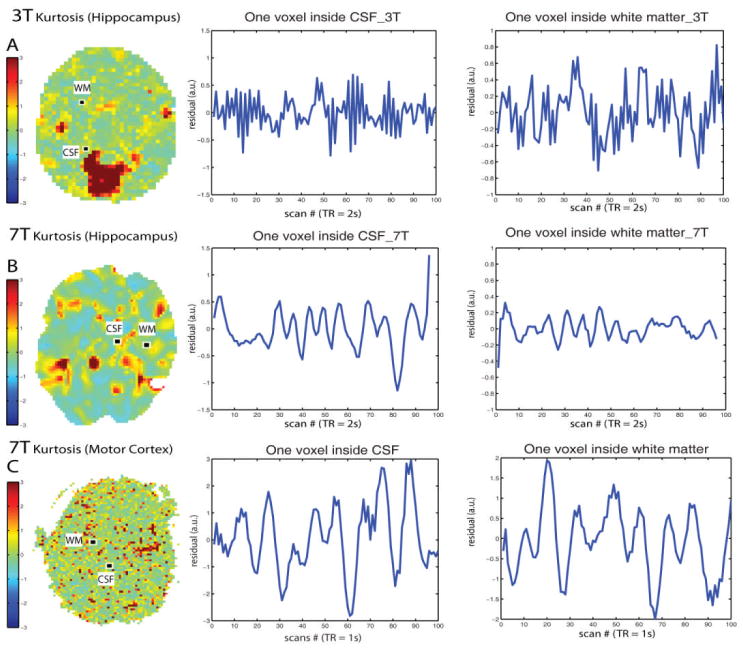
The kurtosis maps are shown in Figure 3 along with the plots of two selected voxel residuals across scans. The kurtosis values are randomly distributed in both 3T resting state fMRI and the 7T resting state fMRI with right motor cortex seed voxel. It confirms the assumption that the whitening resting state fMRI data are independent. However, the kurtosis maps of the 7T fMRI with right hippocampus exhibited spatial dependence.
Figure 3.
Kurtosis of weighted residuals. The Kurtosis maps of the residuals from the weighted data are shown in the first column. The middle and the right column display one voxel residuals across the first 100 scans inside the cerebrospinal fluid region and the white matter region respectively.
To explore the performance of our robust method on the resting state fMRI data, we compared the results from robust and non-robust fMRI analysis. The glass brains and the estimated parameters for the seed signal are compared in the Figure 4. The connectivity map estimated by the robust method seems getting more power and accuracy.
Figure 4.
Comparison of Ordinary and Robust methods. For each data set, the first left row displays one dimension glass brains of the connectivity maps based on corrected FWE p<0.05 and 10 voxels extent threshold to exclude noise. One slice of the estimated parameters for the seed signal from both ordinary and robust methods are shown in the second left row. One voxel inside the regions where the two methods estimated different significance is enlarged in the right column, which is corresponding to the blue circle in the glass brains and the black circle in the β images. The blue dots represent the raw data intensity. The seed intensity regression lines from ordinary and robust methods are plotted ignoring motion confounds.
5. DISCUSSION
In summary, we extend the robust estimation approach for autoregressive models and evaluated the qualitative impacts of this technique relative to traditional inference. Clear differences in statistical significance are shown between inferences based on classical versus robust assumptions, which suggest that inferences based on Gaussian assumptions are subject to practical (as well as theoretical) concerns regarding their power and validity. Hence, modern statistical approaches, such as the robust autoregressive model posed herein, are appropriate and suitable for inference with ultra-high field functional magnetic resonance imaging.
Acknowledgments
This project was supported by NIH N01-AG-4-0012. This work described herein has not been submitted elsewhere for publication or presentation.
References
- 1.Friston K, Jezzard P, Turner R. Analysis of functional MRI time series. Human Brain Mapping. 1994;1(2):153–171. [Google Scholar]
- 2.Friston K, Holmes A, Poline J, et al. Analysis of fMRI time-series revisited. Neuroimage. 1995;2(1):45–53. doi: 10.1006/nimg.1995.1007. [DOI] [PubMed] [Google Scholar]
- 3.Van Den Heuvel MP, Hulshoff Pol HE. Exploring the brain network: a review on resting-state fMRI functional connectivity. European Neuropsychopharmacology. 2010;20(8):519–534. doi: 10.1016/j.euroneuro.2010.03.008. [DOI] [PubMed] [Google Scholar]
- 4.Cole DM, Smith SM, Beckmann CF. Advances and pitfalls in the analysis and interpretation of resting-state FMRI data. Frontiers in systems neuroscience. 2010;4 doi: 10.3389/fnsys.2010.00008. [DOI] [PMC free article] [PubMed] [Google Scholar]
- 5.Hutchison RM, Leung LS, Mirsattari SM, et al. Resting-state networks in the macaque at 7 T. Neuroimage. 2011 doi: 10.1016/j.neuroimage.2011.02.063. [DOI] [PubMed] [Google Scholar]
- 6.Triantafyllou C, Hoge R, Krueger G, et al. Comparison of physiological noise at 1.5 T, 3 T and 7 T and optimization of fMRI acquisition parameters. Neuroimage. 2005;26(1):243–250. doi: 10.1016/j.neuroimage.2005.01.007. [DOI] [PubMed] [Google Scholar]
- 7.Hutton C, Josephs O, Stadler J, et al. The impact of physiological noise correction on fMRI at 7T. Neuroimage. 2011 doi: 10.1016/j.neuroimage.2011.04.018. [DOI] [PMC free article] [PubMed] [Google Scholar]
- 8.Diedrichsen J, Shadmehr R. Detecting and adjusting for artifacts in fMRI time series data. Neuroimage. 2005;27(3):624–634. doi: 10.1016/j.neuroimage.2005.04.039. [DOI] [PMC free article] [PubMed] [Google Scholar]
- 9.Huber PJ. Robust estimation of a location parameter. The Annals of Mathematical Statistics. 1964:73–101. [Google Scholar]
- 10.Holland PW, Welsch RE. Robust regression using iteratively reweighted least-squares. Communications in Statistics-Theory and Methods. 1977;6(9):813–827. [Google Scholar]
- 11.Gill PS. A robust mixed linear model analysis for longitudinal data. Statistics in medicine. 2000;19(7):975–987. doi: 10.1002/(sici)1097-0258(20000415)19:7<975::aid-sim381>3.0.co;2-9. [DOI] [PubMed] [Google Scholar]
- 12.Friston KJ, Glaser DE, Henson RNA, et al. Classical and Bayesian inference in neuroimaging: applications. Neuroimage. 2002;16(2):484–512. doi: 10.1006/nimg.2002.1091. [DOI] [PubMed] [Google Scholar]
- 13.Friston KJ, Penny W, Phillips C, et al. Classical and Bayesian inference in neuroimaging: theory. Neuroimage. 2002;16(2):465–483. doi: 10.1006/nimg.2002.1090. [DOI] [PubMed] [Google Scholar]
- 14.Neal RM, Hinton GE. A view of the EM algorithm that justifies incremental, sparse, and other variants. Learning in graphical models. 1998;89:355–368. [Google Scholar]
- 15.Glover GH, Li TQ, Ress D. Image based method for retrospective correction of physiological motion effects in fMRI: RETROICOR. Magnetic Resonance in Medicine. 2000;44(1):162–167. doi: 10.1002/1522-2594(200007)44:1<162::aid-mrm23>3.0.co;2-e. [DOI] [PubMed] [Google Scholar]


