Simple neural networks for the amplification and utilization of small changes in neuron firing rates

Abstract

I describe physiologically plausible “voter-coincidence” neural networks such that secondary “coincidence” neurons fire on the simultaneous receipt of sufficiently large sets of input pulses from primary sets of neurons. The networks operate such that the firing rate of the secondary, output neurons increases (or decreases) sharply when the mean firing rate of primary neurons increases (or decreases) to a much smaller degree. In certain sensory systems, signals that are generally smaller than the noise levels of individual primary detectors, are manifest in very small increases in the firing rates of sets of afferent neurons. For such systems, this kind of network can act to generate relatively large changes in the firing rate of secondary “coincidence” neurons. These differential amplification systems can be cascaded to generate sharp, “yes–no” spike signals that can direct behavioral responses.

The behavior of elasmobranchs (sharks, skates, and rays) is affected dramatically by very small electric fields in their pelagic environment (1). Those fields are known to change the electrical potential across the apical membranes of large numbers of detector cells in the ampullae of Lorenzini of the animals. These added potentials, as small as ΔV_m ≈ 200 nV, generate small changes in the firing rates of the afferent nerves that serve those cells (2–4) and the animal makes use of these small changes to determine his behavior.

The signal to any one detector element is very small compared with noise. Assuming that the signal acts by changing the opening probability of voltage-gated ion channels in the apical membrane of the cells and the effective gating charge is q_g = 6e, characteristic of the Hodgkin–Huxley model (5), the threshold signal energy for one channel is, dw = ΔV_mq_g ≈ 5 ⋅ 10⁻⁵ kT. Although the accompanying noise probably plays a significant role in amplifying the signal-to-noise (S/N) ratio somewhat as described by stochastic resonance arguments (6, 7), the effective S/N ratio is still quite small. However, there are many voltage-gated channels in each detector and large numbers of detector cells lining the ampullae, hence the overall S/N ratio can exceed 1.

Although the elasmobranch systems constitute the paradigmatic example inferentially addressed by this report, other sensory systems are known with similar sensitivities that may generate similar primary information. In the warmth–cold sensor system of mammals, changes in temperature as small as ΔT = 0.02 K (thus ΔT/T ≈ 1/15,000) generate small changes in the firing rates of two sets of sensory neurons—a warmth-sensing set and a cold-sensing set—that lead to behavioral modifications (8–10).

Also, honey bees make use of 100-nT variations in the magnetic field to map the position of food sources (11, 12). It seems that the fields generate forces on magnetosome elements (biological magnetite domains) held in hairs on the abdomen. On a small change in the ambient magnetic field, each of these elements presumably generates a small signal, perhaps by changing the firing rates of afferent neurons that serve hair-cell-like detector elements. The energies for so small a field acting on one detector seem likely to be small compared with kT, but there are probably many tens of thousands of detectors.

Hence, in each of these three paradigmatic systems, it seems that signals that involve energy transfers to the sensory elements that are much smaller than the basic thermal energy, kT, generate small changes in the firing rates of primary neurons. These rates are processed, somehow, so as to generate behaviors that must derive from some final, definite, “yes” or “no” neural signal. I describe biologically plausible neural network structures that might serve to take such small changes in firing rates and generate definite binary decision signals.

An Elementary Voter-Coincidence Network

I consider a set of N primary “detector” neurons, n₁, n₂, n₃, . . . n_N with a mean firing rate of ω_p action pulses per second (pps) but different individual firing rates, ω_j, where the rates are modified by stochastic effects so that the interval between pulses varies irregularly. These may be primary sensors themselves, as is the case for the warmth–cold systems, or afferent neurons that serve primary sensor cells that generate graded responses and do not, themselves, produce action pulses. Adair et al. (4) have suggested that the elasmobranch sensory neurons generate action pulses, a hypothesis that allows better fits to some data (13), whereas A. J. Kalmijn (23) has emphasized the possibility that the sensory cells generate a graded response as do the phylogenetically related mammalian hair cells.

The positive voltage pulses that are the outputs of these primary elements, uncorrelated in time, are fed in parallel into a “coincidence” neuron presumably through axon-to-dendrite synapse structures as suggested by the cartoon diagram of Fig. 1. (This is akin to a two layer perceptron with the input taken implicitly.) Those structures attenuate the voltage signals so that the voltage impulses passed to the coincidence neuron have different amplitudes, v_j, manifest as depolarization potentials. These neurons fire when the sum of the small incoming signals (from the voters) that are received in a characteristic resolution time Δt (the coincidence) exceeds a threshold value, ∑v_j > S. Measured as a depolarizing transmembrane potential, for Na⁺ channels described by Hodgkin–Huxley dynamics that threshold is (14) S ≈ 7 mv, but I do not use that number specifically in these calculations. As a consequence of various noise sources, the threshold, S, is assumed to vary stochastically over a small range. I show that under these realistic conditions, small changes in the mean firing rates of the detector cells will generate much larger changes in the firing rate of the coincidence cell.

Figure 1.

A schematic diagram suggesting the connections for a two-layer neuron network such that the firing rate of a secondary, coincidence neuron will vary proportionately more than the variance of a set of primary neurons. The input dendrite structures to the primary neurons may be absent when those neurons act as the sensory detector elements, as is the case for the warmth–cold systems (8).

A Toy Coincidence Model.

To provide insight into the character of the realistic model, I consider a “toy” model where certain simplistic simplifications are imposed. In particular, I assume that the mean firing rate of each of the N primary elements is equal to ω_p pps, although the pulses are emitted randomly in time. Further, I take the amplitudes of the signals received by the coincidence element as identical and equal to v. Then I assume a definite threshold of S = Mv taken over a resolution time, Δt, for the generation of action pulses where M is an integer.

With these assumptions, the mean number of signals arriving at the coincidence element in a time Δt will be ɛ = Nω_pΔt. The coincidence neuron will fire when k ≥ M signals arrives in the interval Δt. That probability is expressed by the Poisson relation,

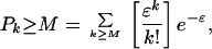1

where ɛ = Nω_pΔt is the mean number of signals received in the characteristic time, Δt, and the firing rate of the secondary coincidence neuron will be ω_V = P_k ≥ M/Δt.

For such a Poisson process (15), the proportional increase in the secondary (output) frequency, ω_s, will be much greater than that of the primary (input) frequency, ω_p. For a biologically interesting set of numbers—e.g., n = 50, ω_p = 30 pps, M = 12, and Δt = 5 ms—the multiplication factor,

2

A Realistic Model.

The properties of the toy model follow largely from the character of the Poisson distribution. Given a mean value of a random variable, the probability of a value larger than a threshold value that is itself significantly larger than that mean is dominated by the strong dependence of the Poisson distribution on that threshold. Thus, the introduction of further random variation might not be expected to modify the results of the simple toy model very much. Although the general tenor of more realistic models is then strongly suggested by such general arguments, it seems important to address the subtleties of reality by a model that encompasses more realistic constraints.

Although the model I use might reasonably be considered a stochastic version of the McCulloch–Pitts (16) model, it is arguably closer to biology, if less suited to formal analysis. Although the model is properly defined by the computational Monte Carlo program used to derive its properties, I will describe it in physiological terms both to make it more accessible and to better define its special characteristics and limitations.

I assume, first, that each member of a set of N_p primary sensor neurons generates action potentials (spikes) that feed into a secondary coincidence neuron. Stochastic noise seems to play a key role in amplifying the sensitivity of the primary sensory detectors (6). That noise, derived especially from shot noise in the pumping and leakage currents that set resting potentials and in the chatter of channels opening and shutting, is reflected in variations in the firing periods of the primary sensory elements and/or in the periods of the afferent nerves that serve primary elements that generate graded responses. Hence, I take it that each individual primary neuron, j, fires with a given probability, p_j, per unit time. In general, the primary elements will differ as a consequence of general biological diversity and will emit action pulses at different frequencies. This is especially evident in the large differences between individual cold-sensing neuron fibers (17) and between different warm sensing fibers (18). Hence, I take the individual frequencies as, ω_j ≈ 1/p_j, where the firing probabilities, p_j, are to be distributed about a central probability, pP = 1/ω_p, in a normal distribution with a standard deviation of p_p/2. I also assume a refractory dead-time after each pulse of 3 ms and adjust the firing probabilities so as to generate the assigned frequencies.

I assume that the signal that reaches the secondary neuron is attenuated variously by the transmission through primary axons and secondary dendrites. Synapse inefficiencies also act so as to reduce the effective signal strength of the input neurons. Although individual synapse efficiencies can be less than 0.5, the axon-to-dendrite connection can involve several synapses, thus increasing the overall efficiency. To simulate such differences, I assumed that the received signal strengths vary about normally about a central value, v_p, with a standard deviation of σ_v = v_p/4.

In these calculations I assumed, implicitly, rather small synapse inefficiencies, the effects of which are presumed to be reflected in the variation of the effective frequencies of the input neurons. If the synapse inefficiencies are large—e.g., >0.5—the specific calculations shown here may not apply, although the general tenor of the model should still obtain.

I take the signal as effecting a depolarization potential in the secondary neuron proportional to the signal amplitude and consider that the depolarization dissipates with a “pulse-length” relaxation time constant, τ. Implicitly, I treat the incoming spike signal as short—no greater than the 1-ms time-slices used in the numerical computation. However, the results are not much changed as long as the spike duration is shorter than τ.

I then assume that the secondary, coincidence neuron will fire when the average incremental depolarization voltage, V(t), taken over an integration time Δt, exceeds a threshold potential, S. That potential derives, in turn, from the summed input of the N_p primary neurons over time where that depolarization voltage decays with the pulse-length time, τ. Thus the condition for a spike generation is,

3

where v_j is the magnitude of the depolarization pulse from the primary neuron, j. In the actual calculation, I use 1-ms time-slices, the time-integrals are then approximated by appropriate summations and I take the trigger time, Δt = 1 ms or one time-slice. After every secondary spike, I introduce a secondary refractory dead time of 3 ms.

At this point, after a secondary output spike, I calculate two refractory variations: (i) I leave the V(t′) untouched and (ii) I reset the “depolarization potential,” V(t′) in Eq. 3, to zero. Of course, realities can be expected to be richer yet in variations.

Even as the occupation of different states—open and closed—of the ion channels is subject to thermal noise fluctuations the trigger process and trigger potential can be expected to vary to some extent. To simulate this variance I inject noise into the secondary firing process by varying the threshold every ms taking the values as distributed normally about the primary value, S, with a standard deviation of σ_S = S/10. That threshold is defined in units of v_p such that no assignment of absolute values for either S or v_p is necessary.

By comparing the arithmetic sum of the input pulses with the threshold, I implicitly assume a linear response to the input pulses. Although for very small pulses a linear response is likely (19), for the accumulation near the thresholds some deviation from linearity can be expected. (Of course, the spike action that follows from the threshold crossing is quite nonlinear.) Qualitatively, the arguments hold for almost any monotonic variation of the response to the input and modest variances from linearity do not affect the character of the results stated here.

Even as the secondary firing rates vary sensitively with the primary rates, the secondary rates are sensitive to any variation of the central threshold value, S, which must, then, be held within narrow limits if the system is to operate effectively. Such a threshold must also adapt to long-term physiological changes. Adaptation mechanisms that will handle such variations operate in other modalities (8, 14) and I postulate that such mechanisms operate in coincidence neurons.

Sensitivities.

In the numerical Monte Carlo calculations, the incoming pulses from each primary element were recorded, or not recorded, by chance for each millisecond time-slice, according to probabilities defined by their firing rates. The sum of these stochastically determined intensities was than compared with the coincidence threshold, S, and if that sum exceeded S, an output action pulse was recorded.

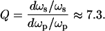
Using this “realistic model,” the coincidence firing rate, ω_j, was calculated by Monte Carlo techniques as a function of the “primary” rate for sets of 25, 50, and 100 primary cells feeding into one coincidence neuron. Although the results specifically discussed here follow from the choice of ω_p = 30 pps as the central primary frequency, taken to be near that recorded for afferent nerves serving the primary detectors of skates (2), qualitative similar conclusions also hold for other choices of the central frequency.

Fig. 2 shows the calculated gain factors, Q, for the two secondary spike refractory models, as a function of the number of primary elements and effective primary pulse lengths where the central primary frequency ω_p = 30 pps and the secondary frequency is also held at ω_s = 30 pps. Calculations made with other values of ω_s showed that for either model variant, Q was insensitive to the choice of the central secondary frequency made although changes in the threshold, S. For the first (no reset) model variant, the gain increases with an increase in the number of primary sources and with the pulse length. As these quantities increase, the number of contributions from incoming pulses that are required to exceed the threshold increases (as ɛ in Eq. 1), thus generating an increase in sensitivity. For the second (reset) model variant, Q decreases with increasing pulse length for lengths greater than the 3-ms secondary spike refractory period that was introduced even as after a such pulse the sum of the extant pulses is reduced to zero and the build-up toward the trigger point must begin anew.

Figure 2.

The frequency multiplication factor, Q, as derived from Monte Carlo calculations, taken as a function of primary pulse length for 25, 50, and 100 primary elements feeding into a coincidence neuron. The solid lines show the values for the no reset model.

In my presentation of the results shown in Fig. 2, I have limited the range of pulse lengths, τ, to those such that ωτ < 1/3, where ω is either the primary or secondary frequency. That product is a measure of the portion of time the element is in a refractory state and for larger values of that product the conclusion are excessively sensitive to assumptions concerning the firing mechanisms of the neurons, which I prefer to avoid.

Output Noise.

Even as the properties of the output of the secondary coincidence neuron follow from the random character of the input, the secondary output is also random. For any time period that is long compared with the output neuron spike refractory period taken as 3 ms, the number of spikes varies as a Poisson distribution about the mean number. (The generation of spikes from the secondary coincidence neuron is then a Poisson process, though the production of primary spikes may be less random.) As a consequence of the random generation of secondary spikes, the secondary output from a set of primary neurons can serve as a primary input to a tertiary coincident neuron in this scheme.

Input Noise.

Although the random character of the received primary pulses plays an essential role in the networks discussed here, the magnitude of the noise does not. A relaxation of the variances introduced in the model does not much compromise the model. In particular, by direct calculation the multiplication factor Q was shown to be little affected by a reduction of the random variation in every physiological and stochastic parameter by a factor of 3. It seems that as long as the variation in the periods between pulses from the different primary sources is not much smaller than the secondary neuron integration time, set here as 1 ms, Q is not much affected by the magnitude of the noise.

Indeed, in general the model is extraordinarily robust, demanding little in the way of any conformation to specifics by nature.

S/N Discrimination.

For the primary elements used in the specific calculations presented here, the mean number of spikes emitted in a period, dt, will be NP = ω_pdt, where the mean frequency of the primary elements is ω_p and the integration time is dt. For this discussion I assume a normal distribution of the number of spikes in an interval such that the standard deviation is σ_p ≈ = . For the elasmobranch signals, the noise is not well known but may be somewhat less than that calculated by the above recipe (2, 4).

A single network consisting of a set of primary neurons and a secondary neuron then loses information. Approximating the deviance of the number of primary output pulses over a period Δt as σ ≈ ω_pΔt, characteristic of a Poisson process, and taking the multiplication factor of the coincidence system from Fig. 2 (and Eq. 2) as Q ∝ 0.42N, where N_p is the number of primary elements, Q increases less with the number of primary detectors, N_p, than Q′ ∝ expected if the information from the primary array were used efficiently.

For some models, the deviance of the primary output is appreciably less than from a Poisson model and the information loss is then more drastic. (In their model of detector cell spike production in elasmobranch electric field detection, which they consider realistic, Adair et al. (4) find that the detector neurons have, effectively, a long refractory period that reduces their deviance to about 10% of that for a Poisson process.)

Extensions: Cascade, Yes–No, and Differential Networks

Cascade Networks.

Further layers of voter-coincidence arrays, as suggested by the diagrams of a miniature three-layer system in Fig. 3, can sharpen discrimination. Here eight primary elements each feed two of the four secondary elements, which in turn feed one tertiary element. With larger numbers, such cascading generates a strong multiplication factor, Q, for a given number of neurons.

Figure 3.

Diagram of a three-layer system (with the inputs suppressed) showing schematically a miniature neuron network where eight primary neurons (1) feed four secondary neurons (2) that, in turn, feed a tertiary neuron (3).

It is useful to apply the cascade model to the estimation of the S/N in the elasmobranch system to demonstrate that the cascade model is roughly adequate to explain the observed sensitivity of the fish. For a least-detectable signal, I take the membrane potential deviation as ΔV_m = 100 nV (1, 3, 14) and the signal applied to a single voltage gated calcium ion channel as S₁ = 6e ⋅ ΔV_m. Assuming thermal noise and N₁ = kT, S₁/N₁ = S₁/kT ≈ 2.5 ⋅ 10⁻⁵, where k is Boltzmann's constant and T the Kelvin temperature. If the area of the apical membrane is 100 μm² and the density of channels is 450 per μm², for the whole sensor cell, S_c/N_c ≈ 2.5 ⋅ 10⁻⁵ × ≈ 0.005 for the cell with 45,000 channels.

Taking the rate of increase of the neuron firing rate with the incremental membrane voltage as (dω/ω)/dV_m ≈ 0.03/μV (2, 4), the 100-nV threshold signal would cause a change of about Δω_p/ω_p ≈ 0.003 or about 0.1 pps in the 30 pps normal firing rate of the cell. Choosing a signal duration of Δt = 100 ms as a plausible fish reaction time, the S/N for one sensor cell will be S/N ≈ Δω_p ≈ 0.006.

Then 50 such elements, servicing a secondary coincidence neuron operating such that the multiplication factor is 7, will generate a spiking frequency change of 2% from that secondary cell. If 50 such secondary neurons (and thus 2,500 primary neurons) feed a tertiary coincidence neuron, also with a gain of Q = 7, the original signal will cause the spike frequency of that neuron to change by about 14%. The ratio S/N ≈ 0.25 will still be less than one. But if 50 tertiary neurons feed one quartiary neuron, again with a gain of 7, we can expect that S/N ≈ 1.7 and that a reasonably clean signal will emerge. Thus, 125,000 primary sensory neurons can be processed to generate a definite discrimination in a period of less than 100 ms.

Hence, with but one connection per unit to the higher array, this system would require ≈10⁵ cells to produce a distinctive signal in 0.1 seconds. But for an ideally efficient system S/N ∝ and only about 5,000 primary detector cells would be needed to gain the same S/N. For cascaded systems, under ideal conditions, where the final efficiency is still appreciably less than one, that efficiency will vary as the square root of the number of secondary elements fed by an average primary element. Hence, if each primary detector feeds many secondary neurons and each of these feeds many tertiary neurons, a reduction to as few as 25,000 elements seems in reach.

Although more complex networks might require only 5,000 primary elements to achieve the same S/N, the organism may, through evolutionary imperatives, prefer to increase its sensitivity by increasing the number of detector elements rather than by constructing more efficient, but much more complex, information handling circuitry.

If the primary signals are wholly random—as in a Poisson process—S/N varies as the square root of the number of spike periods observed; but this, of course, requires long observation times to gain sensitivity. In the sensory systems that I have singled out as plausible candidates for this model—the detection of weak electric fields by elasmobranchs, the warmth–cold sensation in mammals, and the detection by bees of very small changes in the terrestrial magnetic field—the time constraint on the behavioral response is not likely to be severe. Applying this model to sharks, typically, four cascade layers servicing 100,000 primary detectors, with a total gain of, perhaps, 350, can operate in less than 1/10 of a second. With smaller signal transfer distances, bees may gain the same sensitivity in less time or, more likely, be able to use more amplification stages. Many fewer detector neurons contribute to the warmth–cold sensation, but the integration time is about 3 s (8, 10), giving a nominal improvement of about 5.5 in S/N over a 1/10-s observation time.

A cascade system will operate with several connections to the next coincidence level only if the nominal equivalence of the pulses sent by a primary to different detector elements is destroyed. In some circumstances, weak interactions—such as through gap junctions connecting geographic neighbors—between the neurons of such a set can induce a self-organization that results in correlations between the pulse generation times of members of the set (4). Even if such strong correlations are absent, if two nearly equivalent secondary detectors receive the same incoming pulses from the same set of primaries, their secondary pulses will be highly correlated. That correlation will be reduced by the stochastic noise variation in thresholds, by differences in the incoming pulses that follow different axon–dendrite paths connecting each primary element to the different secondary elements, and by different synapse efficiencies for the different axon–dendrite connections. The different paths generate different attenuation factors and somewhat different time delays. The time delay differences are not likely to be more than a millisecond (14), but that difference might be sufficient to reduce the correlations to some extent. My numerical calculations have suggested that those secondary detectors that serve overlapping primary populations are effectively independent if those populations do not greatly overlap.

Although a final binary output that follows from a cascade of coincidence networks can lead to definite signals that derive from very small changes in the mean firing rates of primary neurons, the additional stages, each effected by thermal and other noise, can only increase the fundamental S/N ratio of the primary set. I have not been able to describe that increase analytically, but the results of numerical calculations suggest that, for practical systems, that increase is small and masked by the fundamental inefficiencies of the network design.

Yes–No Decisions.

If small changes in firing frequencies are to lead to behavior decisions, the logical chain of networks must terminate in a yes–no element. The voter-coincidence circuit can be used to transform a change in frequency to such a binary result. The diagram of Fig. 4 shows the output frequency as a function of input frequency for a voter-coincidence circuit with inputs of 25, 50, and 100 elements with 5- and 10-ms pulse lengths. The model i choice, with no reset of secondary potential, was used in the calculations, although the results are not highly sensitive to that choice. The sigmoid curves represent best fits of the function P(ω) = 1/(1 + exp{−aΔω}), to points generated by Monte Carlo calculations. Here P is the probability of the secondary element generating a spike in a 100-ms interval, Δω = ω − ω₀, where ω is the mean frequency of the primary input elements, ω₀ is the neutral frequency, and a is the steepness variable adjusted to generate a least-squares best fit.

Figure 4.

Probability of yes output spike indications (one or more output pulses) registered by a secondary coincidence in a 1/10-s interval for a neuron fed by 25, 50, and 100 primary neurons with pulse lengths of 5 ms and 10 ms. The threshold is set to generate 50% yes indications for primary counting rates of 30 pps. The curves represent the best least-squares fit to sigmoid functions described in the text to points generated through Monte Carlo calculations. The points are shown for the 50-counter results with a 10-ms pulse length to suggest the quality of the fit to the points.

Such a 100-element circuit processing 10-ms-long pulses will generate a spike in 1/10 s with a probability of 95% if the primary frequency is greater than 34 pps, but only 5% of the time if the primary frequency is less than 24 pps. A trigger rate greater than 39 pps will then generate a positive output more than 95% of the time, whereas rates less than 24 pps will give false positives less than 5% of the time.

Here I assume implicitly that, under appropriate circumstances, the information carried by one spike can lead to a definite decision (20) by the organism.

In this model, the yes–no system would be applied as a final stage after several stages of sensitivity amplification.

Differential Discrimination Networks.

An electric field to the left [right] of the swimming elasmobranch acts to increase the firing rate of the afferent nerves serving the sensory cells in the left-hand [right-hand] ampullae and decrease the rates in the nerves serving the right-hand [left-hand] ampullae. Because of the general symmetry of the animals, the base rates of the left and right sensory cells are likely to be very nearly the same, although both rates probably vary with temperature and that temperature will vary with the water temperature and with the different energy expenditures of the swimming fish. Hence, it is attractive to consider signal processing networks that are sensitive to changes in the difference between two input firing rates and are relatively insensitive to the mean rates.

In a somewhat similar pattern, a slight increase (decrease) in temperature decreases (increases) the firing rate of the cold-sensing sensory nerves in humans and other mammals, and increases (decreases) the firing rates of the warmth-sensing nerves. Again, networks that exploit the differences in the firing rates are attractive. Although the base firing rates for the warmth-sensing and cold-sensing sets of sensors seem to be about equal, the two sets differ greatly in their structure and in the number or density of elements, and differ somewhat even in their depth in the skin (8). Hence, any mechanisms that exploit the dual changes are likely to work on data from layers of processing that are quite different for the two modalities.

To exploit differences in firing rates, I suggest a coincidence–anticoincidence system where the elements from the set with increasing (or decreasing) firing rates are in coincidence, adding their inputs, while the elements from the set with decreasing (increasing) firing rates are in anticoincidence, subtracting their input amplitudes. I assume, in effect, that the pulses from the coincidence elements act to incrementally depolarize the cell and that the pulses from the anticoincidence elements act to incrementally hyperpolarize the cell.

In my calculations, excepting for the reversal of sign of the pulses from the anticoincidence entries, I use the same calculational procedures as described above for the coincidence network. Here I used the model i variant with no reset of the potential after a secondary pulse although the results were not sensitive to that choice. Again I take the positive, yes, output as one or more pulses in a 100-ms interval and select a threshold that generates a 50% positive response when the mean pulse rate for each primary element is 30 pps. Although the positive coincidence inputs and negative anticoincidence inputs are likely to have different properties (21, 22), the numerical results given here are for systems in which the relaxation time constants—pulse-lengths—are taken to be the same for the two kinds of input. However, as a consequence of the uncertain character of the approximations, the vernier model must be considered as suggestive rather than descriptive and the numerical results are meant only to suggest the general character of such models and to provide an estimate of simply achievable sensitivities.

Fig. 5 shows the rate of yes counts, so defined, as it varies with the difference in firing rate frequency of two equal sets of i elements where the mean rate of all elements is held at 30 pps. Again, the sigmoid curves of the form P = 1/(1 + exp{−a Δω}) represent best fits to points calculated by Monte Carlo methods. Here, Δω was the difference between the primary yes and no counting rates, P was the probability of generation of secondary spike in a 100-ms interval, and a was the steepness fit parameter.

Figure 5.

The yes probability, defined by the receipt of one or more output pulses in a 1/10 s-interval, from a vernier (coincidence-anticoincidence) network as a function of the frequency difference between two sets of primary elements, where each set consists of 100 yes (y) elements in coincidence and 100 no (n) elements in anticoincidence and sets of 50 y and 50 n and 25 y and 25 n elements. The curves represent the best fit to sigmoid functions described in the text to points generated through Monte Carlo calculations. The points are shown for the (25 y + 25 n) results to suggest the quality of the fit to the points. In each case, the primary pulse length was taken as 10 ms.

For 200 primary elements, 100 positive and 100 negative, with both effective pulse lengths of 10 ms, we can expect a yes count for about 90% of the 100-ms intervals if the mean positive input frequency is 6 pps greater than the negative input frequency. Conversely, if the negative rate is 6 pps greater than the positive rate, there will be a yes pulse only 10% of the time.

In nature, each set, plus or minus, will presumably be the result of a cascade of sets of coincidence elements that serve to multiply small variations of rates from very large numbers of sensory cells. Hence, the difference of 6 pps can be presumed to reflect a very much smaller frequency difference between two sets of basic elements.

However, because the biology of the depolarizing coincidence and the inhibiting anticoincidence (which I treat as a simple hyperpolarization) are in fact rather different and may not add arithmetically as I assume in the model, my symmetric linear treatment of the two inputs may not be very close to Nature in detail. However, I believe that the results shown in Fig. 5, and the numerical conclusions stated by using those results, are suggestive of the properties of possible real systems.

For symmetric systems such as that of the elasmobranchs, I would expect two (sets) of coincidence–anticoincidence networks operating with the coincidence and anticoincidence entries reversed. Then, with the result shown in Fig. 5 for 100 Y-counters and 100 N-counters, both with 10-ms-long pulses with frequencies differing by 6 pps, about 10% of the time there will be a false positive from the complementary set. Thus, for Δω = 6 pps, there will be a clear left–right signal about 81% of the time, an incorrect signal about 1% of the time, and an indeterminate signal (double positive or double negative) about 18% of the time.

At least for our paradigmatic elasmobranch sensory system, the coincidence neuron for the yes–no network need only have a sparse production of decision pulses. The spike that means “swim left” must be sent to trigger the neuron network in the central nervous system, which sends a properly timed set of pulses down long axons to the muscles that drive the fish through the water. All of this must take on the order of 100 ms. Thus, a set of “swim left” signals at a rate of 1 or more per 100 ms will quickly turn the fish. If there intrudes an occasional blank or absence of a signal, a confusing “swim right–swim left” signal, or even a rare erroneous “swim right” signal, there will be little disruption of the basic swim-left instruction and little harm.

Some systems may integrate signals. A 1/10-s integration time seems within our biological understanding of the time constants of different ion channels, and longer times do not seem unreasonable. I note again that the warmth–cold response threshold reaches a maximum sensitivity after about 3 s of exposure (8), which suggests an integration time of that magnitude.

Conclusions

Some sensory systems generate information in terms of small changes in the firing rates of afferent neurons where that rate is affected strongly by noise. If that information is to lead to a definite physiological or behavioral decision, the changes in the firing rates of many elements must be processed in a manner that amplifies the rate variation. Then, finally, that rate variation must be processed in a manner than generates a binary yes–no result.

I show that simple, physiologically plausible neural networks—where the neuron acts as a voter-coincidence element—can be constructed that amplify such firing rate variances for uncorrelated primary neurons. Then, the same kind of elements can be used in a further network element to produce the requisite binary yes–no output.

The proposed networks, constructed from generic neurons with generic properties, are robust; easily accommodating significant variations. Broadly speaking, they accept large sets of noisy uncertain information, which can be weighted, and derive from that information a definite binary, yes–no decision. Although the model networks introduced here are suggested as a mechanism to process certain sensory data, their generality suggests that such networks might be used also in other areas of the nervous system.

Abbreviations

pps

pulses per second

S/N

signal-to-noise

References

- 1.Kalmijn A J. Nature (London) 1986;212:1232–1233. [Google Scholar]
- 2.Lu J, Fishman H M. Biophys J. 1994;67:1525–1533. doi: 10.1016/S0006-3495(94)80626-5. [DOI] [PMC free article] [PubMed] [Google Scholar]
- 3.Pickard W F. IEEE Trans Biomed Eng. 1988;35:243–249. doi: 10.1109/10.1372. [DOI] [PubMed] [Google Scholar]
- 4.Adair R K, Astumian R D, Weaver J C. Chaos. 1998;8:576–587. doi: 10.1063/1.166339. [DOI] [PubMed] [Google Scholar]
- 5.Hodgkins A L, Huxley A F. Am J Physiol London. 1952;117:500–544. doi: 10.1113/jphysiol.1952.sp004764. [DOI] [PMC free article] [PubMed] [Google Scholar]
- 6.Astumian R D, Weaver J C, Adair R K. Proc Natl Acad Sci USA. 1995;92:3740–3743. doi: 10.1073/pnas.92.9.3740. [DOI] [PMC free article] [PubMed] [Google Scholar]
- 7.McNamara B, Wiesenfeld K. Phys Rev A. 1989;39:4854–4869. doi: 10.1103/physreva.39.4854. [DOI] [PubMed] [Google Scholar]
- 8.Hensel H. Monographs of the Physiological Society 38. London: Academic; 1981. [PubMed] [Google Scholar]
- 9.Kenshalo D R. In: Sensory Functions of the Skin in Primates. Zotterman Y, editor. Oxford: Pergamon; 1976. pp. 305–330. [Google Scholar]
- 10.Adair R K. Proc Natl Acad Sci USA. 1999;96:11825–11829. doi: 10.1073/pnas.96.21.11825. [DOI] [PMC free article] [PubMed] [Google Scholar]
- 11.Walker M M, Bitterman M E. J Comp Physiol A. 1985;57:67–73. [Google Scholar]
- 12.Kirschvink J L, Kobayashi-Kirschvink A. Am J Zool. 1991;31:169–185. [Google Scholar]
- 13.Clusin W T, Bennett M V L. J Gen Physiol. 1977;69:145–182. doi: 10.1085/jgp.69.2.145. [DOI] [PMC free article] [PubMed] [Google Scholar]
- 14.Koch C. Biophysics of Computation. New York: Oxford Univ. Press; 1999. [Google Scholar]
- 15.Siebert W M. Kybernetic. 1965;2:206–215. doi: 10.1007/BF00306416. [DOI] [PubMed] [Google Scholar]
- 16.McCulloch W S, Pitts W. Bull Math Biophys. 1943;5:115–113. [Google Scholar]
- 17.Hensel H, Wurster R D. Pflügers Arch. 1969;313:153–154. doi: 10.1007/BF00586243. [DOI] [PubMed] [Google Scholar]
- 18.Hensel H, Kenshalo D R. J Physiol (London) 1969;204:99–112. doi: 10.1113/jphysiol.1969.sp008901. [DOI] [PMC free article] [PubMed] [Google Scholar]
- 19.Adair R K. Proc Natl Acad Sci USA. 1994;91:9422–9425. doi: 10.1073/pnas.91.20.9422. [DOI] [PMC free article] [PubMed] [Google Scholar]
- 20.Rieke F, Warland D, de Ruyter van Steveninck R, Bialek W. Spikes: Exploring the Neural Code. Cambridge, MA: MIT Press; 1998. [Google Scholar]
- 21.Shepherd G M. Neurobiology. New York: Oxford Univ. Press; 1994. [Google Scholar]
- 22.Huguenard J, McCormick D A. Electrophysiology of the Neuron. New York: Oxford Univ. Press; 1994. [Google Scholar]
- 23.Kalmijn A J. Proc Trans R Soc London B. 2000;355:1135–1141. doi: 10.1098/rstb.2000.0654. [DOI] [PMC free article] [PubMed] [Google Scholar]