Angular versus spatial resolution trade‐offs for diffusion imaging under time constraints

Abstract

Diffusion weighted magnetic resonance imaging (DW‐MRI) are now widely used to assess brain integrity in clinical populations. The growing interest in mapping brain connectivity has made it vital to consider what scanning parameters affect the accuracy, stability, and signal‐to‐noise of diffusion measures. Trade‐offs between scan parameters can only be optimized if their effects on various commonly‐derived measures are better understood. To explore angular versus spatial resolution trade‐offs in standard tensor‐derived measures, and in measures that use the full angular information in diffusion signal, we scanned eight subjects twice, 2 weeks apart, using three protocols that took the same amount of time (7 min). Scans with 3.0, 2.7, 2.5 mm isotropic voxels were collected using 48, 41, and 37 diffusion‐sensitized gradients to equalize scan times. A specially designed DTI phantom was also scanned with the same protocols, and different b‐values. We assessed how several diffusion measures including fractional anisotropy (FA), mean diffusivity (MD), and the full 3D orientation distribution function (ODF) depended on the spatial/angular resolution and the SNR. We also created maps of stability over time in the FA, MD, ODF, skeleton FA of 14 TBSS‐derived ROIs, and an information uncertainty index derived from the tensor distribution function, which models the signal using a continuous mixture of tensors. In scans of the same duration, higher angular resolution and larger voxels boosted SNR and improved stability over time. The increased partial voluming in large voxels also led to bias in estimating FA, but this was partially addressed by using “beyond‐tensor” models of diffusion. Hum Brain Mapp 34:2688–2706, 2013. © 2012 Wiley Periodicals, Inc.

INTRODUCTION

High angular resolution diffusion imaging (HARDI) is one of several advanced diffusion weighted imaging techniques [Tuch et al., 1999, 2002, 2004; Wedeen et al., 2005] that can resolve complex diffusion geometries, such as fiber crossings and intermixing of white matter tracts in the brain. In regions where fibers cross, the standard single‐tensor model (used in diffusion tensor imaging; DTI) is misleading; measures of fiber integrity, such as the fractional anisotropy (FA), tend to be underestimated, and fiber orientations are poorly approximated by the fitted tensor. Increasing the number of diffusion‐sensitive directional gradients can improve the accuracy of recovered white matter fiber‐tract orientations, as can increasing the spatial resolution; but each of these adds to the scan time. Several major initiatives, such as the NIH‐funded “Human Connectome Project,” are now devoted to understanding factors that affect brain integrity and connectivity [e.g., genetic versus environmental factors, sex differences, and maturation; Chiang et al., 2010 ; Jahanshad et al., 2011; Lepore et al., 2010; Zhan et al., 2010a]. Many efforts also combine diffusion imaging with resting‐state functional MRI or EEG/MEG to examine intrinsic functional correlations in brain activation, and how it relates to anatomical connectivity [Sporns, 2010; Wagner and Fuchs, 2001]. These efforts make it increasingly important to understand how DTI scanning parameters affect the results, and what trade‐offs are reasonable when scan time is limited.

Generally, when patients or healthy volunteers participate in large‐scale imaging studies, such as the Alzheimer's Disease Neuroimaging Initiative (ADNI; http://adni.loni.ucla.edu/), several structural and functional MRI sequences need to be completed, often within less than an hour. Several MRI scanning techniques are often combined to assess multiple candidate biomarkers of a disease, or to map brain connectivity. To limit patient discomfort, and avoid patient attrition (failure to complete the scan, or failure to return in a longitudinal study), trade‐offs must be made between angular and spatial resolution to obtain the best image quality in an acceptable time.

Prior studies describe several procedures to boost the signal‐to‐noise ratio (SNR) in diffusion imaging through lengthy imaging sessions, extensive q‐space sampling (including scans at multiple different b‐values), or diffusion spectrum imaging [Jones et al., 2004; Tuch 2004; Wedeen et al., 2005, Zhan et al., 2010c, 2011]. These may be ideal for research purposes [Liu et al., 2010], but most large‐scale clinical diffusion weighted imaging protocols are part of a session that includes several imaging series, leaving only a limited time for each scan. Limiting the time for diffusion weighted imaging limits the number of achievable applied directional gradients and also limits the spatial resolution of the images. Our prior studies created reference curves showing how the number of diffusion directions acquired affects the SNR for various standard DTI‐derived measures [Zhan et al., 2009a, 2009b]. Others have studied how the scanning protocol affects reconstruction errors in the principal eigenvector field, which is important for tractography as it determines the directions of the reconstructed fibers [Landman et al., 2007]. Even so, no studies, to our knowledge, have examined the trade‐offs between spatial and angular detail for estimating HARDI derived measures such as the Orientation Distribution Function (ODF), which we also assess here.

Information on signal reproducibility is also important. Smaller voxels (finer spatial resolution) may lead to higher mean differences in the DTI‐derived measures over time, due to the poorer SNR. Larger voxels, in general, offer greater longitudinal stability, although the resulting measures may be biased or have greater errors due to partial volume averaging. In two recent reports [Jahanshad et al., 2010, 2012a], we began to study how scan protocols affect the reproducibility of DTI measures over time. We only focused on standard DTI‐derived measures, such as the fractional anisotropy (FA) computed from the diffusion tensor. Although this is perhaps the most widely used measure of fiber integrity, more sophisticated models of diffusion geometry can estimate more detailed fiber directions, avoiding bias in estimating fiber anisotropy. Here we extend our earlier work to examine how diffusion related measures depend on the scanning protocol.

In this study, we investigated trade‐offs in angular and spatial resolution for three 7‐min protocols, which were candidates for use in the second phase of ADNI. We assessed how the protocol affected several widely used measures including: fractional anisotropy (FA), mean diffusivity (MD), and the HARDI‐derived ODF. We hypothesized that (1) larger voxels would boost the SNR and allow for more detailed angular sampling during a fixed scan time, and (2) a “beyond‐tensor” model (i.e., a more complex model than fitting a single tensor to the diffusion data) would help avoid partial volume effects, which can be a serious problem in large voxels. We also performed computational simulations to create data with prescribed fiber parameters, crossings, and noise, to reveal how scan parameters (e.g., voxel size) affect the derived DTI measures. Clearly, the “best” DTI protocol depends on whether a project aims to assess anisotropy or connectivity or both, and what levels of accuracy and reproducibility are both desirable and achievable, given the constraints. As such, we aimed to develop some general principles based on studying these trade‐offs empirically.

METHODS

Subjects and Image Acquisition

Eight healthy subjects (age: 32.0 ± 3.9 yrs SD; 4 male; 7 right‐handed) were scanned using a GE 3 T brain MRI scanner, with an 8‐channel head coil, running 14.0 M5 software. To explore trade‐offs between spatial and angular resolution, we used three separate scanning protocols, each with an overall acquisition time held fixed at 7 min ± 3 seconds. For each image series, there was an additional EPI calibration scan lasting ∼ 1 min. These tests were part of a preparatory phase of the Alzheimer's Disease Neuroimaging Initiative, in which different protocols were compared for their stability and signal‐to‐noise, within the constraints that (1) they could be readily implemented on a large number of scanners (15 sites) across North America, and (2) diffusion imaging scan time was limited to 7 min to allow the overall scanning session to last no more than half an hour. Each ADNI2 participant is scanned with a 3D T1‐weighted volume (both accelerated and nonaccelerated), a FLAIR scan, a long TE T2‐weighted GRE scan, and one of three experimental scans—DTI, resting state functional MRI, or arterial spin labeling (ASL) to study perfusion. Because of this context for the study, we did not consider a very broad range of spatial resolutions, or advanced diffusion imaging variants such as diffusion spectrum imaging (DSI), considering only those that would have a reasonable chance of being used for the multisite study. On the basis of our experience with prior multisite efforts, only “product” sequences were considered [Jack et al., 2010]; these are standard protocols that can be purchased from a scanner manufacturer without requiring technicians at each site to make significant modifications. This avoidance of “work‐in‐progress” techniques makes it more feasible to implement methods consistently across many sites.

DWI data was acquired with contiguous axial slices, at b = 1,000 s/mm². To ensure whole‐brain coverage, the field‐of‐view was fixed at 119.0 ± 1.0 mm in the S/I direction and 230.0 ± 0.4 mm A/P. The coverage in the R/L direction (i.e., the frequency encoded direction) exceeded 320 mm in all cases, so it easily covered the entire head. All imaging protocols also acquired 4 non‐DWI (T2‐weighted, b ₀ images), which were used to estimate the MRI signal attenuation due to diffusion, via the Stejskal‐Tanner equation [Stejskal and Tanner, 1965]. To keep scan time fixed, TR (relaxation time) was allowed to vary, as was the number of DTI angular gradient directions with each given spatial resolution. The acquisition parameters are summarized as P1 – P3 in Table 1 .

Table 1.

Imaging protocols examined

b = 1,000 s/mm2	Protocol 1 (P1) (“3 mm”)	Protocol 2 (P2) (“2.7 mm”)	Protocol 3 (P3) (“2.5 mm”)
Acquired voxel size: Read‐out × phase‐encoding × slice‐select (mm3)	3.0 × 3.0 × 3.0	2.73 × 2.73 × 2.70	2.50 × 2.50 × 2.50
Prescribed matrix (read‐out, phase‐encoding)	128 × 128	128 × 128	128 × 128
Acquired matrix (read‐out, phase‐encodingA)	128 × 38	128 × 42	128 × 46
Number of gradient directions	48	41	37
Number of b0 scans	4	4	4
TR (ms)	7750	9000	9825
Number of slices	40	44	48
FOV‐S/I (mm)	120	118.8	120
FOV‐R/L (mm)	384	350	320
FOV‐A/P (mm)	230.4	230.1	230.4
Phase FOV percentage	60%	66%	72%
b = 3,000 s/mm2	Protocol 4 (P4) (“3 mm”)	Protocol 5 (P5) (“2.7 mm”)	Protocol 6 (P6) (“2.5 mm”)
Acquired voxel size: Read‐out × phase‐encoding × slice‐select (mm3)	3.0 × 3.0 × 3.0	2.73 × 2.73 × 2.70	2.50 × 2.50 × 2.50
Prescribed matrix (read‐out, phase‐encoding)	128 × 128	128 × 128	128 × 128
Acquired matrix (read‐out, phase‐encodingA)	128 × 38	128 × 42	128 × 46
Number of gradient directions	48	41	37
Number of b0 scans	4	4	4
TR (ms)	14,950	16,600	17,000
Number of slices	40	44	48
FOV‐S/I (mm)	120	118.8	120
FOV‐R/L (mm)	384	350	320
FOV‐A/P (mm)	230.4	230.1	230.4
Phase FOV percentage	60%	66%	72%

For brevity, we refer to these as the 3, 2.7, and 2.5 mm protocols, as that is the reconstructed voxel size. A greater number of directional samples was obtained when the voxel sizes were larger. ^AThe acquired phase matrix is equal to the prescribed phase matrix × phase FOV percentage / parallel imaging acceleration factor.

These acquisition parameters are achievable on a typical commercial 3 Tesla scanner, without any special software. More angular directions could be obtained on some scanner configurations (particularly those running “work‐in‐progress” software), but the parameters listed here are readily achievable in multicenter studies. Throughout this paper, we refer to these three resolutions by their voxel size, which was isotropic (or very close) in each case (see Table 1). Each subject was imaged on two separate occasions, 2 weeks apart, with each protocol. To further assess the protocols under controllable conditions, without motion or other physiological confounds, we scanned a DTI phantom [Pullens et al., 2010], i.e., a specially designed test object with known geometry and properties. The DTI phantom contains synthetic fibers (of $\approx$ 10 $\mu \mathrm{m}$ circular diameter) that consist of polyester yarns wound into bundles. These bundles are then interwoven with each other (in the same way as tracts cross in the brain) and secured with heat shrink tubes. We used the same scanning protocols listed in Table 1 with b = 1,000 s/mm² and b = 3,000 s/mm² to further investigate how the diffusion weighting factor b affected the trade‐off between angular and spatial resolution. Before any other computations, eddy current correction was applied to all diffusion datasets using the FSL toolbox [Smith, 2002].

Methods Overview

Three models were used to reconstruct the diffusion data:

1. In the standard tensor model, diffusion tensor eigenvalues (λ₁, λ₂, and λ₃), were estimated using MedINRIA (http://www-sop.inria.fr/asclepios/software/MedINRIA/, Pennec et al., 2004), and were used to create maps of the standard tensor‐derived parameters, fractional anisotropy (FA) and mean diffusivity (MD) using the usual definition [Eq. (1)]:

   $$\{\begin{array}{c}\multicolumn{1}{c}{\text{FA}=\sqrt{\frac{({\lambda }_1-{\lambda }_2){}^2+({\lambda }_2-{\lambda }_3){}^2+({\lambda }_1-{\lambda }_3){}^2}{2·({\lambda }_1^2+{\lambda }_2^2+{\lambda }_3^2)}}}\\ \multicolumn{1}{c}{\text{MD}=\frac{({\lambda }_1+{\lambda }_2\mathrm{+}\hspace{1em}{\lambda }_3)}{3}}\end{array}$$ (1)
2. In a second (alternative) model of the data, the orientation distribution function (ODF) for water diffusion was reconstructed voxelwise using the recently proposed Constant Solid Angle formula [CSA‐ODF; Aganj et al., 2010; Descoteaux et al., 2007] with 4th‐order spherical harmonics (SH).

   $$\text{ODF}(\stackrel{\wedge }{u})=\frac{1}{4\pi }+\frac{1}{16{\pi }^2}\text{FRT}\{{\nabla }_{\mathrm{b}}^2\text{ln}(-\text{ln}\tilde{E}(\stackrel{\wedge }{u}))\}$$ (2)

   Here $\stackrel{\wedge }{u}$ is the arbitrary unit vector. $\frac{\tilde{E}(\stackrel{\wedge }{u}):=S(\stackrel{\wedge }{u})}{S_0}$, where $S(\stackrel{\wedge }{u})$ is the diffusion signal, and S ₀ is the non diffusion‐weighted signal (from the b ₀ scans). ${\nabla }_{\mathrm{b}}^2$ is the Laplace‐Beltrami operator and FRT is the Funk‐Radon transform [Funk, 1916]. ODFs were reconstructed using 642 point samples, determined using a recursively subdivided icosahedral approximation of the unit sphere.

3. In a third model of the diffusion data, we used a tensor distribution function (TDF) framework [Jian et al., 2007; Leow et al., 2009] to compute a probabilistic ensemble of 3D Gaussian diffusion processes at each voxel that best describes the observed signal. The probabilistic ensemble of tensors, as represented by a TDF, P, is defined on the tensor space $\overline{\mathrm{D}}$ that was used to explain the observed diffusion‐weighted signals. To solve for an optimal TDF P*, we use the multiple diffusion‐sensitized gradient directions q _i and arrive at P* using the least‐squares principle with gradient descent as defined in [Leow et al., 2009]:

   $$\{\begin{array}{c}\multicolumn{1}{c}{S_{\text{calculated}}(q_i)={\int }_{D\in \overline{D}}P(D)\exp (-{\mathrm{bq}}_i^{\mathrm{T}}D{q}_i)\mathrm{dD}}\\ \multicolumn{1}{c}{P^{*}=\arg \underset{\mathrm{p}}{\text{min}}{\sum }_i{[S_{\text{obs}}(q_i)-S_{\text{calculated}}(q_i)]}^2}\end{array}$$ (3)

   where b is the instrumental scaling factor, or level of diffusion weighting [Le Bihan 1990a, 1990b], containing information on the pulse sequence, gradient strength, and physical constants. This number is unique for a specific b‐value or q‐space shell; $q_i$ is the ith gradient's unit direction vector and $q_i^{\mathrm{T}}$ denotes the vector transpose; D is the diffusion tensor, which may be considered to be an element of the space of symmetric positive definite 3 × 3 matrices denoted by $\overline{\mathrm{D}}$. S _obs(q _i) is the diffusion‐weighted signal divided by S ₀ in the ith gradient direction, and S ₀ is the nondiffusion‐weighted (or b ₀) signal. Once TDF P* is computed, an information uncertainty index, the exponential isotropy (EI), can be defined based on the exponential of the Shannon Entropy [Shannon, 1948]:

   $$\text{EI}=e^{-{\int }_{D\in \overline{D}}{P}^{*}(D)\log P^{*}(D)\mathrm{dD}}$$ (4)

Study Design

As there is a trade‐off between the achievable angular and spatial resolutions for scans of fixed duration, we designed three studies to further investigate how angular and spatial resolution affect diffusion measures derived from different models. In our analyses, we did not account for effects of variable T1 during the simulations. Here TR is sufficiently long (>3–4 × T1) that T1 effects saturate for brain parenchyma, and can be neglected. While the T1 of CSF is much longer and virtually complete T1 recovery may not be assumed, its diffusion properties are isotropic, so the DTI analysis of CSF was not of particular interest in this study.

Simulation study

Two typical diffusion scenarios were considered:

1. Single fiber diffusion: We randomly generated tensors with eigenvalues in the normal range for human white matter. We set b = 1,000 s/mm², as in the real diffusion images we obtained. All three eigenvalues were randomly generated to be between 0 and 1 independently. On the basis of these values, we generated noise‐free diffusion‐weighted signals S ₁ [Eq. (5)] for different angular resolutions (from 10 to 100 directions in successive increments of 10). Gradient directions were selected using PDEs based on electrostatic repulsion, which minimize the angular distribution energy [Jones et al., 1999, Wong and Roos, 1994]. We added different levels of Rician noise to each of these diffusion‐weighted signals to create a noisy diffusion signal S _1n, with varying SNRs of: 5, 6, 7, 8, 9, 10, 12, 14, 16, 18, 20, 25, 50, and 100. We repeated this process 1,000 times for each angular resolution simulated.

2. Two fibers crossing at 90°: We randomly generated eigenvalues for each of two tensors independently, each representing one fiber. The dominant eigenvector for Fiber 1 was randomly chosen and the second was made to cross at 90° to the first. Based on these simulated tensors, we generated noise‐free diffusion‐weighted signals S ₂ and repeated the same process as we did for the single‐tensor model simulation (b = 1,000 s/mm², angular resolution from 20 to 100 and SNR ranging from 5 to 100 to obtain noisy diffusion signals S _2n). As the ODF was estimated using 4th order SHs, which requires at least 15 noncollinear gradient directions to solve, we did not model the case with 10 directions in this fiber crossing simulation model. This process was also repeated 1,000 times for each combination of SNR and each number of angular samples.

The diffusion signal for each gradient direction was simulated based on the Stejskal‐Tanner equation, using an equal weighting assumption for the multiple fibers in a voxel:

$$\mathrm{S}(q_i)=S(0)·\sum _{j=1}^{\mathrm{n}}\frac{1}{\mathrm{n}}·\exp (-b·q_{\mathrm{i}}^{\mathrm{T}}·D_j·q_i)$$ (5)

Here n is the number of the fiber simulated (1 or 2); S(0) is the baseline signal, assumed to be 1; b is the diffusion scaling factor and set to 1,000 s/mm² in this simulation; q _i is the gradient direction unit vector for i = 1,2,3,…M, where M is the total number of gradient directions; $q_i^{\mathrm{T}}$ is the transpose of the gradient vector; D _j is the j‐th diffusion tensor; S(q _i) is the diffusion signal in the direction q _i.

Once S₁, S_1n, S_2, and S_2n were generated, FA and MD were estimated from the fitted diffusion tensor, according to Eq. (1), for both the noisy and noise‐free data; the ODF was also estimated from both noisy and noise‐free data, using Eq. (2). The symmetric Kullback‐Leibler (sKL) divergence, a commonly used distance measure from information theory, was used to measure the discrepancy among ODFs reconstructed from noisy and noise‐free data. sKL was calculated from Eq. (6), where p(x) and q(x) are the discretized ODF elements from noise‐free data and noisy data, respectively. Using the sKL, we estimated how the prescribed SNR and the angular resolution affected the accuracy of DTI‐derived scalar measures (FA, MD) and the ODF:

$$\mathrm{s}\mathrm{KL}(p,q)=\frac{1}{2}·{\int }_{\Omega }\{p(x)·\log \frac{p(x)}{q(x)}+q(x)·\log \frac{q(x)}{p(x)}\}\mathrm{dx}$$ (6)

Figure 1 shows the flow chart for the single‐fiber simulation experiments.

Figure 1.

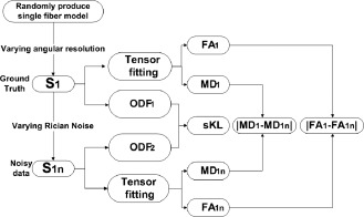
Flow chart for simulating diffusion signals from a single fiber. Different variations ( $\delta (\text{FA})\mathrm{=}\mathrm{|}{\text{FA}}_1\mathrm{-}{\text{FA}}_{1\mathrm{n}}\mathrm{|}$ and $\delta ({\text{MD}}_1)\mathrm{=}\mathrm{|}{\text{MD}}_1\mathrm{-}{\text{MD}}_{1\mathrm{n}}\mathrm{|}$) were used to evaluate the accuracy of tensor fitting in different simulations. sKL was used to evaluate the accuracy of ODF estimation for different simulations.

Tests combining real and simulated data

Even when the scan time is fixed, the relationships and optimal trade‐offs among SNR, spatial resolution, and angular resolution still depend, to some extent, on the subject being scanned and the diffusion profiles observed in a living brain. Thus, we designed the following tests to investigate these trade‐offs in real human brain datasets.

First, we investigated the effect of angular resolution, on its own, in real human brain data. We chose the highest angular resolution data with 48 directions (P1 in Table 1), to fit the diffusion tensor and calculate FA₄₈, MD₄₈, as well as estimate ODF₄₈. We then incrementally reduced the angular resolution from 48 to 47, 46, …, 6 directions that were recomputed to minimize the angular distribution energy. Our downsampling method, to do this, is detailed in Zhan et al. [2010b], and is designed to give a fair assessment of undersampled data by optimizing the angular distribution in the available data. For each angular resolution, we recalculated FA, MD and estimated the ODF. For the ODFs, the minimum number of angular samples was chosen to be 15 because that is the minimum number needed to fit 4th order SHs. To evaluate the angular sampling effect, cross‐correlation (Corr), and mutual information (MI) scalar maps were calculated to compare the original (P1) data to the down‐sampled data. Corr and MI are computed across all brain voxels in one subject and their arithmetic mean was computed across all subjects.

The MI between two images A and B is defined in Eq. (7).

$$\mathrm{I}(A,B)={\sum }_{a,b}p(a,b)·\log \frac{p(a,b)}{p(a)·p(b)}$$ (7)

MI measures the distance between the joint distribution of the images' intensity values p(a,b) and the joint distribution that would arise if the images were completely independent, p(a)p(b). MI is therefore a measure of dependence between two images. When MI is used to guide registration, the assumption is that there is maximal dependence between the intensity values of the images when they are correctly aligned, and misalignment will lead to a decrease in the MI. In this study, MI is built from the cumulative histogram of two images, where one is under‐sampled (i.e., fewer gradient directions) and the other is the full protocol. When making this histogram, data is pooled from all the voxels in the brain region. In addition, sKL was used to measure the ODF differences (estimation errors) between the original P1 data and each of the under‐sampled P1 datasets. This procedure allows us to investigate the amount of information lost by sacrificing angular resolution, while other parameters are fixed. In general, “better” approximations to the true DTI measures, are indicated by a higher Corr and MI between corresponding scalar maps (FA or MD), and smaller sKL distance between the ODFs in the original P1 and downsampled P1.

This angular downsampling will slightly overestimate the correlation achievable in scans of the same subject collected in independent scanning sessions, but by subsampling the same dataset, we can isolate the effect of angular sampling and model it in the absence of other sources of error. Figure 2 shows a flow chart indicating how we quantified the information loss when downsampling the angular resolution of the data.

Figure 2.

In this flow chart, we show how we used correlation and mutual information to assess how much information was lost when reducing the directional sampling of the DTI scans.

We next assessed the effect of spatial resolution by comparing datasets obtained with different voxel sizes, as outlined in Figure 3. We chose the highest spatial resolution data, with 2.5 mm isotropic voxels (P3 in Table 1), to calculate FA and MD. We then gradually reduced the spatial resolution by downsampling from (2.5 mm)³ to 2.6, 2.7, …(10 mm)³. Although other choices are possible, we used linear interpolation to downsample the spatial resolution of the original images in P3 to create each new image since P3 is the highest spatial resolution protocol in our study and the partial volume effect can be better modeled in compared with using the other two protocols. For each spatially downsampled dataset, we recalculated FA and MD. To evaluate the effect of reducing the spatial resolution, we again calculated Corr and MI between original and downsampled scalar maps for each subject and their arithmetic mean was computed across all brains.1 To do this, we upsampled the downsampled maps back to the original resolution and re‐calculated Corr and MI. This additional procedure was performed because as the spatial resolution changes, the number of voxels in the scan will also change accordingly. Therefore, to make the comparisons fair, all scalar maps were sampled on the same image matrix. This upsampling was performed using linear interpolation. We used the FA and MD calculated from the original P3 data as the ground truth since the original P3 data has the highest spatial resolution, and should contain the most spatial information. When downsampling, the spatial resolution will be lost—but the SNR should increase due to partial voluming effects. We firstly did not consider SNR varying due to spatial resolution changing. In this way, we examined voxel size effects while keeping the angular resolution constant.

Figure 3.

Flow chart for assessing how spatial resolution affects FA and MD, without allowing the SNR to confound the assessment. The ground truth is calculated from original P3 data with (2.5 mm)³ (indexed as 25), then downsample the spatial resolution to (2.6 mm)³ (indexed as 26), (2.7 mm)³ (indexed as 27), …, (10 mm)³ (indexed as 100).

Theoretically, the SNR is related to the voxel volume ( $\text{SNR}\mathrm{\propto }\text{volume}\mathrm{\times }\sqrt{\text{scanning}\hspace{1em}\text{time}}$), so changing the spatial resolution will affect the SNR. In a fixed scanning time, SNR is proportional to the voxel volume, so we used linear regression to relate SNR to the voxel volume based on the three protocols (P1, P2, and P3). The details are as follows.

T2‐weighted (b ₀) images for the P1, P2, and P3 datasets were aligned to the Colin27 high‐resolution single subject average brain MRI T1 template [Holmes et al., 1998] using the FLIRT linear registration software (http://fsl.fmrib.ox.ac.uk/fsl/flirt), with 9‐parameters (to account for translations, rotations, and scaling in each direction) and a mutual information cost function. Once linearly aligned, further registration was performed using a 3D Navier‐Stokes based fluid warping technique enforcing diffeomorphic mapping, using least‐squares intensity differences as a cost function [Leporé et al., 2009]. Deformation fields from the fluid registration steps were retained. Then a small spatially homogeneous region of interest (ROI, around 10 × 10 × 10 mm³) was manually traced on the corpus callosum (CC) in the Colin27 space using the “erosion with a 3D diamond” tool in the BrainSuite package [Shattuck and Leahy, 2002]. We then inverted the above transformation matrix and applied it to this ROI to create individual ROIs on the P1, P2, and P3 scans respectively, and SNR was computed as a ratio between the mean signal and its spatial standard deviation over the individual ROI in the original T2 (b ₀) images for each protocol [Zhan et al., 2010b]. We preferred this SNR estimation method since SNR is highly correlated with spatial resolution, so for each protocols in Table 1 , we need to estimate SNR in the individual space as fairly as possible. After we calculated the SNR for the three protocols, we used linear regression to model the relationship between SNR and voxel volume. Figure 4 shows the predicted SNR and the fitted line.

Figure 4.

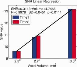
Linear least‐squares estimation for SNR vs. voxel volume. Here we show that there is a relative gain in SNR that is linear in the voxel volume; this SNR gain followed the equation shown on the plot. [Color figure can be viewed in the online issue, which is available at http://wileyonlinelibrary.com.]

After the SNR was related to voxel size, we continued to use P3 as a reference, it had the highest spatial resolution. We added Rician noise according to the SNR equation obtained from the linear least squares fit to create noisy P3 data, and calculated FA and MD. We then downsampled the original P3 data to give poorer spatial resolutions, added Rician noise accordingly, and calculated FA and MD. Finally, we upsampled all scalar maps back to the original image size and do the comparison (using Corr, MI). The flow chart of this part can be referred to Figure 3, the only difference is adding corresponding Rician noise when downsampling the spatial resolution.

Longitudinal stability

We also compared the temporal stability (test/retest reproducibility) of the three different protocols based on scans collected 2 weeks apart. All subjects' images (3 protocols and 2 time points) were linearly registered to the Colin27 space using the FLIRT algorithm using a 9‐parameter global registration and a mutual information cost function [Jenkinson and Smith, 2001; Jenkinson et al., 2002]. DTI‐derived scalar maps (FA, MD) and ODF were calculated from these registered data as before. Then the TDF framework was applied to analyze all these images, and the diffusion profile, P* [Eq. (3), Leow et al., 2009], was determined for each voxel in each brain (FSL's “bet” function was used to extract the brain) [Smith, 2002]. The exponential isotropy (EI) can be used to quantify the randomness of this probabilistic ensemble P*. The EI inversely measures how certainly (reliably) we can estimate the dominant fibers for each voxel. Thus, EI may be used to represent the information uncertainty; it has higher values in gray matter than white matter. EI can be calculated from Eq. (4). Then we evaluated longitudinal reproducibility for all scalar maps (DTI‐derived FA, MD, TDF‐derived EI) and the ODF across time for all three protocols. The longitudinal reproducibility (LR) at each voxel was computed from Eq. (8):

$$\text{LR}(\text{var})=\sum _{\mathrm{i}\mathrm{=}1}^N\frac{1}{N}\left|\frac{{\text{var}}_{\text{time}1}\mathrm{-}{\text{var}}_{\text{time}2}}{{\text{var}}_{\text{time}1}\mathrm{+}{\text{var}}_{\text{time}2}}\right|$$ (8)

Here var represents FA, MD and EI value for each voxel, and N is the number of subjects (8 in this study). The longitudinal reproducibility (LR) of the ODF field at each voxel was computed using the information‐theoretic distance, sKL, from Eq. (9):

$$\text{LR}(\text{ODF})=\sum _{\mathrm{i}\mathrm{=}1}^N\frac{1}{N}\mathrm{s}\mathrm{KL}(\text{ODF}{\mathrm{|}}_{\text{time}1}\mathrm{,}\text{ODF}\mathrm{|}{}_{\text{time}2})$$ (9)

Here sKL was calculated from Eq. (6), and N is the total number of subjects. The ODF values were sampled on a spherical surface at 642 points determined using a recursively subdivided icosahedral approximation of the unit sphere.

Tract‐based analysis

To assess how the choice of scanning protocol might affect a standard, widely‐used type of image analysis, we examined Tract‐Based Spatial Statistics (TBSS) using the TBSS toolbox in FSL [Smith et al., 2006]. We used the software on the human datasets (not the phantom) to assess the longitudinal reproducibility of FA along the fiber skeleton for protocols P1‐P3 from Table 1. As our eight subjects were all healthy adults, we aligned the two time point FA images from all subjects via nonlinear transformations to a target image, which was the FA image from ICBM young adult DTI‐81 atlas (http://www.loni.ucla.edu/ICBM/). The resulting data were then further affinely transformed into the 1x1x1 mm³ standard MNI152 space. From the registered FA maps, we computed mean FA skeletons. Then we defined 14 white matter ROIs along the mean FA skeleton (Table 2 , Column 1). We computed the longitudinal reproducibility of FA for each point in the skeleton based on Eq. 8. This allowed ROI‐based comparison of the protocols P1 − P3. For the phantom data, we used MedINRIA to extract one main fiber bundle using the Q‐ball tractography model and parameters of this tract were assessed for dependency on the protocol (P1 − P6 from Table 1 ).

Table 2.

Paired t‐test significance level comparing protocols for their longitudinal stability

ROIs	Comparisons
	P1<P2	P1<P3	P2<P1	P2<P3	P3<P1	P3<P2
Corpus Callosum	1	1	3.82E‐09	1	3.47E‐33	3.77E‐11
Cerebellar Peduncle	2.29E‐04	0.86	1	1	0.14	7.78E‐06
Cerebral Peduncle	0.01	0.44	0.99	0.99	0.56	0.01
Internal Capsule	1	1	4.69E‐03	0.97	1.66E‐06	0.03
Corona Radiata	2.63E‐37	1.43E‐06	1	1	1	4.18E‐16
Posterior Thalamic Radiation	1.47E‐08	1.69E‐05	1	0.93	1	0.07
Sagittal Stratum	0.98	1.20E‐03	0.02	1.92E‐07	1	1
External Capsule	0.99	1	0.01	1	7.85E‐09	8.00E‐04
Cingulum	0.91	1	0.09	1	6.24E‐17	8.05E‐12
Fornix and stria terminalis	0.01	4.87E‐11	0.99	1.00E‐04	1	1
Superior Longitudinal Fasciculus	3.90E‐07	0.84	1	1	0.16	2.81E‐08
Fronto‐Occipital Fasciculus	1.03E‐04	1.71E‐04	1	0.37	1	0.63
Uncinate Fasciculus	1.50E‐04	0.54	1	1	0.46	1.30E‐03
Tapetum	1.70E‐04	1.85E‐11	1	0.01	1	0.99

Here, the stability of the FA on the skeleton is assessed, in numerous ROIs used in TBSS analyses. As 6 contrasts were performed in 14 ROIs, the Bonferroni corrected significance level for these tests should be set to 0.05/(14 × 6), or 5.95 × 10⁻⁴. If a protocol outperforms the other two, at the Bonferroni threshold, it is underlined. See text for interpretation.

RESULTS AND DISCUSSION

SNR vs. Angular Resolution in Simulated Data

Figure 5 shows how the estimation error changes for the standard DTI‐derived scalar maps (FA, MD) and the HARDI‐derived ODF, (1) as the SNR increases, and (2) at different angular resolutions. Results differ when diffusion is modeled by a single tensor (Fig. 5a–c) or as two crossing tensors (Fig. 5d–f). At low SNR, increasing the angular resolution greatly improved the estimation accuracy both for the DTI‐derived scalars and for the ODF, but this mattered less when SNR was already high. Comparing Figure 5c and 5f, the sKL distance (i.e., the ODF reconstruction error) is smaller for the single‐ versus two‐tensor simulations, as poorly sampled data does a poorer job of capturing fiber crossings than single fibers. This is reasonable, as greater angular sampling is needed to estimate a more complex diffusion profile with the same accuracy when two tensors are present. Clearly, increasing the angular sampling improves estimation accuracy more when SNR is low, and when fiber crossing is present.

Figure 5.

This simulation shows that greater angular resolution improves the accuracy of estimating FA, MD, and the ODF, but only when the SNR is low. When only one tensor is present, the discrepancy between the ground truth and the approximated signal is less when the angular resolution is better (lower curves). (a–c) show this discrepancy, δ(MD), δ(FA), and sKL for the single‐tensor situation; (d–f) show δ(MD), δ(FA), and sKL, for the fibers that cross at 90°. The SNR level is chosen to vary from 5 to 50, and the angular resolution is varied from 10 to 100. Increasing the angular sampling improves estimation accuracy more when SNR is low, and when fiber crossing is present—in other words, the estimation accuracy is already relatively good in single‐fiber and high‐SNR situations. [Color figure can be viewed in the online issue, which is available at http://wileyonlinelibrary.com.]

Angular Resolution Effects in Real Data

Figure 6 shows how angular resolution affects DTI‐derived scalar maps. Figure 6a,b show MD and FA calculated from four different angular resolution subsets. Figure 6c,d show the correlation and mutual information between scalar maps calculated from the down‐sampled data and the original resolution data. As expected, more angular samples are needed for FA to converge to its true value, while MD converges to its true value more quickly, as the angular sampling is improved. The same pattern is seen for the MI (Fig. 6d). This suggests lower angular resolution is acceptable for computing MD relative to FA, which is consistent with our previous study of an independent HARDI dataset from young adults [Zhan et al., 2010b].

Figure 6.

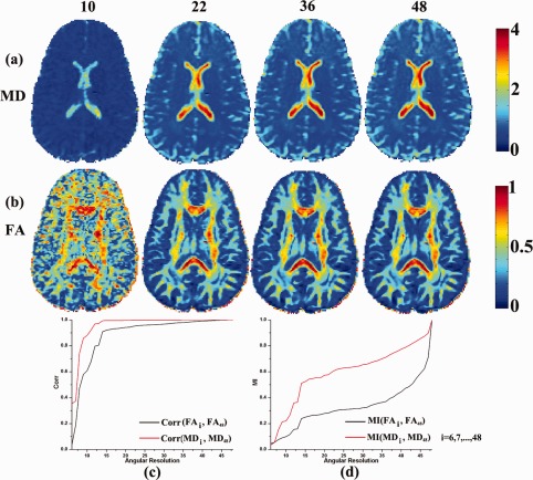
Angular resolution affects DTI‐derived scalar maps. At the top of the figure, we show the number of diffusion gradients (10, 22, 36, or 48) used to estimate the MD and FA maps, shown in rows (a) and (b). (c) Correlations are shown between between scalar maps derived from the highest angular resolution data versus the downsampled (lower angular resolution) data. As expected, the FA requires more angular samples to converge to its true value, while MD converges more quickly. (d) The MI value between scalar maps calculated from original angular resolution data and from downsampled angular resolution dataset. The MI curves are normalized to their maximum value. [Color figure can be viewed in the online issue, which is available at http://wileyonlinelibrary.com.]

Figure 7 shows how angular resolution affects the accuracy of ODF estimates. Figure 7a shows the ODF reconstructed from four different angular resolution subsets. Figure 7b shows the discrepancy (sKL) between ODFs reconstructed from the highest angular resolution data and the downsampled versions shown in Figure 7a. As expected, in Figure 7c, the discrepancy decreases as angular resolution increases, but with different patterns of improvement depending on the brain region. For the corpus callosum ROI, the sKL decreases more steadily compared to the sKL for ROIs with known fiber crossings in the superior longitudinal fasciculus (SLF) and corona radiata (Fig. 7c). This agrees with our simulation study in Section 3.1 (Figure 5c vs. 5f).

Figure 7.

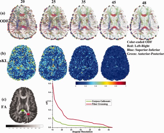
Greater angular sampling improves ODF reconstruction more when the ROI contains fiber crossings. The top row (a) shows ODF fields calculated from datasets with different angular resolutions; (b) shows the discrepancy (sKL) between the ODFs at the highest angular resolution versus ODFs from downsampled data with lower angular resolutions; (c,d) show sKL vs. angular resolution for two ROIs: the splenium of the corpus callosum (CC) and for fiber crossings in the SLF (superior longitudinal fasciculus), corona radiata, and corpus callosum. The ODF reconstruction error (sKL) for the CC is much smaller than in the fiber crossing region. In addition, the greater angular sampling offers greater improvement for reducing the ODF estimation error in the ROI where fibers cross. [Color figure can be viewed in the online issue, which is available at http://wileyonlinelibrary.com.]

Spatial Resolution Effects in Real Brain Data

Figure 8 shows how voxel size affects DTI‐derived scalar maps; here we do not consider the ODF, as its reconstruction in low spatial resolution data is complex. Figure 8a,b show FA and MD calculated at four different spatial resolutions, with and without artificially added noise. Figure 8c,f show plots of Corr and MI for FA and MD as the voxel sizes vary. Corr and MI decrease monotonically as the voxel sizes get bigger, from (2.5 mm)³ to (10 mm)³ (represented by the black curve in Figure 8c–f). As shown in the zoomed‐in insets, these effects are not monotonically decreasing—there is initially some evidence of a slightly better correlation as the voxel size increases, as the SNR is boosted by the bigger voxel size. Then the correlation falls rapidly, as the voxel size is too large to correctly resolve the details of the fiber geometry.

Figure 8.

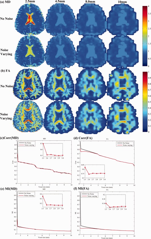
Errors in DTI‐derived scalar maps as the voxel size increases. Four increasing voxel sizes are shown (shown at the top, from left to right: 2.5, 4, 8, and 10 mm). For each, we computed MD (a) and FA (b) and compared their values with the measures computed at the highest resolution (2.5 mm). The correlations of the MD and FA from downsampled data versus the most accurate measure of MD (c) and FA (d) fall rapidly as the voxel size increases. This deteriorating correlation is found whether noise is artificially added (red curves) or not (black curves). Similar patterns are seen when MI is used to compare downsampled measures with the ground truth.

Longitudinal Stability

For many measures that we need to compute longitudinally (such as FA), it is not entirely clear if adding gradient directions is going to be better or worse in a fixed scan time, as the voxel size also has to be increased to keep the scan duration the same. When adding more directions under fixed scan duration, the voxels will eventually need to be so large that they would encompass multiple tracts and FA could not be reasonably obtained without severe partial voluming errors. Conversely, the use of larger voxels is not necessarily a bad thing, as it does boost the SNR for FA, which is also important for longitudinal consistency and reproducibility. However, it is not obvious what happens to the longitudinal stability of any of these measures as gradients are added and voxel sizes are varied to equalize scan times. Figure 9 compares the longitudinal stability of the three different protocols (described in Table 1), when our eight subjects were scanned twice over a short interval (2 weeks apart). Maps show the mean value of the stability, defined as abs( $\frac{\mathrm{time}\hspace{1em}1-\mathrm{time}\hspace{1em}2}{\mathrm{time}\hspace{1em}1+\mathrm{time}\hspace{1em}2}$) for the two DTI‐derived scalars (FA, MD) and the TDF‐derived EI, as well as the mean reconstruction error (sKL) for the derived ODF(time point1, time point2). The FA stability was notably poorer even with a relatively small reduction in the voxel size, from 2.7 to 2.5 mm. The EI, which uses the full set of gradients, was less dependent on the voxel size; such a measure may be useful in studies that have to combine data with different voxel sizes, such as meta‐analyses of studies that were designed independently. When voxels are larger, measures derived from DTI (MD, FA, sKL, and EI) were more reproducible over time, but partial volume averaging can cause incorrect reductions in the estimated FA, as well as other sources of biases and errors.

Figure 9.

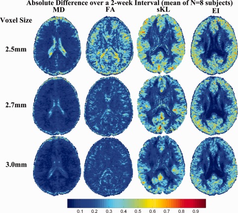
Longitudinal stability over a 2‐week interval. When voxels are larger, measures derived from DTI (MD, FA, sKL, and EI) are more reproducible over time. The more stable regions are shown in blue. Even so, the partial volume averaging can cause incorrect reductions in the estimated FA, and can lead to other biases and errors. [Color figure can be viewed in the online issue, which is available at http://wileyonlinelibrary.com.]

Clearly it would require enormous resources to study this problem in its full generality, with all scan durations being assessed. For ADNI specifically, the allotted time of 7 min was based on the feasibility of finishing a multimodal acquisition with several other scans in a 30‐min period (including standard anatomical data and FLAIR assessments for white matter lesions). Many other factors were also being traded off, such as the need to collect one versus two anatomical scans, or the relative need to collect a T2‐weighted scan to rule out or quantify vascular lesions. For the three protocols compared in this study, an upper limit (7 min) was imposed on the scan time and the rest of the parameters were optimized for a scan of this duration. It must be conceded that the exact trade‐off would differ if the available scan time were 10 rather than 7 min, or any other duration, leading to a new optimization problem to determine the optimum imaging parameters. Even so, the methodology of this article could be similarly applied to longer or shorter scans. Inevitably, some general conclusions would be the same as those of the current analysis: that larger voxels would help to conserve SNR, that FA SNR asymptotes slowly with the number of angular samples, and that the longitudinal stability of the protocols tends to be better when larger voxels are used. It is also important to know how the angular sampling affects the ODFs, which we examined here. The concepts and approach of this article are also more relevant when the available imaging time is quite short, making trade‐offs absolutely critical to evaluate. The trade‐offs matter less when a longer acquisition time is tolerable.

One limitation of our study is that we did not assess how coils with higher channel counts or even acceleration might impact the attainable results. Higher channel count coils, for example, have been shown to improve SNR. Higher spatial resolution, in particular, is very SNR demanding. If the phase‐encode matrix is held constant, then SNR scales as the voxel size, i.e., in proportion to the isotropic spatial resolution (in mm) to the third power. Since SNR only scales as the square‐root of acquisition time, higher channel count coils offer promise to improve spatial resolution while keeping the acquisition time reasonable [Ferré et al., 2012; Keil et al., 2011; Wiggins et al., 2009].

Another limitation of this study is that we did not consider a very broad range of spatial and directional resolutions, so the protocols that performed best here are not necessarily global optima for what could be achieved where state‐of‐the‐art technology is available. To avoid incurring enormous cost in this preparatory study, we had to estimate that the final ADNI DTI protocol was unlikely to have larger voxels than 3 mm, as few state‐of‐the‐art studies would have lower resolution. The choice of protocols was also based on experience showing that voxels much smaller than 2 mm tend to give relatively poor SNR, unless the scan time could be substantially increased, which would not be practical here. As such, we performed repeat scanning in the smallest sample of human subjects that we expected to give robust conclusions. We also scanned a specialized phantom using six protocols to broaden the range of protocols assessed. As we show such trade‐offs and variability in these protocols, a more detailed study with more time and resources available to scan subjects in 0.1 mm increments could be of great use to the general community; a more global optimum may be achievable, although it is not clear that it would substantially alter the findings here for multisite longitutinal analysis.

Tract‐Based Analysis

Figure 10 shows the skeleton of the mean FA map, overlaid on a single subject's FA map. These skeletons (and the FA map in each case) are derived using the different scanning protocols: P1, P2, and P3. There is no obvious visual difference among these images. Thus we calculated mean longitudinal reproducibility (LR) across all eight subjects for each protocol; we also ran pairwise t‐tests to assess any evidence that FA stability was better for any one protocol versus the others. In these tests, we examined measures defined on the skeleton of the mean FA map, in a set of ROIs. Table 2 shows the Student's paired t‐test significance level for 14 WM ROIs when comparing three protocols (P1–P3). The underlined in the table indicates which specific protocol (if any) has the best longitudinal stability in the ROIs defined on the skeleton. Future work is needed to compare protocols in terms of their accuracy for mapping fiber tract trajectories and connectivity matrices, so the best choice among these protocols in that context remains unknown.

Figure 10.

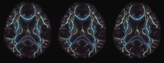
Mean FA skeleton overlaid on individual subject's FA for three protocols: P1, P2, and P3 (from left to right). There is no obvious visual difference for these TBSS measures; further analysis of longitudinal stability is in Table 2. [Color figure can be viewed in the online issue, which is available at http://wileyonlinelibrary.com.]

Interestingly, in Table 2, P3 (with the smallest voxels) gave best stability for the larger tracts, such as the corpus callosum and internal capsule, but P1 (with the most angular samples) gave greater stability for the more diffuse tracts that have a high degree of fiber crossing (corona radiata and long association fibers). Even so, there were exceptions to this general rule, and no protocol was a clear and consistent “winner” for longitudinal stability.

To pursue this question further, we investigated a broader range of protocols (P1‐P6 from Table 1) on the DTI phantom shown in Figure 11a (Pullens et al., 2010). An ROI was defined by hand to cover the whole fiber bundle (Fig. 11a,b) and MedINRIA was used, with a Q‐ball model, to reconstruct the fiber pathway. Figure 11(c–h) show the reconstructed fibers; parameters of these recovered fibers are summarized in Table 3.

Figure 11.

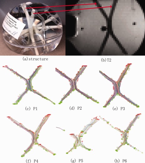
Fiber bundles were reconstructed from a specialized DTI phantom, scanned with various different protocols (P1–P6 from Table 1). (a) Photograph showing the phantom's structure; (b) Phantom T2 image; (c–h) fibers reconstructed with MedINRIA. The middle row shows scans with a standard b‐value (1,000 s/mm²) and the bottom row shows scans with a higher b‐value (3,000 s/mm²). In general, the high noise at higher b‐values makes it harder to reconstruct accurate fibers (P5, P6) but this can be mitigated by using more angular samples and larger voxels to boost SNR (P4). Overall, the traditional b‐value of 1,000 s/mm² gave most accurate reconstructions. [Color figure can be viewed in the online issue, which is available at http://wileyonlinelibrary.com.]

Table 3.

Fiber bundle parameters for different protocols

	P1	P2	P3	P4	P5	P6
Number of fibers	185	253	326	138	102	134
Min length (mm)	10.50	12.15	14.35	10.50	10.12	10.62
Max length (mm)	134.18	130.27	128.10	117.74	93.13	98.73
Mean length (mm)	78.88	95.55	92.09	69.04	38.78	51.31
Std length (mm)	34.80	30.54	31.92	28.18	15.22	25.27

See text for interpretation.

In Figure 11, the reconstructed fiber pathways were more accurate when derived from the protocols that used a standard b‐value (P1–P3); in general these gave intact fiber bundles. As seen in panels P5 and P6, it was more difficult to recover intact fibers from protocols with higher b‐values (from b = 3,000 s/mm²) unless the voxel size was higher, which serves to boost the SNR (P4). This is in line with intuition, because according to the Stejskal‐Tanner equation, $S_{\mathrm{q}}=S_0·\exp (-b·q^{\mathrm{T}}·D·q)$, a higher b‐value will lead to smaller measured diffusion signal S _q, which is more readily corrupted by noise [Zhan et al., 2009a], The better performance of P4 relative to the other high b‐value scans is consistent with prior studies showing that greater angular sampling can improve the SNR for diffusion measures [Zhan et al., 2009b, 2010b]. In Table 3, more fibers are extracted at a higher spatial resolution (P3), as the ODF tends to be sharper and less affected by partial voluming. Even so, the higher spatial resolution data are more corrupted by noise, and the mean fiber length is greatest for the intermediate protocol (P2 > P3 > P1). When the b‐value was standard (1,000), the largest voxels tended to limit the mean length of the paths, possibly due to partial voluming (which can make the fibers hard to track). But when the b‐value was increased, the data were more noisy overall, and the larger voxels ended up giving longer mean fiber length and a great number of fibers (see Table 3). As such, the best voxel size for tractography would appear to depend on the b‐value, with larger voxels being helpful to limit the effects of noise at high b‐values.

As shown in the bottom row of Figure 11, scans with higher b‐values tended to be noisier, when other factors were held constant. However, when angular resolution was highest (P4), the noise was mitigated to some extent; the higher b‐value protocol gave better reconstruction when the number of gradients was also high (P4). As a result, high b‐value scans should be reasonable to use, but due to their higher noise level, there is a tendency to need larger voxels to increase the SNR. If there is a need to resolve thinner tracts or more spatial detail, a reasonable trade‐off is to keep the diffusion weighting to more standard levels (such as 1,000 s/mm²) but allow smaller voxels. We note that the final 9‐min protocol used for ADNI was 2 min longer than originally planned, but the reason for the time increase was mainly to increase the FOV. This was found to be necessary to avoid occasional cropping of brain tissue that was happening at sites that began to use the 7‐min protocol.

In prior work, we also evaluated the benefits of using a higher b‐value—or even multiple b‐values at once, such as the 1,000, 2,000, and 3,000 s/mm² in our recent study using “staggered HYDI” or hybrid diffusion imaging [Zhan et al., 2011]. When comparing the spherical diffusion functions (orientation density functions or ODFs) recovered at different b‐values, we noticed that there was a higher uncertainty in estimating fiber eigenvalues but a more precise resolution of fiber directions as b‐values were increased. This is mainly due to the relative enhancement of diffusion along axonal fibers at higher b‐values, and relative suppression of random nonaxonal diffusion (see related work on CHARMED, by Assaf et al., 2005 and DSI, by Wedeen et al., 2005). It could be argued that the measurement of FA is more critical in AD biomarker studies than accurate recovery of tract directions, but clearly trade‐offs are involved and higher b‐values may be of interest in AD studies.

Involuntary Head Motion Evaluation

Prior studies have discussed how the physiological noise affects the DTI in population analysis [Walker et al., 2011]. Here we decided to confirm that head motion was comparable for the different protocols, to make sure that the protocol differences were not due to unmodeled differences in the amount of head motion. Motion in a time‐series of diffusion weighted images is typically estimated by retrospectively aligning all the diffusion gradient images to a nondiffusion‐sensitized baseline image. Clearly this may not recover all the motion, as the registration process has some error itself, but it is a fair estimate of the head motion present in the time‐series. We estimated the motion for each subject and protocol by affinely aligning each diffusion‐weighted image to a mean nondiffusion sensitized image (b ₀). We then defined the mean translation (MT) for the i‐th diffusion‐weighted image as ${\text{MT}}_i=\sqrt{(d_x^2+d_y^2+d_z^2)}$; then the MT for the whole dataset is defined as $\text{MT}=\frac{1}{N}{\Sigma }_{i=1}^N{\mathrm{MT}}_i$, in which i = 1,2,…,N and N is the total number of diffusion‐weighted images. We found the mean MT across the eight subjects in our study and two time points; values were 2.80 mm, 2.31 mm, and 2.04 mm for the three protocols (P1, P2, and P3). Paired two‐tailed t tests between P1 and P2, P1, and P3 and P2 and P3 motion levels detected no protocol‐related differences in the average amount of head motion at the 5% significance level (P = 0.34, 0.08, and 0.19 respectively). This is reasonable, as all scans took the same amount of time. Even so, we acknowledge that motion levels may affect the computed value of FA, even after motion correction (tending to reduce FA if motion is random and isotropic).

CONCLUSIONS

Clearly, if a major goal of a DTI study is to measure FA and compare it across subjects, it may be more important to minimize the error in estimating the diffusion eigenvalues than the error in estimating their dominant directions, although both are clearly important. Many studies now use voxel‐based methods to compare FA across groups, using methods such as “tract based spatial statistics” [TBSS: Smith et al., 2006] or whole‐brain statistical parametric maps [Braskie et al., 2011; Jahanshad et al., 2012b]. For ADNI, we expected FA maps, and regional summaries of FA, to be a key target of analysis as they show robust differences between groups of MCI and AD patients and matched controls. In the future however, tractography and even network‐based measures of fiber connectivity [Nir et al., 2012] may show promise for diagnosis and for predicting future brain and cognitive changes as we age. It must be conceded that these acquisition protocols are not optimized for tractography‐based connectivity studies, but are more suited for TBSS type voxelwise analyses.

Our study had three main conclusions. First, in the three scanning protocols with fixed scan time (7 min), scans with larger voxels gave better longitudinal stability (Fig. 9) and higher SNR (Fig. 4). In line with theoretical predictions, we verified empirically that the SNR went up by about 50% as the voxel size went up from 2.5 mm to 3mm, and the relationship between SNR and voxel volume was linear. This is worth considering practically, as there is a common tendency to favor scans with smaller voxels, but this may not be optimal when scan times limit the available SNR. Even so, errors in the derived measures increase as more tissues of different kinds (e.g., GM and WM), and more fibers with different dominant directions are included in the same voxel. The underestimation of FA, in particular, can be addressed to some extent by using a “beyond‐tensor” model of diffusion, such as the tensor distribution function model used to compute ODFs; the same model may be used to compute an adjusted measure of FA [Leow et al., 2009, Zhan et al., 2009a, 2010c].

Second, we performed simulations to separately assess the effects of angular and spatial resolution, which were correlated in the scans we collected as one was deliberately reduced to improve the other. In these simulations, better angular sampling helped to resolve the details of the diffusion geometry—but this effect was most evident when (1) SNR was low, and (2) more than one fiber per voxel was present. In Figure 5, our calibration curves show that show the angular sampling suppresses reconstruction errors in the ODF, even well beyond the number of gradients that would typically suffice to estimate FA and MD (with further improvements with >100 gradients).

Our third conclusion was that around 20–30 diffusion gradients were helpful for resolving fiber crossing geometries (Fig. 7). There were also greater ODF estimation errors when using 2.5 mm versus 3.0 mm voxels.

This study has strengths and limitations. Among its strengths are the scanning of multiple subjects (8), each with several protocols and repeated scans, allowing assessments of longitudinal reproducibility. As the effects of angular and spatial resolution were traded off and were confounded in the real data, we also showed simulations and artificially resampled real data to separate the effects of voxel size and angular sampling. Among the limitations of the study are that we did not compare the protocols for mapping fiber tract trajectories and connectivity matrices. Although we plan such a study, it was not as immediate a goal as assessing the temporal stability of the most commonly derived diffusion indices, FA, MD, and the HARDI‐type measures such as the ODF.

The true value of DTI scanning, and the protocol used to collect it, is really only clear when the statistical outcomes of the study are known. This may include localizing brain regions or connections that differ between patients and controls, or discriminating people with MCI who will imminently develop AD. As the statistical power of the study depends on the question asked and the image analysis too, it is not possible to infer that the best DTI protocol in terms of SNR and reproducibility will be the one that gives most powerful results for discriminating disease. In addition, some SNR differences can arise from the variation in the TR, but this effect is expected to be small as the TRs are all relatively long compared with the T1 of WM and GM.

In reality, the final protocol selected for the diffusion imaging portion of ADNI was the 2.7‐mm protocol, as it offered a reasonable trade‐off among the benefits of large voxels (higher SNR and longitudinal stability), reasonable angular detail for ODF reconstruction, and acceptable spatial detail for reducing the partial volume effect. A further modification was made, after this study was performed, to increase the field‐of‐view, as the pilot protocols had led to cropping of brain tissue at several sites. This led to a DTI protocol lasting around 9 min, which is still feasible for a clinical study. Financial factors were also relevant as longer scans may cost more to collect, depending on how scanner time is billed.

Depending on the goals of the particular study, a more advanced HARDI protocol or longer scan may be feasible, but this study offers some practical guidelines for people developing diffusion protocols for clinical populations.

REFERENCES

- Aganj I, Lenglet C, Sapiro G, Yacoub E, Ugurbil K, Harel N (2010): Reconstruction of the orientation distribution function in single and multiple shell q‐ball imaging within constant solid angle. Magn Reson Med 64:554–566. [DOI] [PMC free article] [PubMed] [Google Scholar]
- Assaf Y, Basser PJ (2005): Composite hindered and restricted model of diffusion (CHARMED) MR imaging of the human brain. NeuroImage 27:48–58. [DOI] [PubMed] [Google Scholar]
- Braskie MN, Jahanshad N, Stein JL, Barysheva M, McMahon KL, de Zubicaray GI, Martin NG, Wright MJ, Ringman JM, Toga AW, Thompson PM (2011): Common Alzheimer's disease risk variant within the CLU gene affects white matter microstructure in young adults. J Neurosci 31:6764–6770. [DOI] [PMC free article] [PubMed] [Google Scholar]
- Chiang MC, McMahon KL, de Zubicaray GI, Martin NG,Hickie I, Toga AW, Wright MJ,Thompson PM (2010): Genetics of White Matter Development: A DTI Study of 705 Twins and Their Siblings Aged 12 to 29 (in press). [DOI] [PMC free article] [PubMed]
- Descoteaux M, Angelino E, Fitzgibbons S, Deriche R (2007): Regularized fast and robust analytical Q‐ball imaging. Magn Reson Med 58:497–510. [DOI] [PubMed] [Google Scholar]
- Ferré JC, Petr J, Bannier E, Barillot C, Gauvrit JY (2012): Improving quality of arterial spin labeling MR imaging at 3 Tesla with a 32‐channel coil and parallel imaging. J Magn Reson Imaging 2012. doi: 10.1002/jmri.23586. [Epub ahead of print] [DOI] [PubMed] [Google Scholar]
- Funk P (1916): Uber eine geometrische Anwendung der Abelschen Integralgleichung. Mathematische Annalen 77:129–135. [Google Scholar]
- Holmes CJ, Hoge R, Collins L, Woods R, Toga AW, Evans AC (1998): Enhancement of MR images using registration for signal averaging. J Comput Assist Tomography 22:324–333. [DOI] [PubMed] [Google Scholar]
- Jahanshad N, Zhan L, Bernstein MA, Borowski B, Jack CR, Toga AW, Thompson PM (2010): Diffusion tensor imaging in seven minutes: Determining trade‐offs between spatial and directional resolution, ISBI 2010, Rotterdam, the Netherlands.
- Jahanshad N, Zhan L, Bernstein MA, Borowski BJ, Jack CRJr, Toga AW, Thompson PM (2012a): Trade‐offs between directional and spatial resolution in diffusion tensor imaging within clinical time constraints, submitted to NeuroImage.
- Jahanshad N, Aganj I, Lenglet C, Jin Y, Joshi A, Barysheva M, McMahon KL, de Zubicaray GI, Martin NG, Wright MJ, Toga AW, Sapiro G, Thompson PM (2011): High angular resolution diffusion imaging (HARDI) tractography in 234 young adults reveals greater frontal lobe connectivity in women, ISBI2011.
- Jahanshad N, Kohannim O, Hibar DP, Stein JL, McMahon KL, de Zubicaray GI, Medland SE, Montgomery GW, Whitfield JB, Martin NG, Wright MJ, Toga AW, Thompson PM (2012b): Brain structure in healthy adults is related to serum transferrin and the H63D polymorphism in the HFE gene. Proc Natl Acad Sci USA: doi: 10.1073/pnas.1105543109. January 9, 2012. [DOI] [PMC free article] [PubMed] [Google Scholar]
- Jenkinson M, Smith S (2001): A global optimisation method for robust affine registration of brain images. Med Image Anal 5:143–156. [DOI] [PubMed] [Google Scholar]
- Jenkinson M, Bannister P, Brady J, Smith S (2002): Improved optimisation for the robust and accurate linear registration and motion correction of brain images. NeuroImage 17:825–841. [DOI] [PubMed] [Google Scholar]
- Jian B, Vemuri BC, Ozarslan E, Carney PR, Mareci TH (2007): A novel tensor distribution model for the diffusion‐weighted MR signal. NeuroImage 37:164–176. [DOI] [PMC free article] [PubMed] [Google Scholar]
- Jones DK, Horsfield MA, Simmons A (1999): Optimal strategies for measuring diffusion in anisotropic systems by magnetic resonance imaging. Magn Reson Med 42:515–525. [PubMed] [Google Scholar]
- Jones DK (2004): The effect of gradient sampling schemes on measures derived from diffusion tensor MRI: A Monte Carlo study. Magn Reson Med 51:807–815. [DOI] [PubMed] [Google Scholar]
- Keil B, Alagappan V, Mareyam A, McNab JA, Fujimoto K, Tountcheva V, Triantafyllou C, Dilks DD, Kanwisher N, Lin W, Grant PE, Wald LL (2011): Size‐optimized 32‐channel brain arrays for 3 T pediatric imaging. Magn Reson Med 66:1777–1787. [DOI] [PMC free article] [PubMed] [Google Scholar]
- Landman BA, Farrell JAD, Smith SA, Mori S, Prince JL (2007): Tradeoffs between tensor orientation and anisotropy in DTI: Impact of Diffusion Weighting Scheme. Proc ISMRM, 15th Scientific Meeting, Berlin.
- Le Bihan D (1990a): IVIM method measures diffusion and perfusion. Diagn Imaging (San Franc) 12:133–136. [PubMed] [Google Scholar]
- Le Bihan D (1990b): Magnetic resonance imaging of perfusion. Magn Reson Med 14:283–292. [DOI] [PubMed] [Google Scholar]
- Leow AD, Zhu S, Zhan L, McMahon K, de Zubicaray GI, Meredith M, Wright MJ, Toga AW, Thompson PM (2009): The tensor distribution function. Magn Reson Med 61:205–214. [DOI] [PMC free article] [PubMed] [Google Scholar]
- Lepore N, Chou YY, Lopez OL, Aizenstein HJ, Becker JT, Toga AW, Thompson PM (2008): Fast 3D Fluid Registration of Brain Magnetic Resonance Images, SPIE 2008. [DOI] [PMC free article] [PubMed]
- Lepore N, Brun CC, Descoteaux M, Lee AD, Barysheva M, Chou YY, McMahon KL, de Zubicaray GI, Martin NG, Wright MJ, Gee JC, Thompson PM (2010): A Multivariate Groupwise Genetic Analysis of White Matter Integrity using Orientation Distribution Functions, MICCAI Workshop on Computational Diffusion MRI, Beijing, China, 20–24 September 2010.
- Liu XX, Zhu T, Gu TL, Zhong JH (2010): Optimization of in vivo high‐resolution DTI of non‐human primates on a 3T human scanner. Methods 50:205–213. [DOI] [PubMed] [Google Scholar]
- Nir T, Jahanshad N, Jack CR, Weiner MW, Toga AW, Thompson PM; and the Alzheimer's Disease Neuroimaging Initiative (ADNI) (2012): Small world network measures predict white matter degeneration in patients with early‐stage mild cognitive impairment. ISBI2012, in press. [DOI] [PMC free article] [PubMed]
- Pennec X, Fillard P, Ayache N (2004): A Riemannian framework for tensor computing. Int J Comput Vis 66:41–66. [Google Scholar]
- Pullens P, Roebroeck A, Goebel R (2010): Ground truth hardware phantoms for validation of diffusion‐weighted MRI applications. J Magn Reson Imaging 32:482–488. [DOI] [PubMed] [Google Scholar]
- Shannon CE (1948): A mathematical theory of communication. Bell Syst Tech J 27:623–656. [Google Scholar]
- Shattuck DW, Leahy RM (2002): BrainSuite: An automated cortical surface identification tool. Med Image Anal 6:129–142. [DOI] [PubMed] [Google Scholar]
- Smith SM (2002): Fast robust automated brain extraction. Hum Brain Mapp 17:143–155. [DOI] [PMC free article] [PubMed] [Google Scholar]
- Smith SM, Jenkinson M, Johansen‐Berg H, Rueckert D, Nichols TE, Mackay CE, Watkins KE, Ciccarelli O, Cader MZ, Matthews PM, Behrens TEJ (2006): Tract‐based spatial statistics: Voxelwise analysis of multi‐subject diffusion data. NeuroImage 31:1487–1505. [DOI] [PubMed] [Google Scholar]
- Sporns O (2010):Networks of the Brain.Cambridge MA:MIT Press. [Google Scholar]
- Stejskal EO, Tanner JE (1965): Spin diffusion measurements: Spin echoes in the presence of a time‐dependent field gradient. J Chem Phys 42:288–292. [Google Scholar]
- Tuch DS, Weisskoff RM, Belliveau JW, Wedeen VJ (1999): High angular resolution diffusion imaging of the human brain. Proceedings of the 7th Annual Meeting of the ISMRM, Philadelphia.
- Tuch DS, Reese TG, Wiegell MR, Makris N, Belliveau JW, Wedeen VJ (2002): High angular resolution diffusion imaging reveals intravoxel white matter fiber heterogeneity. Magn Reson Med 48:577–582. [DOI] [PubMed] [Google Scholar]
- Tuch DS (2004): Q‐ball Imaging. MRM 52:1358–1372. [DOI] [PubMed] [Google Scholar]
- Wagner M, Fuchs M (2001): Integration of Functional MRI, Structural MRI, EEG, and MEG. Int J Bioelectromagn 3:1. [Google Scholar]
- Walker L, Chang LC, Koay CG, Sharma N, Cohen L, Verma R, Pierpaoli C (2011): Effects of physiological noise in population analysis of diffusion tensor MRI data. Neuroimage 54:1168–1177. [DOI] [PMC free article] [PubMed] [Google Scholar]
- Wedeen VJ, Hagmann P, Tseng WY, Reese TG, Weisskoff RM (2005): Mapping complex tissue architecture with diffusion spectrum magnetic resonance imaging. MRM 54:1377–1386. [DOI] [PubMed] [Google Scholar]
- Wiggins GC, Polimeni JR, Potthast A, Schmitt M, Alagappan V, Wald LL (2009): 96‐Channel receive‐only head coil for 3 Tesla: Design optimization and evaluation. Magn Reson Med 62:754–762. [DOI] [PMC free article] [PubMed] [Google Scholar]
- Wong STS, Roos MS (1994): A strategy for sampling on a sphere applied to 3D selective RF pulse design. Magn Reson Med 32:778–784. [DOI] [PubMed] [Google Scholar]
- Zhan L, Leow AD, Barysheva M, Feng A, Toga AW, Sapiro G, Harel N, Lim KO, Lenglet C, McMahon KL, de Zubicaray GI, Wright MJ, Thompson PM (2009a): Investigating the uncertainty in multi‐fiber estimation in high angular resolution diffusion imaging, MICCAI2009 Workshop on Probabilistic Modeling in Medical Image Analysis (PMMIA).
- Zhan L, Leow AD, Zhu S, Chiang MC, Barysheva M, Toga AW, McMahon KL, de Zubicaray GI, Wright MJ, Thompson PM (2009b): Analyzing multi‐fiber reconstruction in high angular resolution diffusion imaging using the tensor distribution function, Imaging Science and Biomedical Imaging (ISBI2009), Boston, MA.
- Zhan L, Leow AD, Jahanshad N, Lee AD, Barysheva M, Toga AW, McMahon KL, de Zubicaray GI, Martin NG, Wright WJ, Thompson PM (2010a): Genetic Analysis of High Angular Resolution Diffusion Images (HARDI), MICCAI Workshop on Computational Diffusion MRI, Beijing, China, 20–24 September 2010.
- Zhan L, Leow AD, Jahanshad N, Chiang MC, Barysheva M, Lee AD, Toga AW, McMahon KL, de Zubicaray GI, Wright MJ, Thompson PM (2010b): How does angular resolution affect diffusion imaging measures? Neuroimage 49:1357–1371. [DOI] [PMC free article] [PubMed] [Google Scholar]
- Zhan L, Leow AD, Jahanshad N, Toga AW, Thompson PM (2010c): Fiber Demixing with the Tensor Distribution Function avoids errors in Fractional Anisotropy maps, Organization for Human Brain Mapping, Barcelona, Barcelona, Spain.
- Zhan L, Leow AD, Aganj I, Lenglet C, Sapiro G, Yacoub E, Harel N, Toga AW, Thompson PM (2011): Differential information content in staggered multiple shell HARDI measured by the tensor distribution function, ISBI2011.