Integrating Chemical Footprinting Data into RNA Secondary Structure Prediction

Abstract

Chemical and enzymatic footprinting experiments, such as shape (selective 2′-hydroxyl acylation analyzed by primer extension), yield important information about RNA secondary structure. Indeed, since the -hydroxyl is reactive at flexible (loop) regions, but unreactive at base-paired regions, shape yields quantitative data about which RNA nucleotides are base-paired. Recently, low error rates in secondary structure prediction have been reported for three RNAs of moderate size, by including base stacking pseudo-energy terms derived from shape data into the computation of minimum free energy secondary structure. Here, we describe a novel method, RNAsc (RNA soft constraints), which includes pseudo-energy terms for each nucleotide position, rather than only for base stacking positions. We prove that RNAsc is self-consistent, in the sense that the nucleotide-specific probabilities of being unpaired in the low energy Boltzmann ensemble always become more closely correlated with the input shape data after application of RNAsc. From this mathematical perspective, the secondary structure predicted by RNAsc should be ‘correct’, in as much as the shape data is ‘correct’. We benchmark RNAsc against the previously mentioned method for eight RNAs, for which both shape data and native structures are known, to find the same accuracy in 7 out of 8 cases, and an improvement of 25% in one case. Furthermore, we present what appears to be the first direct comparison of shape data and in-line probing data, by comparing yeast asp-tRNA shape data from the literature with data from in-line probing experiments we have recently performed. With respect to several criteria, we find that shape data appear to be more robust than in-line probing data, at least in the case of asp-tRNA.

Introduction

RNA is an important biomolecule, known to play both an information carrying and a catalytic role. RNA plays roles in numerous biological processes, including retranslation of the genetic code (selenocysteine insertion, ribosomal frameshift), transcriptional and translational gene regulation, temperature-dependent allosteric regulation, chemical modification of specific nucleotides in the ribosome, regulation of alternative splicing, apparent regulation of the formation of heterochromatin, etc. (See [1] for a recent review on the analysis of sequence and structure of such noncoding RNA.) Since the function of non-coding RNA largely depends on its structure and since it is believed that RNA plays many yet undiscovered roles in cellular processes, it is important to determine the structure of RNA.

A secondary structure for a given RNA nucleotide sequence is a set of base pairs , such that forms either a Watson-Crick or GU (wobble) base pair, and such that there are no base triples or pseudoknots in . In this context, a base triple in consists of two base pairs , or , . A pseudoknot in consists of two base pairs , with . Although it is NP-hard [2] to compute the minimum free energy (MFE) tertiary (or even pseudoknotted) structure of RNA [3], the MFE secondary structure can be computed in time that is cubic in the input sequence length [4]. Moreover, it is widely believed that RNA folds in a hierarchical fashion [5]–[8], with the secondary structure acting as a scaffold for tertiary structure, although this is not universally accepted [9].

RNA secondary structure can be predicted by Zuker and Stiegler's algorithm [4], implemented in mfold [10], RNAfold [11], and RNAstructure [12]. This algorithm uses dynamic programming with free energy parameters from the Turner energy model [13] to compute the minimum free energy (MFE) structure.

A first step towards integrating chemical/enzymatic probing data was taken by Mathews et al. [14], where Zuker and Stiegler's algorithm was modified to support hard constraints reflecting the experimental data. In particular, given an RNA sequence, the software RNAstructure [14] computed the minimum free energy (MFE) secondary structure subject to user-defined constraints, such as stipulating that particular nucleotides remain unpaired, that pairs of specific nucleotides form a base pair, etc. Mathews et al. reported that the MFE structure prediction with (hard) constraints corresponding to chemical modification (1-cyclohexyl-3-(2-morpholinoethyl) carbodiimide metho-p-toluene sulfonate, dimethyl sulfate, and kethoxal) yielded an improvement in base-pair accuracy for 5S rRNA of E. coli from 26.3% to 86.8% [14]. (See [15] for more remarks and a less optimistic evaluation of RNAstructure with hard constraints on 16S rRNA.)

Chemical/enzymatic probing data is probabilistic in nature, as exemplified in pars footprinting data [16]. Rarely is it absolutely clear that certain positions are unpaired, or that certain base pairs are formed; instead, there is a certain probability of these events. In moving away from error-prone hard constraints, Deigan et al. [15] took a second step of incorporating shape (selective -hydroxyl acylation analyzed by primer extension) data [17], [18], whose numerical values (continuously) range from 0 to approximately 2.2, by incorporating a pseudo free energy for base stacking into the Zuker algorithm. The pseudo free energy term in [15] was defined to be

(1)

where kcal/mol and kcal/mol, for each position occurring in a base pairing stack; if is unpaired, then no pseudo free energy is added. (The position is in a base pairing stack if 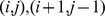are base pairs, or if are base pairs belonging to the secondary structure. For base pairs that are surrounded by base pair neighbors and , the pseudo-energy term is applied twice.) The resulting modified version of Zuker and Stiegler's algorithm, as implemented in RNAstructure was reported to yield secondary structure prediction accuracies of up to for three moderate-sized RNAs ( nt) and for 16S rRNA ( nt). Wilkinson et al. [19] later described a model for the secondary structure of the HIV-1 genome, as computed by RNAstructure with shape pseudo energies defined in equation 1. If correct, this is a remarkable feat, given that the size of the HIV-1 genome is generally just under 10,000 nt (see http://www.hiv.lanl.gov), hence several times larger than the ribosome, whose crystal structure was only determined after years of painstaking work (the large unit, PDB code 1FFK [20], of the ribosome of Haloarcula marismortui consists of a 23S chain of length 2,922 nt and a 5S chain of 122 nt).

One issue with this approach is that it takes into consideration shape data only for base-stacked positions, i.e., a pseudo free energy term corresponding to shape data is applied at positions where a stacked base pair occurs, but not where nucleotides are unpaired. By ignoring shape data for unpaired nucleotide positions, this approach can thus bias structure prediction to form base pairs even at positions, which shape data may suggest are flexible. Indeed the expected distance of predicted base pairing probabilities computed by RNAstructure with shape values increases after the incorporation of the shape pseudo energy terms (see Table 1). (As later defined, RNAstructure and RNAsc both compute the probability that base pair belongs to a structure in the low energy Boltzmann ensemble. Since the pseudo energy model for shape data incorporation is different in RNAstructure and RNAsc, the base pairing probabilities and Boltzmann low energy ensembles may be different.) In contrast to the pseudo energies of RNAstructure, our algorithm RNAsc, will always shift the distribution of conformations towards the shape measurements (see Methods for a mathematical proof).

Table 1. Benchmark results.

Secondary structure prediction accuracy
RNA	len	test	(A)	(B)	(C)	RNA	len	test	(A)	(B)	(C)
asp-tRNA	75	sens.	1.00	1.00	0.76	phe-tRNA	76	sens.	1.00	0.75	0.95
		ppv	1.00	1.00	0.76			ppv	0.95	0.71	0.95
		ave ent.	0.21	0.17	0.27			ave ent.	0.2	0.17	0.46
		str. div.	19.53	17.17	22.60			str. div.	11.37	9.38	34.37
		edist.	23.7	61.77	24.9			edist.	29.51	61.77	33.68
HCV IRES	95	sens.	0.96	0.96	0.96	5S rRNA	120	sens.	0.94	0.94	0.26
		ppv	1.00	1.00	1.00			ppv	0.82	0.82	0.22
		ave ent.	0.05	0.06	0.27			ave ent.	0.30	0.17	0.27
		str. div.	3.20	3.57	21.45			str. div.	46.93	20.70	32.90
		edist.	31.36	52.48	36.53			edist.	42.57	54.01	46.41
P546	155	sens.	0.95	0.96	0.43	glycine	162	sens.	0.92	0.92	0.70
		ppv	0.96	0.98	0.44			ppv	0.84	0.84	0.61
		ave ent.	0.18	0.12	0.38			ave ent.	0.11	0.05	0.30
		str. div.	27.7	14.05	66.50			str. div.	15.14	5.13	44.16
		edist.	41.36	131.77	56.11			edist.	53.90	115.55	60.29

A comparison of three secondary structure prediction algorithms, using shape data from Deigan et al. [15] for the three RNA molecules, yeast aspartyl tRNA (asp-tRNA), hepatitis C virus internal ribosomal entry site (HCV IRES), and the P546 domain from the bI3 group I intron (P546), along with shape data from [26] for three additional RNA molecules, E. coli phenylalanine tRNA (phe-tRNA), E. coli 5S ribosomal RNA (5S rRNA), and F. nucleatum glycine riboswitch (glycine). The benchmark results are tabulated for (A) RNAsc+shape, (B) RNAstructure+shape, and (C) RNAstructure (with no shape data). Sensitivity is abbreviated by sens., positive predictive value is abbreviated by ppv. The average pointwise entropy, Morgan-Higgs structural diversity, and the expected distance of the computed probabilities to the probing data are abreviated by ave ent., str. div., and edist., respectively. Not shown: results for medloop and V. vulnificus adenine riboswitch (1Y26), for which all three methods have optima sensitivity and ppv values of 1.0.

Nonetheless, MFE dynamic programming methods that incorporate high throughput chemical/enzymatic footprinting data can yield important insights into the structure and function of RNA molecules, much faster than the labor-intensive X-ray diffraction methods.

The motivation for our work is to develop a method that incorporates chemical/enzymatic footprinting data in a self-consistent manner. In particular, given experimental data of the form , where is the experimental probability that the th nucleotide is unpaired (or, more accurately, in a flexible region, as witnessed by high shape reactivity), our goal is to develop an algorithm incorporating footprinting data such that the recalculated probabilities are guaranteed to be closer to the experimental measurements. If our algorithm is self-consistent in this manner, then we have strong mathematical evidence that the partition function computation and hence the MFE computation are both as correct as is the shape data. In contrast to the pseudo energies of RNAstructure, we prove that our algorithm RNAsc is self-consistent, and on average, the ensemble of low energy secondary structures produced by our method yields a footprinting pattern that closely resembles the pattern from input experimental shape data. We benchmark our method against the RNAstructure program [19] on eight RNAs, for which shape data and native structures are both available. The secondary structure predictions from our method and from RNAstructure are fairly similar and both significantly improve secondary structure prediction without incorporation of footprinting data (e.g. mfold, RNAfold). However, the expected distance of the computed probabilities with the shape data is lower in our method for all the test cases. It is worth noting that the mistakes in the predicted secondary structure usually occur in positions where the shape data might be inaccurate, or where the native structure and shape data structures could be somewhat different, due to quite different temperatures required by each experimental protocol. Recent studies have shown that different experimental mapping approaches can provide complementary structural information [21]. Thus, we additionally performed in-line probing [22], [23] on asp-tRNA, in order to compare the results of shape and in-line probing in the context of our algorithm. The source code of RNAsc as well as a web server is available at http://bioinformatics.bc.edu/clotelab/RNAsc/.

Methods

In-line probing experiments

DNA oligonucleotides for the sequence and its reverse complement were purchased from MWG Operon; remaining reagents were obtained from Sigma-Aldrich. DNA oligonucleotides were annealed to create templates for T7 polymerase transcription, and the transcription products were purified by denaturing PAGE and eluted in 10 mM Tris-HCl (pH 7.5 at C), 200 mM NaCl and 1 mM EDTA. Following in-line probing protocols designed by the Breaker Lab [22], [23], synthesized RNA molecules were dephosphorylated using alkaline phosphatase (Roche Diagnostics) and radiolabeled with [g-32P]ATP and T4 polynucleotide kinase (NEB) according to the manufacturers instructions. Spontaneous transesterification reactions using PAGE-purified, endlabeled RNAs were assembled as described in [23]. Incubations were performed for approximately 40 h at C in 10-uL volumes containing 50 mM Tris-HCl (pH 8.3 at C), 20 mM MgCl2, 100 mM KCl and nM RNA. RNA fragments resulting from spontaneous transesterification were resolved by denaturing 10% PAGE, and imaged with a Molecular Dynamics STORM PhosphorImager. Quantification of gels were performed using SAFA (Semi-Automated Footprinting Analysis) [24]. In-line probing experiments were repeated an additional two times, resulting in gels with comparable data (data not shown). Fig. 1 is an image of the in-line probing gel for yeast asp-tRNA.

Figure 1. In-line probing.

Spontaneous cleavage pattern resulting from in-line probing of yeast asp-tRNA, nucleotides with larger backbone flexibility will have higher rates of cleavage and thus bands of greater intensity. Lanes for no reaction, T1 RNase (cleavage following only guanosines), and partial hydroxyl cleavage (-OH, cleavage after each base) are indicated. Due to the high resolution of the gel, double bands appear for nucleotides 2–9. These bands correspond to RNA molecules where the cyclic phosphate intermediate has hydrolyzed to leave either no phosphate, or a mixture of - and -phosphate products which migrate more quickly on the gel. Quantifcation of these positions combined the bands corresponding to both products. The precursor RNA and T1 RNase cleavage products are marked. Not all guanosines show cleavage due to retention of secondary structure at 5 M urea and elevated temperature.

Computational methods

Briefly stated, our algorithm, RNAsc (RNA soft constraints), consists of a preprocessing step, that normalizes shape data to the range , followed by a computation of the minimum free energy [resp. partition function], which incorporates pseudo-energy terms [resp. Boltzmann factors of pseudo-energy terms] for each nucleotide position. We begin by discussion of the normalization of shape data.

Normalization of shape

In experiments reported by the Weeks Lab [25] as well as the Das Lab [26], shape reactivities range from to roughly . Large reactivities suggest that the position is unpaired; small reactivities suggest that the position is base-paired. More specifically, nucleotides with shape reactivities or are considered highly and moderately reactive, respectively [15]. The normalization is carried out in a piecewise linear fashion where will be roughly mapped to . However, very low shape reactivities should not be mapped close to either as it will bias the shape values toward unpaired nucleotides. For this reason the shape reactivity values are linearly mapped to the interval , the reactivity values in are linearly mapped to the interval , the reactivity values in are linearly mapped to the interval , and lastly, the reactivities are linearly mapped to the interval . The selection of the threshold values are motivated by the moderate and high reactivity thresholds as reported in [15] and the examination of the cumulative distribution of the shape data (see File S1). The in-line probing data was normalized by mapping the outliers at the and the quantiles to and respectively and normalizing the rest of the data to linearly. Fig. 2 shows a plot of the normalized and raw shape values as well as the normalization map.

Figure 2. Normalization.

Normalized (blue circles) and raw (red diamonds) shape values. Gray bars indicate the missing shape values. The subplots shows the piecewise normalization map.

Boltzmann weights

Let be a fixed RNA sequence of length , for which we are given normalized shape or in-line probing reactivity data , where . For and , define the Boltzmann weight

(2)

where is a scaling parameter, and measures the discrepancy between and . We will later incorporate Boltzmann weights in a weighted partition function , in a manner that reweights the ensemble of low energy conformations towards the shape data. When later used in recurrence relations for , the variable is the indicator function for whether a position is unpaired or paired in a secondary structure under consideration. In the case of missing values, may be assigned to , which represents no information about base pairing.

Weighting the partition function

In this section, we describe how to integrate Boltzmann weights into the computation of the partition function for secondary structures of a given RNA sequence.This allows us to compute the probability [resp. ] that is a base pair in the Boltzmann ensemble of structures, where weights for shape or in-line probing have not [resp. have] been taken into consideration. As later explained, we will compare the probability with normalized shape reactivity . Let denote the subsequence of a given, fixed RNA sequence of length . For , the McCaskill [27] partition function is defined by , where the sum is taken over all secondary structures of , is the free energy of with respect to the Turner energy model [13], [28], is the universal gas constant, and absolute temperature. The goal of the current paper is to integrate the previously defined weights into the partition function. We first require some notation. Here, we write , etc. instead of the more cumbersome notation , etc. Thus etc. depend on the normalized footprinting data , although will not be explicitly mentioned.

Definition 1 (Weighted partition function)

Define

• : weighted partition function over all secondary structures of .

• : weighted partition function over all secondary structures of , which contain the base pair .

• : weighted partition function over all secondary structures of , subject to the constraint that is part of a multiloop and has at least one component.

• : weighted partition function over all secondary structures of , subject to the constraint that is part of a multiloop and has exactly one component. Moreover, it is required that base-pair in the interval ; i.e. is a base pair, for some .

To compute partition function , we compute by dynamic programming for all by increasing values of . Structures on can be subdivided into those for which is unpaired in , thus contributing times Boltzmann factor for to be unpaired, and those for which is paired with for , thus contributing times Boltzmann factor for to be paired. Subsequently is computed by adding a contribution for all loops closed by base pair , i.e., hairpins, bulges, internal loops and multi loops whose latter contribution is recursively computed by jultiloop partition functions and . In essence, we apply Boltzmann weights to each nucleotide position , while accounting for a distinct weight depending on whether is paired or unpaired in the structure under consideration: weight if is unpaired in , weight if is base-paired in . If all weights were set to , then the weighted partition function would be equivalent to the classic partition function. Similar forms of rearranging and reweighting of the partition function have been applied in the context of single stranded RNA binding proteins [29]. Details now follow. It will be expedient to define the function , which represents the weight corresponding to a loop region in which are unpaired. For , , while for ,

(3)

In the base case, we define and for all , where is the minimum number of unpaired bases in a hairpin loop (generally ). In the inductive case, where , we define

(4)

Note that in the above equation and correspond to the weights for the nucleotides and being paired, but not necessarily to one another. If extra information on the pairing status of the nucleotides is available, (e.g., as in ‘mutate and map’ experiments [30]), these weights may be corrected accordingly to reflect the weight for the pairing of the th and the th nucleotides. Let denote the free energy of a hairpin and let denote the free energy of an internal loop (which combines the cases of stacked base pair, bulge and proper internal loop). The free energy for a multiloop containing base pairs and unpaired bases is given by the affine approximation . The weighted partition function closed by base pair is given by

(5)

The weighted multiloop partition function with a single component and where position is required to base-pair in the interval is given by

(6)

Finally, the weighted multiloop partition function with one or more components, having no requirement that position base-pair in the interval is given by

(7)

The weighted Boltzmann probability of base pair is defined by

(8)

where – see Methods. Following Zuker [31], the inner and outer partition function is computed, from which we easily obtain .

The minimum free energy (MFE) structure can be computed by a modification of McCaskill's algorithm [27], where the weighted partition function is modified by replacing summations by minimizations, products by sums, and replacing the weights by . Although we did implement this algorithm, it does not include energy contributions for stacked, single-stranded nucleotides (dangles) or coaxial stacking, both known to be important in improving secondary structure prediction accuracy. For this reason, we modified the source code of RNAstructure, for both the MFE as well as the partition function computation which implements dangles and coaxial stacking. See File S1 for details. As in [15], the value of the scaling parameter , is determined by a search to optimize positive predictive value and sensitivity.

Measures of uncertainty in the predicted low-energy ensemble of conformations

Pointwise entropy and Morgan-Higgs structural diversity [32] were used as measures of uncertainty in the prediction of the secondary structure. The poinwise entropy is defined as follows. For each fixed in , define probability distribution on 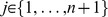by setting for , for , and 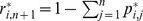. Pointwise entropy 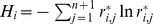measures the variability in nucleotides found to be base-paired with in the Boltzmann ensemble of low energy structures. The pointwise entropy without the probing data is computed similarly using the probabilities . To reflect the nature of the probing data, we modified this definition as follows. Define the binary pointwise entropy at position by . Binary entropy measures the uncertainty in the th nucleotide being paired or unpaired, reflecting the signal detected by probing data. Similar computations were done with (the base pairing probabilities without the integration of the weights). The Morgan-Higgs structural diversity is defined by 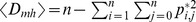, where is defined by . Similar computations were done with .

RNAsc is guaranteed to improve agreement with shape data

In this section, we show that on average, the ensemble of low energy secondary structures produced by our method yields a footprinting pattern that more closely resembles the pattern from input experimental shape data; in particular, we prove that the expected distance from (normalized) shape data for the ensemble of low energy structures (our algorithm) is strictly less than the expected distance from shape data for the Boltzmann ensemble of low energy structures (McCaskill's algorithm). First, we require some definitions. All secondary structures considered in this section will be tacitly assumed to be secondary structures of the RNA molecule . Each secondary structure can be assigned a binary sequence so that if the nucleotide is paired and otherwise. Given experimental shape data yielding probabilities , where is the probability that nucleotide is unpaired, the distance of to is defined by:

(9)

The shape weight of is defined to be

(10)

The weighted partition function then becomes

(11)

The Boltzmann probability of secondary structure is defined by

(12)

and the weighted Boltzmann probabity is defined by

(13)

Define the critical distance by

(14)

Note that does not depend on any particular secondary structure , although it does depend on and of course the input RNA sequence . It follows from definitions that for any secondary structure ,

(15)

and strict inequalities hold as well. Indeed, since the exponential function is increasing, we have if and only if

Multiplying each side by , the above inequality can be written as

from which (15) follows. Similarly,

(16)

Next, define the expected distance between , obtained by normalizing shape data, and the ensemble of low energy structures as follows:

(17)

Similarly, define the SHAPE weighted expected distance between and the ensemble of low energy structures by

(18)

Let represent the sorted distances between all secondary structures of , for given normalized shape data . Here denotes the total number of secondary structures. Note that there may be many distinct secondary structures that have a given distance to ; i.e. possibly many distinct for which . Let be the largest index such that ; it follows that and . Let [resp. ] consist of those secondary structures , such that [resp. ]; in other words

Theorem 1: For any given RNA sequence and normalized SHAPE data , .

Proof:

To justify the inequality, note that for , , hence for , we have . On the other hand, for , , hence for , we also have . Finally, the last line follows from the fact that and are both probability distributions, hence . This completes the proof that .

The above theorem can be generalized; however, we first require some notation. The weighted partition function , weighted Boltzmann probability , and weighted expected distance were respectively defined in Equations (11),(13), and (18). When we wish to make the weighting parameter explicit, we instead write , and . The following theorem shows that as the parameter increases, the expected distance to normalized shape data decreases:

Theorem 2: For any given RNA sequence , normalized SHAPE data and , ; moreover, strict inequalities hold as well.

The proof the the theorem can be found in File S1.

Quadratic time computation of expected distance from shape data

Given RNAsc parameter , recall that we defined the -expected distance between , obtained by normalizing shape data, and the ensemble of low energy structures by

(19)

In the main text, we wrote , instead of when .

In trying to compute by definition, we seemingly require the sum over exponentially many secondary structures, or at least to approximate this sum by summing over a reprentative sample of structures, sampled from the low energy ensemble. This is not necessary. Here, we show how to compute from the base pairing probabilities , thus leading to a quadratic time algorithm.

By definition,

where is denotes the indicator function. Now for any fixed ,

is equal to

(20)

Since , it follows that Equation (20) is equal to

(21)

It follows that

The values are computed in quadratic time from McCaskill's algorithm, and subsequently stored in an array. If follows that can be computed in quadratic time.

Since RNAstructure of Deigan et al. [15] takes unnormalized shape data in the range from to , we define the expected distance between unnormalized shape data and structure to be

(22)

where denotes the unnormalized shape data at position . The expected distance between unnormalized shape data and the ensemble of low energy structures computed by RNAstructure with incorporated shape data by

(23)

Scrutiny of the proof just given yields an efficient computation of

(24)

Since the approach in [15] only considers stacked base pairs, it seems very likely that , where denotes the expected distance from shape data for the Boltzmann ensemble of low energy structures after the incorporation of the shape pseudo energy terms as in [15]. Indeed, the expected distance we obtain between unnormalized input shape data and the computed probabilities demonstrates this fact (see Table 1).

Results

In this section we present the benchmarking results for our algorithm RNAsc, a novel algorithm that recalibrates probing data as probabilities of nucleotides being unpaired and integrates this information as ‘soft constraints’ into the computation of minimum free energy secondary structure (see Methods). Furthermore, we present a direct comparison of in-line probing data and shape data for yeast asp-tRNA.

Analysis of shape and in-line probing for structure prediction

In order to directly characterize how well shape data reflects RNA secondary structure, we compared normalized shape data with base pairing status, as determined from crystallographic or NMR structures. We define shape distance to equal the difference between normalized shape reactivity (see Methods), scaled from to (see section Normalization of shape) and binary base pairing status, with 0 for paired, 1 for unpaired, as derived from NMR or crystal structure. Using shape data for S. cerevisiae apartyl-tRNA [25], HCV IRES [15], bI3 group I intron p456 [33], E. coli phenylalanine-tRNA [26], E. coli 5S RNA [26], and Fusobacterium nucleatum glycine riboswitch [26], we computed shape distance at each nucleotide. We observed that at many positions the shape distance has an absolute value greater than 0.5, thus indicating a significant difference between shape reactivity and the actual secondary structure. We refer to these positions as discrepancies. Over the the set of RNAs we examined, between of the total data corresponded to such discrepancies (Fig. 3 and File S1). Many factors can account for these discrepancies, including differences between the crystal structure and the ensemble of structures in solution, potential tertiary contacts, and differential reactivity to the chemical agent.

Figure 3. Shape discrepancies.

Distribution of shape discrepancies in yeast asp-tRNA (top) and E. coli phe-tRNA (bottom). shape data for asp-tRNA [resp. phe-tRNA] from the Weeks Lab [25] [resp. Das Lab [26]]. Using crystal structure as ‘gold standard’, red squares indicate locations where the absolute value of the difference of shape data and crystal structure (1 unpaired, 0 paired) exceeds 0.5. The plots on the right show the distribution of the discrepancy in shape as well as the error rate.

To assess whether an alternative experimental method might yield data that more accurately reflects the secondary structure, we performed in-line probing on the S. cereviseae aspartyl-tRNA, for which shape data is available [25]. Like shape, in-line probing is a measure of backbone flexibility, where nucleotides in loops and other unpaired regions are generally more reactive than those that are base-paired [34]. In-line probing takes advantage of the spontaneous transesterification reactions responsible for RNA degradation that occur only when the O from one nucleotide and the O of the next align in a 180 degree conformation around the phosphate. This conformation does not occur in the A-form helix, thus protecting linkages within the helix from cleavage. In-line probing and shape are thus likely to yield similar, but not equivalent data [35].

Our analysis indicates that in-line probing and shape reactivity profiles are quite distinct from one another. See Fig. 4 for a comparison of shape and in-line probing profiles and File S1 for shape reactivity profiles of other RNA molecules.

Figure 4. Comparison of In-line probing and shape.

Distribution of reactivities of data from in-line probing (A) and shape (B). In-line probing reactivities were determined using SAFA [24] and then normalized to range , in order to be comparable with shape reactivities. Histograms suggest that in-line probing signal is more diffuse than that from shape. The fraction of base-pairs in asp-tRNA is which could be used to estimate the threshold shape moderate reactivity.

The signal from in-line probing is significantly more diffuse than that from shape, and the error rate, as calculated above for shape, is significantly higher ( vs. ). Thus shape is a better reflection of secondary structure than in-line probing, at least in the case of asp-tRNA.

Integrating shape and in-line probing data into our new algorithm RNAsc also shows that shape has an edge over in-line probing. The structures predicted by RNAsc for yeast asp-tRNA using in-line probing and shape data are both identical to the crystal structure. However, one measure of the robustness of the data in the context of our secondary structure prediction algorithm RNAsc is the range of the scaling parameter over which the correct structure can be recovered. Recall that is a weight parameter (see section Boltzmann Weights for details). We conducted a search for parameter for yeast asp-tRNA, using both in-line probing data and shape data. We found that when using in-line probing data, RNAsc produced the target structure for asp-tRNA only for a very narrow range of , while when using shape data, this range was much larger (see Fig. 5). See Fig. 6 for a heat map of in-line vs. shape reactivity for asp-tRNA.

Figure 5. Optimal parameter value.

The plots show heat maps displaying ppv () as a function of parameter for RNAsc with data from shape and in-line probing (asp-tRNA ). Note the much larger area for good parameter choices when using shape data, rather than in-line probing data. This data suggests that shape data is more robust than in-line probing data, when used in computing MFE structure with RNAsc. Computations were done at 37C.

Figure 6. Heat maps of in-line probing and shape.

Heat maps illustrating differences between in-line probing (left) and shape (right) analysis of the yeast asp-tRNA. Nucleotides are colored corresponding to cumulative activities described in Figure 3, where the least reactive of bases are black ( of bases are paired in the crystal structure), the most reactive of bases are red, and the next most reactive are yellow. Gray bases are bases for which there is no data available.

In a second analysis, we compared the pointwise entropy at each nucleotide using no data, shape data, and in-line probing data (see Fig. 7). We observe that shape data decreases the average entropy more than in-line probing data. However, we also observe that there are positions where the in-line probing decreases the entropy more than shape, suggesting that combinations of different experimental approaches may be able to yield additional information.

Figure 7. Pointwise entropies.

Pointwise entropy of yeast asp-tRNA, computed from RNAsc using shape data (red squares), in-line probing (blue diamonds), and using no probing data (black circles). Average pointwise entropies: 0.210 (shape data), 0.267 (in-line probing), 0.269 (no data). As expected, by integrating either shape or in-line probing data into RNAsc, the variability (entropy) decreases; however, it appears that variability (entropy) is decreased more by shape than by in-line probing data – again, suggesting that shape data is more robust than in-line probing data when used with RNAsc.

Validation of RNAsc

Using shape data from the Weeks Lab, we tested RNAsc on aspartyl-tRNA from S. cerevisiae, domain II of the hepatitis C virus internal ribosomal entry site (HCV IRES), and the P546 domain of the bI3 group I intron, from E. coli. Additionally, using shape data from the Das Lab, we tested RNAsc on E. coli phenylalanine tRNA (phe-tRNA), E. coli 5S ribosomal RNA (5S rRNA), and the glycine riboswitch from F. nucleatum with PDB code 3P49. As ‘gold standard’ structures, we used NMR structure for P546, and X-ray structures for remaining RNAs. Parameter used for RNAsc is , determined by search (see Fig. 5) to optimize sensitivity (proportion of true positives that are correctly identified) and positive predictive value (proportion of positive results that are true positives). Slippage of [15], [36] is not allowed, contrary to benchmarking results of some authors. Here, slippage [36] means that if base pair is in the true structure, then the base pair is counted as “correctly” predicted, if one of the base pairs , , , appears in the predicted structure – we do not allow slippage in the results of this paper.

Table 1 presents a comparison of RNAsc with RNAstructure, including a comparison of structural variation in the ensemble of low energy structures. This variation is computed by pointwise entropy and Morgan-Higgs structural diversity (see Methods). The table shows that the low energy ensemble, as computed by RNAsc with integration of shape data, has intermediate variation between that computed by RNAstructure with and without shape data. The fact that RNAstructure with incorporated shape data computes an ensemble of structures with less variation appears to be expected, given the parameters used in the algorithm of Deigan et al. [15].

As explained in Deigan et al. [15], RNAstructure incorporates shape data by including a pseudo free energy term

(25)

for a nucleotide position . In the source code RNAstructure, it is clear that the pseudo free energy term is applied only for positions involved in a stacked base pair. The optimal values for slope and -intercept are obtained by grid search when maximizing structure prediction accuracy on certain known structures. Optimal slope and intercept values reported in [15] are and kcal/mol.

We now show that the smaller structural variation in the RNAstructure ensemble appears to be an artifact of the magnitude of parameters . Consider the two most extreme cases: (1) position in structure is base-paired, but shape reactivity is a maximum, (2) position in structure is not paired, but shape reactivity is a minimum.

Suppose that position is in a base-stacked region but the shape reactivity at position is , a maximum, though there are sometimes shape reactivities larger than . With the default parameters for , the pseudo free energy contribution of RNAstructure is , an energetic penalty. This penalty is quite large, given the fact that the largest (in absolute value) free energy contribution for base stacking is kcal/mol [37]. Under the same assumptions, RNAsc would have a pseudo free energy of , also an energetic penalty, yet much smaller than that of RNAstructure.

Suppose now that position is in a loop region but the shape reactivity at position is , the least possible value. Using the default parameters kcal/mol, the pseudo free energy contribution of RNAstructure, if applied in this case, would then be . This value, paradoxically, would be an energetic bonus, although the predicted structure disagrees with shape data! It is presumably for this reason that Deigan et al. do not apply any pseudo free energy term to nucleotide positions located in a loop region. In contrast, under the same assumptions, RNAsc would have a pseudo free energy of , again a penalty – moreover, the same penalty of kcal/mol is applied in each of the cases (1) and (2) just discussed.

From these illustrative examples, it is suggestive that structural variability, as measured by pointwise entropy and structural diversity, in the low energy ensemble calculated by RNAstructure is higher than that of the RNAsc low energy ensemble, due to the magnitude of the parameters used in RNAsc.

Note that the average relative decrease in expected distance of the computed probabilities to shape data from RNAstructure to RNAsc is . In fact the expected distance of the computed probabilities to shape increases for RNAstructure and decreases for RNAsc after the incorporation of shape in each case. Apart from the ‘self-consistent’ nature of our algorithm, not shared by RNAstructure, the demonstrable expected distance of the computed probabilities to shape data provided by our approach, indicates that we account more fully for the shape data. It is worth mentioning that for higher values of the predicted Boltzmann probabilities can be made to agree very closely with the experimental values (strong self-consistency). Fig. 8 shows a plot of the expected distance of the computed probabilities to shape data for increasing values of – see Methods for a proof. Note however that since the experimental probabilities (or normalized shape values) are generally not in perfect agreement with the native structure, we took the closeness of the predicted structure to the native structure as a measure for choosing the parameter .

Figure 8. Expected distance of predicted probabilities with normalized shape data.

The figure shows a plot of the expected distance between normalized experimental shape values and the low energy Boltzmann ensemble, as computed by RNAsc. The -axis depicts increasing values of RNAsc parameter , while the -axis depicts expected distance . The curves confirm the statement of Theorem 2, which states that as increases, the expected distance decreases. The figure also shows that for higher values of , can be made to agree very closely . The expected distances of the predicted probabilities with unnormalized shape values for RNAstructure are , , and for asp-tRNA, HCV, and P546 respectively using optimal parameter values ( and ).

We believe RNAsc may be helpful long-term in elucidating the nature of discrepancies between shape and the native structure. As in any experimental protocol, there is a Gaussian error term; however, our data (not shown) indicates that shape discrepancy is positively correlated with high pointwise entropy. Indeed, it seems plausible that a region of the RNA molecule which fluctuates due to thermal motion, thus having higher pointwise entropy, might entail a more variable accessibility for the chemical probe NMIA, thus causing a greater shape discrepancy with the X-ray structure. The program RNAsc allows the user to determine such regions of high pointwise entropy, and to see the structure variability in that region by sampling. It may be possible to confirm or refute our hypothesis concerning the non-Gaussian nature of shape discrepancy (“error”), by performing additional shape probing experiments at lower temperatures. It follows that RNAsc could prove to be a valuable tool in this line of research.

Discussion

Widespread accessibility of quantitative RNA structural mapping techniques and medium- to high-throughput quantification of the data have motivated the development of computational tools to predict structures from such information. The integration of experimental data as “constraints” in the thermodynamic algorithm when computing minimum free energy (MFE) structure can significantly improve the accuracy of RNA structure prediction. However, such methods are also dependent on the quality of the data used for the constraints [26]. It is worth mentioning that the errors in our algorithm RNAsc are directly related to the errors in the experimental data. Fig. 9 shows shape distance to the native structure at the nucleotides where the secondary structure is predicted incorrectly for glycine riboswitch. As can be seen, the shape distances to the native structure are very large for out of the incorrectly predicted positions. Thus the prediction errors are due to the quality of the input data rather than limitations of the algorithm.

Figure 9. Errors in the prediction of the secondary structure of glycine riboswitch by RNAsc.

On the -axis, nucleotide positions are displayed, where the algorithm predicts the structure incorrectly. The -axis represents the shape distance to the native structure at the given nucleotide. A shape distance with absolute value indicates an error.

Two recent approaches towards overcoming this error include the iterative ‘sample and select’ approach of Quarrier et al. [38] and the ‘mutate and map’ strategy of Kladwang et al. [30]. The ‘sample and select’ strategy involves multiple mapping, followed by a simple filtering step, which removes the suboptimal structures (sampled from the low energy ensemble using the Sfold software [39]) that are incompatible with mapping data. In contrast, the ‘mutate and map’ strategy involves high-throughput structural probing of all single-nucleotide mutants, resulting in 2D shape data, followed by a computation of the minimum free energy structure, in which pseudo-energy base stacking terms have been added that correspond to Z-scores from 2D shape data. Although high-throughput ‘mutate and map’ strategies [30], using either shape -CE (capillary electrophoresis) or shape -Seq [40], provide very high secondary structure prediction accuracy, such methods also represent a significant increase in both experimental manipulation and cost that is often not warranted for more specific studies. Especially in such cases, we believe that our method, RNAsc, may be the tool of choice. On the other hand, the ‘mutate and map’ strategy can be normalized in such a way as to obtain base pairing probabilities. Since shape experiments can potentially probe tertiary interactions (as mentioned in the previous section), not only could we obtain probabilities for secondary interactions and canonical base pairs, but also for tertiary and long range interactions as well as non-canonical base pairs. These probabilities can later be used as input to algorithms such as Probknot [41] or even to a Maximum Weight Matching algorithm [42] to predict pseudoknotted structures and non-canonical base pairs. We are currently pursuing this line of research.

Supporting Information

File S1

Supplementary information.

(PDF)

Funding Statement

No current external funding sources for this study.

References

- 1. Washietl S (2010) Sequence and structure analysis of noncoding RNAs. Methods in molecular biology (Clifton, NJ) 609: 285–306. [DOI] [PubMed] [Google Scholar]
- 2.Garey M, Johnson D (1990) Computers and Intractability: A Guide to the Theory of NPCompleteness. W.H. Freeman & Co., 338 pages pp. New York.
- 3. Lyngso RB, Pedersen CN (2000) RNA pseudoknot prediction in energy-based models. J Comput Biol 7: 409–427. [DOI] [PubMed] [Google Scholar]
- 4. Zuker M, Stiegler P (1981) Optimal computer folding of large RNA sequences using thermodynamics and auxiliary information. Nucleic Acids Res 9: 133–148. [DOI] [PMC free article] [PubMed] [Google Scholar]
- 5. Tinoco JI, Bustamante C (1999) How RNA folds. Journal of Molecular Biology 293: 271–281. [DOI] [PubMed] [Google Scholar]
- 6. Banerjee A, Jaeger J, Turner D (1993) Thermal unfolding of a group I ribozyme: The lowtemperature transition is primarily disruption of tertiary structure. Biochemistry 32: 153–163. [DOI] [PubMed] [Google Scholar]
- 7. Cho SS, Pincus DL, Thirumalai D (2009) Assembly mechanisms of RNA pseudoknots are determined by the stabilities of constituent secondary structures. Proc Natl Acad Sci USA 106: 17349–17354. [DOI] [PMC free article] [PubMed] [Google Scholar]
- 8. Bailor MH, Sun X, Al-Hashimi HM (2010) Topology links RNA secondary structure with global conformation, dynamics, and adaptation. Science 327: 202–206. [DOI] [PubMed] [Google Scholar]
- 9. Wilkinson K, Merino E, Weeks K (2005) RNA SHAPE chemistry reveals nonhierarchical interactions dominate equilibrium structural transitions in tRNAAsp. J Am Chem Soc 127: 4659–4667. [DOI] [PubMed] [Google Scholar]
- 10. Zuker M (2003) Mfold web server for nucleic acid folding and hybridization prediction. Nucleic Acids Res 31 (13) 3406–3415. [DOI] [PMC free article] [PubMed] [Google Scholar]
- 11. Hofacker I, Fontana W, Stadler P, Bonhoeffer L, Tacker M, et al. (1994) Fast folding and comparison of RNA secondary structures. Monatsch Chem 125: 167–188. [Google Scholar]
- 12.Mathews D, Turner D, Zuker M (2000) Secondary structure prediction. In: Beaucage S, Bergstrom D, Glick G, Jones R, editors, Current Protocols in Nucleic Acid Chemistry, New York: John Wiley & Sons. pp. 11.2.1–11.2.10.
- 13. Xia T, SantaLucia J, Burkard M, Kierzek R, Schroeder S, et al. (1999) Thermodynamic parameters for an expanded nearest-neighbor model for formation of RNA duplexes with Watson-Crick base pairs. Biochemistry 37: 14719–35. [DOI] [PubMed] [Google Scholar]
- 14. Mathews DH, Disney MD, Childs JL, Schroeder SJ, Zuker M, et al. (2004) Incorporating chemical modification constraints into a dynamic programming algorithm for prediction of RNA secondary structure. Proc Natl Acad Sci USA 101: 7287–7292. [DOI] [PMC free article] [PubMed] [Google Scholar]
- 15. Deigan KE, Li TW, Mathews DH, Weeks KM (2009) Accurate SHAPE-directed RNA structure determination. Proc Natl Acad Sci USA 106: 97–102. [DOI] [PMC free article] [PubMed] [Google Scholar]
- 16. Kertesz M, Wan Y, Mazor E, Rinn JL, Nutter RC, et al. (2010) Genome-wide measurement of RNA secondary structure in yeast. Nature 467: 103–107. [DOI] [PMC free article] [PubMed] [Google Scholar]
- 17. Merino EJ, Wilkinson KA, Coughlan JL, Weeks KM (2005) RNA structure analysis at single nucleotide resolution by selective 2′-hydroxyl acylation and primer extension (SHAPE). J Am Chem Soc 127: 4223–4231. [DOI] [PubMed] [Google Scholar]
- 18.Wilkinson K, Merino E, Weeks K (2006) Selective 20-hydroxyl acylation analyzed by primer extension (SHAPE): quantitative RNA structure analysis at single nucleotide resolution. NATURE PROTOCOLS-ELECTRONIC EDITION- 1: 1610. [DOI] [PubMed]
- 19. Wilkinson KA, Gorelick RJ, Vasa SM, Guex N, Rein A, et al. (2008) High-throughput SHAPE analysis reveals structures in HIV-1 genomic RNA strongly conserved across distinct biological states. PLoS Biol 6: e96. [DOI] [PMC free article] [PubMed] [Google Scholar]
- 20. Ban N, Nissen P, Hansen J, Moore PB, Steitz TA (2000) The complete atomic structure of the large ribosomal subunit at 2.4 A resolution. Science 289: 905–920. [DOI] [PubMed] [Google Scholar]
- 21. Novikova IV, Hennelly SP, Sanbonmatsu KY (2012) Structural architecture of the human long non-coding RNA, steroid receptor RNA activator. Nucleic Acids Research [DOI] [PMC free article] [PubMed] [Google Scholar]
- 22. Mandal M, Boese B, Barrick J, Winkler W, Breaker R (2003) Riboswitches control fundamental biochemical pathways in Bacillus subtilis and other bacteria. Cell 113 (5) 577–586. [DOI] [PubMed] [Google Scholar]
- 23. Meyer M, Roth A, Chervin S, Garcia G, Breaker R (2008) Confirmation of a second natural preQ1 aptamer class in Streptococcaceae bacteria. RNA 14: 685–695. [DOI] [PMC free article] [PubMed] [Google Scholar]
- 24. Das R, Laederach A, Pearlman SM, Herschlag D, Altman RB (2005) SAFA: semi-automated footprinting analysis software for high-throughput quantification of nucleic acid footprinting experiments. RNA 11: 344–354. [DOI] [PMC free article] [PubMed] [Google Scholar]
- 25. Wilkinson K, Merino E, Weeks K (2005) RNA SHAPE chemistry reveals nonhierarchical interactions dominate equilibrium structural transitions in tRNAAsp transcripts. Journal of the American Chemical Society 127: 4659–4667. [DOI] [PubMed] [Google Scholar]
- 26. Kladwang W, Vanlang CC, Cordero P, Das R (2011) Understanding the Errors of SHAPE-Directed RNA Structure Modeling. Biochemistry 50: 8049–8056. [DOI] [PMC free article] [PubMed] [Google Scholar]
- 27. McCaskill J (1990) The equilibrium partition function and base pair binding probabilities for RNA secondary structure. Biopolymers 29: 1105–1119. [DOI] [PubMed] [Google Scholar]
- 28. Matthews D, Sabina J, Zuker M, Turner D (1999) Expanded sequence dependence of thermodynamic parameters improves prediction of RNA secondary structure. J Mol Biol 288: 911–940. [DOI] [PubMed] [Google Scholar]
- 29. Forties RA, Bundschuh R (2010) Modeling the interplay of single-stranded binding proteins and nucleic acid secondary structure. Bioinformatics 26: 61–67. [DOI] [PubMed] [Google Scholar]
- 30. Kladwang W, Cordero P, Das R (2011) A mutate-and-map strategy accurately infers the base pairs of a 35-nucleotide model RNA. RNA 17: 522–534. [DOI] [PMC free article] [PubMed] [Google Scholar]
- 31. Zuker M (1989) On finding all suboptimal foldings of an RNA molecule. Science 244: 48–52. [DOI] [PubMed] [Google Scholar]
- 32. Higgs PG (1996) Overlaps between RNA secondary structures. Physical Review Letters 76: 704–707. [DOI] [PubMed] [Google Scholar]
- 33. Duncan C, Weeks K (2008) Shape analysis of long-range interactions reveals extensive and thermodynamically preferred misfolding in a fragile group i intron RNA. Biochemistry 47: 8504–8513. [DOI] [PMC free article] [PubMed] [Google Scholar]
- 34. Soukup G, Breaker R (1999) Relationship between internucleotide linkage geometry and the stability of RNA. RNA 5: 1308–1325. [DOI] [PMC free article] [PubMed] [Google Scholar]
- 35. Dann CE, Wakeman C, Sieling C, Baker S, Irnov I, et al. (2007) Structure and mechanism of a metal-sensing regulatory RNA. Cell 130: 878–892. [DOI] [PubMed] [Google Scholar]
- 36. Mathews D (2005) Predicting a set of minimal free energy RNA secondary structures common to two sequences. Bioinformatics 15: 2246–2253. [DOI] [PubMed] [Google Scholar]
- 37. Turner DH, Mathews DH (2010) Nndb: the nearest neighbor parameter database for predicting stability of nucleic acid secondary structure. Nucleic acids research 38: D280–2. [DOI] [PMC free article] [PubMed] [Google Scholar]
- 38. Quarrier S, Martin J, Davis-Neulander L, Beauregard A, Laederach A (2010) Evaluation of the information content of RNA structure mapping data for secondary structure prediction. RNA 16: 1108–1117. [DOI] [PMC free article] [PubMed] [Google Scholar]
- 39. Ding Y, Chan CY, Lawrence CE (2004) Sfold web server for statistical folding and rational design of nucleic acids. Nucleic Acids Res 32: 0. [DOI] [PMC free article] [PubMed] [Google Scholar]
- 40. Lucks JB, Mortimer SA, Trapnell C, Luo S, Aviran S, et al. (2011) Multiplexed RNA structure characterization with selective 2′-hydroxyl acylation analyzed by primer extension sequencing (SHAPE-Seq). Proceedings of the National Academy of Sciences of the United States of America 108: 11063–11068. [DOI] [PMC free article] [PubMed] [Google Scholar]
- 41. Bellaousov S, Mathews DH (2010) Probknot: fast prediction of RNA secondary structure including pseudoknots. RNA (New York, NY) 16: 1870–1880. [DOI] [PMC free article] [PubMed] [Google Scholar]
- 42. Tabaska J, Cary R, Gabow H, Stormo G (1998) An RNA folding method capable of identifying pseudoknots and base triples. Bioinformatics 14: 691–699. [DOI] [PubMed] [Google Scholar]
- 43. Reuter JS, Mathews DH (2010) RNAstructure: software for RNA secondary structure prediction and analysis. BMC Bioinformatics 11: 129. [DOI] [PMC free article] [PubMed] [Google Scholar]
Associated Data
This section collects any data citations, data availability statements, or supplementary materials included in this article.
Supplementary Materials