

Abstract
Differences in the toxicity of ambient particulate matter (PM) due to varying particle composition across locations may contribute to variability in results from air pollution epidemiologic studies. Though most studies have used PM mass concentration as the exposure metric, an alternative which accounts for particle toxicity due to varying particle composition may better elucidate whether PM from specific sources is responsible for observed health effects. The oxidative potential (OP) of PM < 10 μm (PM10) was measured as the rate of depletion of the antioxidant reduced glutathione (GSH) in a model of human respiratory tract lining fluid. Using a database of GSH OP measures collected in greater London, U.K. from 2002 to 2006, we developed and validated a predictive spatiotemporal model of the weekly GSH OP of PM10 that included geographic predictors. Predicted levels of OP were then used in combination with those of weekly PM10 mass to estimate exposure to PM10 weighted by its OP. Using cross-validation (CV), brake and tire wear emissions of PM10 from traffic within 50 m and tailpipe emissions of nitrogen oxides from heavy-goods vehicles within 100 m were important predictors of GSH OP levels. Predictive accuracy of the models was high for PM10 (CV R2=0.83) but only moderate for GSH OP (CV R2 = 0.44) when comparing weekly levels; however, the GSH OP model predicted spatial trends well (spatial CV R2 = 0.73). Results suggest that PM10 emitted from traffic sources, specifically brake and tire wear, has a higher OP than that from other sources, and that this effect is very local, occurring within 50–100 m of roadways.
Introduction
Several recent epidemiologic studies have reported heterogeneity in effect estimates of fine particles from different sources,1−8 some of which are supported by recent toxicological studies.9−11 Though less extensive, studies also document heterogeneity in effect estimates of PM10.12,13 Many studies have found increased respiratory7 and cardiac health risks from exposures to traffic14,15 or PM from traffic sources2,4,6,16−18 suggesting that traffic-related PM is more toxic than PM from other sources. Differential toxicity of PM from different sources may explain some of the observed heterogeneity in results from epidemiologic studies that used PM mass concentration as the metric of exposure.
Understanding the differential toxicity of PM from different sources has been identified as a priority for environmental health research.19 These efforts are complicated by the diverse physical and chemical properties of PM, many of which can be measured but whose relevance in the toxicity of PM is poorly understood.20 Oxidative potential (OP) of PM offers a convenient means of integrating over these complex characteristics, providing a summary measure indicative of PM toxicity that is directly relevant to pollutant behavior in the human lung.21−24 OP can be considered a measure of the inherent capacity of PM to induce oxidative stress in the lung.
Although models have been developed to predict exposure to traffic-related PM, to date, there are no models of exposure to the oxidizing properties of PM that can be applied in epidemiological studies. Our objectives were 2-fold: (1) To establish the feasibility of using an approach similar to land-use regression (LUR) alone, or in combination with spatiotemporal modeling, to predict the weekly average OP of PM10 in greater London, U.K.; and (2) To generate an exposure metric reflecting OP-weighted PM10 that could be compared to PM10 mass concentration in epidemiologic investigations.
Materials and Methods
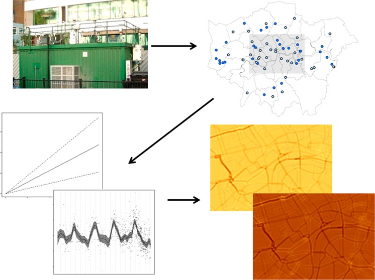
Using a database of measured OP and PM10 levels, together with information about the surroundings of the monitoring sites derived from a geographic information system (GIS), we developed predictive geostatistical models to estimate weekly average location-specific levels of the OP of PM10 as well as PM10 mass concentrations from 2002 to 2006. Because our intent was to predict OP levels during the monitored time period, our analysis focused on determining spatial predictors of OP, with purely temporal predictors to be identified in a separate analysis.
Air Pollutant Data
PM10 concentrations are routinely measured at many ambient air monitoring sites across greater London using Tapered Element Oscillating Microbalance (TEOM; Rupprecht & Patashnick model 1400A, New York) monitors; data from 66 sites were available for this analysis. Hourly TEOM data were reported in units of μg m–3 and corrected for volatilization losses using a multiplier of 1.3 for 2002 and a volatilization-correction model for 2003–2006.25
OP Data
OP was measured based on the collected particles’ ability to deplete the antioxidant reduced glutathione (GSH) in an acellular model of respiratory-tract lining fluid.21,22 The methods used to measure GSH OP are described in detail elsewhere.23,26,27 Briefly, suspensions of PM collected on TEOM filters at a standardized concentration (50 μg mL–1) were incubated in an antioxidant solution for 4 h. Particle-free, negative (inert black-carbon particles), as well as positive (residual oil fly ash) controls were run in parallel to assess auto-oxidative losses and allow for standardization between batches. The amount of GSH lost over the 4 h period relative to a particle-free control was calculated per μg PM10.
Data on GSH OP were available from 34 monitoring sites across the study domain of greater London (shown in Supporting Information Figure S1), though not continuously at all sites. Valid data were available for 25% of all possible weeks. TEOM filters were changed on an irregular schedule based on filter loading, with about half of the sampling periods less than two weeks in duration (median: 15 days; 25th and 75th percentiles are 7 and 28 days, respectively (n = 841)). Thus, each filter provided an OP measurement integrated over the sampling period, but the sampling periods did not necessarily coincide in time at different sites. To obtain weekly average OP values with concurrent start and stop days across the 34 monitoring sites, we assigned the multiday integrated OP measurements to each day of the corresponding sampling period and derived weekly average values by taking the weighted average (in proportion to days of measurement) of daily values that occurred within each calendar week, excluding weeks with less than 4 valid days. Further details on the temporal realignment of the OP data can be found in the Supporting Information.
Geographic Data
The geographic coordinates of each monitoring site on the British National Grid were used in combination with data on building and traffic density to derive geographic covariates describing the surroundings of each monitoring location. Building density variables were provided by colleagues at the Bartlett School of Architecture, University College London, U.K. These data were derived from postcode level information from the Ordnance Survey MasterMap Topography Layer28 and Cities Revealed Topography layer.28 From these data sources, the following variables were calculated at 100, 250, 500, and 1000 m radii around the monitoring sites: (1) the “built-space” ratio (proportion of land covered with buildings or structures), (2) the artificial coverage ratio (proportion of land covered with human-made surfaces), (3) the green coverage ratio (proportion of land covered with green surfaces), (4) the water coverage ratio (proportion of land covered with inland water), and (5) the urban volumetric density (built-space ratio multiplied by the average height).
Data on traffic density and emissions were obtained from the London Atmospheric Emissions Inventory29 for the year 2005. For each road segment in the inventory, emissions of nitrogen oxides (NOX) and PM10 from road traffic were calculated based on (1) the Annual Average Daily Total (AADT) traffic count for 2005, and (2) the mixture of vehicle types present on London roads in 11 categories. These categories were further refined using data on the proportions of Euro classes within each vehicle category using data from the U.K. Department for Transport’s national stock model and, for taxis and buses, from the Greater London Authority. For this analysis the traffic emissions data were collapsed into three groups: heavy-goods vehicles, light-goods vehicles, and “other” vehicles (buses, cars, motorcycles, and taxis). This collection of road location, traffic density, and emissions data provided a highly spatially resolved database on (1) cumulative traffic levels and (2) vehicular NOX and PM10 emissions with enough spatial accuracy to reliably estimate gradients within 50 m of the monitoring site. To calculate cumulative traffic levels, we multiplied the AADT for each road segment by the segment length within 50, 100, and 200 m buffers, by vehicle group and total. For vehicular emissions of NOX and PM10, we calculated tailpipe NOX and PM10 emissions, by vehicle group and total, within 50, 100, and 200 m buffers. Additionally, for PM10 only, we calculated emissions from brake and tire wear within the same buffers. The data on traffic density and NOX and PM10 tailpipe emissions, as well as PM10 from brake and tire wear, were also summed, by vehicle group and for all road and nonroad sources combined, within 1 km2 grid cells to provide area-level aggregate measures.
A hybrid emissions-dispersion/regression model of annual-average PM10 levels with high spatial resolution has been previously developed for use in greater London and is described in detail elsewhere.30,31 This model used emissions data from the London Atmospheric Emissions Inventory29 and incorporated near-road impacts and meteorology using ADMS-Roads; we used it to obtain annual-average PM10 levels for 2003, 2004, and 2006 on a 20 m grid over the study domain of central London. We then bilinearly interpolated these annual-average values to each prediction location, and averaged the resulting three values by location to create a spatially varying covariate that described long-term average PM10 levels with high spatial resolution.
Statistical Models
GSH OP
We developed a geostatistical spatiotemporal model to predict weekly average GSH OP levels at unmeasured locations anywhere within the study domain throughout 2002–2006. To do this, we evaluated several modeling approaches of varying complexity, from simple space-time models using penalized splines and linear effects of GIS covariates, to approaches which further added time-varying smooth spatial trends, nonlinear covariate effects, and different assumptions with respect to the correlation structure among within-site errors.
We used cross-validation (CV) at the location level rather than the location-week level to describe the predictive accuracy of each candidate model using the following steps. First, we divided the data set into two parts by leaving out the monitoring data for a given location. Next, we fitted the candidate model to the reduced data set containing data from all locations except the left-out location. We then used that fitted model to predict weekly values at the left-out location, and repeated this process for each of the monitoring sites. The CV R2 was calculated as the squared Pearson correlation between the measured values at a given location and the model predictions when that location was left out of the model fitting process. Because we performed CV at the location level, the presence of successive weekly data points at a given site did not influence CV results. The degree of model overfitting was assessed as the difference between the model R2 and the CV R2. The candidate model with the highest CV R2 was used as the final prediction model. Because our focus was on modeling spatial variation, in instances where candidate models differed only with respect to the spatial covariates included, we averaged the measurements and model predictions across time (one mean per site and year and one mean per site) to obtain and compare annual-average and spatial CV R2 values, respectively. Temporal CV R2 values were similarly calculated by first averaging weekly predictions across locations (one mean per week) and then comparing week-specific average measurements and predictions. We assessed bias in model predictions using the slope from linear regression of the left-out measurements against model predictions, and examined the precision of model predictions by calculating the square root of the mean of the squared prediction errors (RMSPE), where prediction errors were defined as predicted minus measured values. We also calculated the mean fractional bias (MFB) and mean fractional error (MFE) of model predictions according to the formulas provided in the Supporting Information.
We used a generalized additive mixed model (GAMM) to describe spatial and temporal variation in weekly average GSH OP levels measured across greater London from 2002 to 2006. GAMMs were fit using the gamm () function in the mgcv package32−34 for R35 with smoothing parameter selection performed using the maximum likelihood method. We also used linear mixed effects models with a compound symmetric covariance structure for preliminary identification of GIS covariates using PROC MIXED in SAS v9.2 (Cary, NC), selecting those that had the lowest (best) AIC or most significant (smallest) p-value in separate models. Further model selection was performed in several phases, described below. First, we evaluated an initial space-time GAMM,
| 1 |
where GSH OPit is the weekly average at location i (i = 1...I; I = 34) and week t, and g(si) is a two-dimensional spatial smooth function of the projected coordinates (easting and northing) at location i specified using thin-plate penalized splines (basis dimension k = 0.9I). The week index t ranged from 1 to T = 247 (corresponding to the weeks beginning December 31, 2001 and September 18, 2006, respectively). Though weekly averages were available at ≥4 sites for most weeks (73%), for two weeks no data were available. Because of this missing data in time, we did not specify an intercept for each time period αt. Instead, we specified h(t) as a thin-plate spline (basis dimension k = 0.9T) which represents the adjusted smoothed mean value across all sites for each week. Our choice of basis dimension was as large as practical, to allow the data to determine the complexity of the fitted functions32−34. eit is assumed a mean-zero, Gaussian-distributed error term with constant variance σ2e. σ2eλitt′ specifies covariances between errors at location i, with λitt′ parametrized as to induce either a compound symmetric (fixed correlation between measurements at the same site and no correlation between measurements at different sites: λitt′ = σ1/σ2e) or an autoregressive (AR(1); exponentially decreasing correlation in time between measurements at the same site and no correlation between measurements at different sites: λitt′ = ρ|t–t′|) covariance structure.
Next, we removed the spatial and temporal terms in separate models. To the “best” (highest CV R2) of these three models (later referred to as the “referent” model), we then added GIS covariates one at a time in separate models (“univariate” models). In these univariate models, we evaluated both linear terms (βzi) and nonlinear smooth functions (f(zi); using a thin-plate spline basis with basis dimension k = 4) of each GIS covariate zi. From these models, we obtained a set of GIS covariates that improved predictive accuracy compared to the referent model, and only these GIS covariates were considered in later stages of model selection.
Next, we included these selected GIS covariates in ‘multivariable’ GAMMs, removing any nonsignificant (i.e., p > 0.05) covariates one at a time, beginning with the least significant. We also evaluated these models for parsimony, removing each remaining term one at a time, and keeping only those that improved predictive accuracy. We then evaluated whether the effects of the remaining GIS covariates varied seasonally (i.e., winter, spring, summer, autumn) by including seasonal interaction terms, again removing nonsignificant terms. Finally, we evaluated whether any spatiotemporal interaction remained in the data, which could potentially explain additional variability in the outcome, by adding seasonal spatial terms, gseason(si), and weekly spatial terms, gt(si), separately, to the model. Details regarding space-time interaction and different spatial models (thin-plate spline smoothing vs ordinary and simple kriging) are given in the Supporting Information.
To obtain predicted weekly average GSH OP at unmeasured locations, we first generated the selected GIS covariates at prediction locations and then used the fitted GAMMs. GIS and meteorological predictors were truncated to their range among the monitoring locations to avoid extrapolation. Prediction involved only the fixed-effects of the model; the nonzero covariance assumed among the within-site errors provided control for overfitting of the smooth terms and other fixed-effects.
PM10
We also developed a geostatistical model to predict weekly average PM10 concentrations at unmeasured locations anywhere within the study domain of central London, U.K. throughout 2002–2006. Because high-resolution spatial information on annual-average PM10 levels was available from the hybrid emissions-dispersion/regression model developed for greater London,30,31 the goal of the weekly model was to leverage this rich spatial data and explicitly model weekly temporal variation. To do this, we used a similar approach as for GSH OP, but considered for inclusion as a covariate only the three-year mean of annual-average PM10 predictions from the hybrid emissions-dispersion/regression model (M0306HED). Cross-validation, model specification with respect to spatiotemporal structure, and model prediction were performed for the PM10 model in the same way as for GSH OP.
Exposure Metrics
Thus, two exposure metrics can be
calculated from the predictive models: (1) PM10![]() and (2) GSH OP-weighted PM10
and (2) GSH OP-weighted PM10![]() . This formulation allows direct comparison of the effects
of ÊPM10 and ÊGSH OP in health effect analyses
because the PM10 mass concentration component is the same
in both. Modeling (GSH OP)(PM10) in units of μg m–3 would not afford this direct comparison.
. This formulation allows direct comparison of the effects
of ÊPM10 and ÊGSH OP in health effect analyses
because the PM10 mass concentration component is the same
in both. Modeling (GSH OP)(PM10) in units of μg m–3 would not afford this direct comparison.
Results
GSH OP data were available at 34 monitoring sites (2118 weekly averages), and PM10 data at 66 sites (12 043 weekly averages), from 2002 to 2006. Weekly average GSH OP values in units of OP μg–1 were approximately normally distributed, with 0%, 25%, 50%, mean, 75%, and 100% values of 0, 0.45, 0.72, 0.76, 1.05, and 1.78, respectively, and an arithmetic standard deviation (SD) of 0.39. Weekly average PM10 levels in units of μg m–3 were approximately log-normally distributed, with 0%, 25%, 50%, geometric mean, 75%, and 100% values of 8.2, 20.3, 25.7, 26.0, 32.8, and 101.3, respectively, and a geometric SD of 1.43.
GSH OP
Upon inclusion in univariate models, nine of the 10 GIS predictors identified in preliminary linear mixed effect models improved predictive accuracy compared to the referent model (listed in Supporting Information Table S1), which included only the intercept, α, and the smooth term for time trend, h(t), as fixed effects. Interestingly, the inclusion of a smooth spatial term, g(si), decreased predictive accuracy and was not included. Thus, the model relied upon geographic covariates to explain spatial variation in GSH OP. Nonlinear spline terms did not increase predictive accuracy for any of the GIS covariates; therefore, linear effects were used.
In multivariable models, only NOX tailpipe emissions from heavy-goods vehicles within 50 m (NOXHGV50) and PM10 brake and tire wear emissions from all vehicles within 50 m (PM10BT50) remained significant and maximized CV performance. We then investigated the spatial scale over which the impacts of both of these covariates varied by using larger buffers of 100 m instead of 50 m. For PM10BT50, the original 50 m buffer performed best (CV R2 = 0.42 for 50 m vs 0.39 for 100 m), whereas for NOXHGV50 a 100 m buffer (NOXHGV100) performed slightly better than the 50 m buffer (CV R2 = 0.424 for 100 m vs 0.417 for 50 m). Allowing the linear slope to change seasonally further improved predictive accuracy slightly (Supporting Information Table S1; CV R2 = 0.44 with seasonal interaction and 0.42 without) for PM10BT50, but did not for NOXHGV100 (data not shown). Thus, the final GSH OP prediction model was of the following form:
| 4 |
where the residual term eit (compound symmetric, chosen based on the CV R2) and h(t) are specified as above in eq 1 and where z1i is NOXHGV100, z2i is PM10BT50, and the xSeason terms are dummy variables for each season. A Mg year–1 increase in NOXHGV100 was associated with a 0.12 decrease in GSH OP μg–1. Increased PM10BT50 was positively associated with GSH OP in each season, with this effect largest in summer and smallest in autumn, with estimated values of 7.3, 11.0, 11.3, and 5.6 for winter, spring, summer, and autumn, respectively (all in GSH OP μg–1 for a Mg year–1 increase in PM10). Table S2 in the Supporting Information contains further details on the model parameters. The reduced slope in autumn and the peaks in the time trend term corresponding to the autumn season suggest that GSH OP levels are higher but less spatially variable (i.e., less local) during this time of year. Despite the moderate correlation (Pearson’s r = 0.70) between PM10BT50 and NOXHGV100, only PM10BT50 was significant in univariate models (slope (SE) of 4.86 (1.22) with no seasonal interaction). Upon inclusion in the same multivariable model, the sign of the slope for NOXHGV100 became negative (Supporting Information Table S2). This may reflect changes in the mixture of PM10 components due to differences in vehicle composition, suggesting that locations with higher NOX tailpipe emissions from heavy-goods vehicles have lower levels of GSH OP-active PM10 components per unit PM10 mass.
The model explained about half of the variability in weekly GSH OP levels (model R2 = 0.52), and thus, in comparison with the CV R2, overfitting of the model was moderately well controlled for at 8.1%. The smooth function for time trend used 40.5 degrees of freedom (df) and showed a marked seasonal pattern, with an increase in late autumn of each year (Supporting Information Figure S2), typically around October or November.
Predictive accuracy was moderate for weekly levels (CV R2 = 0.44), but increased considerably when evaluating only spatial variability (Table 1; spatial CV R2 = 0.73), and also increased when predicting only temporal variability (Table 1; temporal CV R2 = 0.71). Also, predictive accuracy for weekly levels was increased among sites with at least 88 measurements (CV R2 = 0.54), and when comparing annual-averages (Table 2; CV R2 = 0.67). We found little bias in weekly model predictions (linear regression slope = 0.97 and MFB = 7.8%), but only moderate to poor precision (Table 1; RMSPE = 0.29 OP μg–1 or 39% of the mean; MFE = 37.4%). However, precision improved considerably for spatial predictions (Table 1; RMSPE = 0.13 OP μg–1 or 17% of the mean). Additionally, predictive accuracy and precision by season, year, tertiles of urban volumetric density, and site type are shown in Table 1. Additional details regarding model performance by these categories can be found in the Supporting Information.
Table 1. Model Performance Statistics for GSH OP and PM10 Models.
| pollu-tant | grouping | cross-validation R2a | RMSPEab | ||||||||
|---|---|---|---|---|---|---|---|---|---|---|---|
| GSH OP | across all | 0.44 | 0.29 | ||||||||
| by season | winter | spring | summer | autumn | winter | spring | summer | autumn | |||
| 0.25 | 0.34 | 0.39 | 0.34 | 0.30 | 0.28 | 0.29 | 0.32 | ||||
| by year | 2002 | 2003 | 2004 | 2005 | 2006 | 2002 | 2003 | 2004 | 2005 | 2006 | |
| 0.39 | 0.48 | 0.41 | 0.47 | 0.34 | 0.30 | 0.25 | 0.29 | 0.29 | 0.31 | ||
| by urban volu-metric densityc | low | medium | high | low | medium | high | |||||
| 0.34 | 0.50 | 0.42 | 0.31 | 0.27 | 0.30 | ||||||
| by site type | urban background | roadside | kerbside | urban background | roadside | curbside | |||||
| 0.45 | 0.36 | 0.13 | 0.25 | 0.32 | 0.31 | ||||||
| annual- meand | 0.67 | 0.14 | |||||||||
| spatiale | 0.73 | 0.13 | |||||||||
| temporale | 0.71 | 0.12 | |||||||||
| PM10 | across all | 0.83 | 4.62 | ||||||||
| by season | winter | spring | summer | autumn | winter | spring | summer | autumn | |||
| 0.85 | 0.86 | 0.81 | 0.73 | 4.24 | 5.15 | 4.12 | 4.56 | ||||
| by year | 2002 | 2003 | 2004 | 2005 | 2006 | 2002 | 2003 | 2004 | 2005 | 2006 | |
| 0.68 | 0.92 | 0.79 | 0.78 | 0.73 | 4.68 | 4.74 | 4.30 | 4.16 | 4.93 | ||
| by urban volu-metric densityc | low | medium | high | low | medium | high | |||||
| 0.74 | 0.82 | 0.87 | 5.51 | 4.73 | 4.27 | ||||||
| by site type | urban background | suburban | roadside | curbside | urban background | suburban | roadside | curbside | |||
| 0.88 | 0.90 | 0.80 | 0.78 | 3.64 | 3.43 | 4.99 | 5.74 | ||||
| annual- meand | 0.67 | 2.68 | |||||||||
| spatiale | 0.61 | 2.65 | |||||||||
| temporale | 0.76 | 2.16 | |||||||||
Across weekly averages (2118 at 34 locations for GSH OP and 12 041 at 66 locations for PM10). For PM10, two high values at two sites were removed as outliers.
RMSPE is root mean squared prediction error. Units are OP μg–1 for GSH OP and μg m–3 for PM10.
Defined using tertiles of the urban volumetric density (see text for definition) within 500 m. For PM10, across only 6710 weekly averages at the 34 locations where GSH OP was also measured.
To calculate “annual-mean” values, measurements and predictions were averaged by year at each site with at least 31 weeks of data per year.
To calculate “spatial” values, measurements and predictions were averaged over time at each site with at least 40 weeks of data; similarly “temporal” refers to averaging over locations for all weeks for which measurements were available.
Table 2. GSH OP Model Performance Statistics by Emission Type and Vehicle Group Categories.
| cross-validation R2 |
RMSPEa |
||||
|---|---|---|---|---|---|
| PM10 emissions within 50 m | vehicle group | weeklyb | spatialc | weeklyb | spatialc |
| tailpipe | total | 0.40 | 0.63 | 0.31 | 0.15 |
| heavy-goods | 0.35 | 0.51 | 0.32 | 0.17 | |
| light-goods | 0.19 | 0.00 | 0.36 | 0.26 | |
| otherd | 0.41 | 0.65 | 0.30 | 0.14 | |
| brake and tire wear | total | 0.44 | 0.73 | 0.29 | 0.13 |
| heavy-goods | 0.28 | 0.15 | 0.34 | 0.22 | |
| light-goods | 0.36 | 0.51 | 0.32 | 0.17 | |
| otherd | 0.43 | 0.71 | 0.30 | 0.13 | |
RMSPE is root mean squared prediction error. Units are OP μg–1.
Across 2118 weekly averages at 34 locations.
To calculate “spatial” values, measurements and predictions were averaged over time at sites with at least 40 weeks of data.
“Other” category includes buses, cars, motorcycles, and taxis.
To further explore the impact of emission type (tailpipe vs brake and tire wear) and vehicle group (heavy-goods, light-goods, and “other”) of PM10 emissions within 50 m on spatial variation in GSH OP, we substituted covariates from each of these categories in the final GSH OP prediction model. The results in Table 2 show that the strongest of these predictors was brake and tire wear PM10 emissions from all vehicles (“total” category) from the final GSH OP prediction model.
However, among individual vehicle groups, the “other” category (buses, cars, motorcycles, and taxis) had the highest predictive accuracy, again suggesting differences in the composition of PM10 emissions from roadways with high “other” vehicle traffic (with likely a higher proportion of petrol (gasoline)-fueled vehicles) vs those with higher heavy-goods traffic (with likely a higher proportion of diesel-fueled vehicles). These alternate models were identical except that different spatial predictors were included; therefore, differences in predictive accuracy were more pronounced when comparing spatial rather than weekly CV R2 values.
The maps in Supporting Information Figure S3 display the spatial and temporal variability in predicted GSH OP levels in central London. Using a conventional sums of squares decomposition, the variability in weekly predictions at the grid points shown in Figure S3 was 12% spatial and 87% temporal, with the remainder attributable to rounding error. Maps showing the impact of the seasonally varying effects of the PM10 brake and tire wear emissions covariate on the spatial variability in modeled GSH OP are presented in Supporting Information Figure S4.
PM10
The form of the space-time PM10 prediction model was
| 5 |
where the terms are as above in eq 1, z1i is M0306HED in μg m–3, and eit ∼ N(0, σ2e). Again the untransformed outcome performed as well as alternatives, and therefore PM10 was modeled on the original scale.
The referent model for PM10 included only an intercept, α, and a smooth function for time trend, h(t), as fixed-effects (Supporting Information Table S1), and did not include a smooth spatial term g(si). Inclusion of M0306HED improved predictive accuracy compared to the referent model (CV R2 = 0.74 without and 0.83 with). Because the hybrid emissions-dispersion/regression model included the influence of roadway emissions and other small scale effects, it, not surprisingly, described micro- to middle-scale (0–500 m) spatial variation in PM10 levels better than spatial smoothing splines alone. As was the case for GSH OP, a linear covariate effect performed better than a nonlinear spline. The slope for this covariate, M0306HED, was near unity (1.01; Supporting Information Table S2), indicating that predictions from the hybrid emissions-dispersion/regression model were properly scaled to the measurements. However, as distinct from the GSH OP model, removing the compound symmetric covariance structure did not substantially increase the df in the smooth function for time trend h(t) (219.7 with and 220.0 without), did not increase overfitting (0.2% with and without), and had no substantive effect on predictive accuracy (CV R2 = 0.83 with and without). Due to this finding, we used the simpler GAM without control for correlation among within-site errors for prediction of weekly PM10 levels. Despite this, no consistent pattern of autocorrelation in adjacent lag periods was observed in the model residuals and autocorrelation values were generally small (r < 0.25 for lags greater than two weeks).
Predictive accuracy decreased somewhat when predicting only spatial variability compared to weekly levels of PM10 (Table 1; spatial CV R2 = 0.61 among sites with at least 40 weeks of data), but increased for temporal predictions, highlighting the importance of temporal versus spatial variability for PM10 (Table 1; temporal CV R2 = 0.76). Also, predictive accuracy was high for annual averages (CV R2 = 0.67). We found very little bias in weekly model predictions (linear regression slope = 1.00 and MFB = 1.2%), and moderate precision (Table 1; RMSPE = 4.62 μg m–3 or 17% of the mean; MFE = 12.4%). Model precision improved when comparing only spatial variability (Table 1; RMSPE = 2.65 μg/m3 or 10% of the mean). The PM10 model performed well across seasons, years and in highly as well as less urban areas.
Weekly predicted values across the 66 sites ranged from 10.3 to 100.8 μg/m3, whereas measured levels ranged from 8.1 to 101.3 μg m–3. The model explained about 84% of the variability in weekly PM10 levels (Supporting Information Table S1), and thus, in comparison with the CV R2, overfitting of the model was very well controlled for at 0.2%. M0306HED was quite influential on predicted weekly PM10 values; weekly PM10 predictions varied by 62% across the range of M0306HED relative to the mean.
The maps in Supporting Information Figure S6 display the spatial and temporal variability in predicted PM10 concentrations in central London. Higher PM10 concentrations near both major and minor roadways are evident (Supporting Information Figure S6), as is the importance of temporal compared to spatial variability: Using a conventional sums of squares decomposition, the variability in predicted values at these grid points was 7% spatial and 93% temporal.
GSH OP-Weighted PM10
The maps in Figure 1 show the spatial and temporal variability in ÊGSH OP in central London, U.K.
Figure 1.
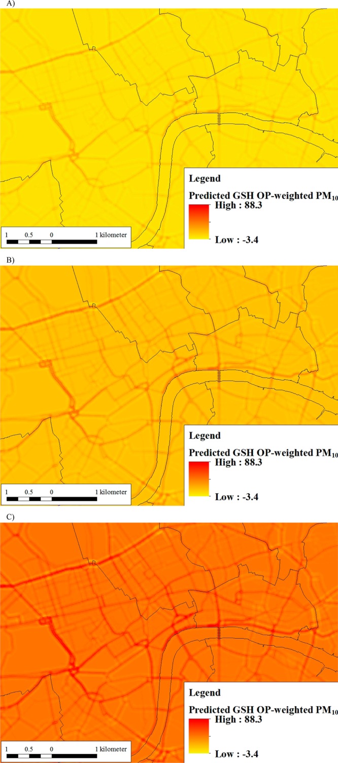
Maps of predicted GSH OP-weighted PM10 levels in OP m–3 in a selected area of central London, U.K. (A) Lowest week (beginning December 6, 2004; values ranged from −3.4 to 29.2 OP m–3); (B) Mean across 2002–2006 (values ranged from 3.0 to 50.4 OP m–3); (C) Highest week (beginning July 21, 2003; values ranged from 22.0 to 88.3 OP m–3).
The influence of PM10 brake and tire wear emissions and NOX tailpipe emissions near roadways is again evident. Again using a conventional sums of squares decomposition, the variability in weekly predictions was 19% spatial and 79% temporal, with the 2% remainder attributable to noise. Multiplying predicted GSH OP by predicted PM10 to calculate ÊGSH OP increased the spread of the distribution compared to that of PM10 alone (interquartile range is 80% of the median for ÊGSH OP vs 42% for ÊPM10), and will likely increase the exposure contrast available for epidemiologic studies, though the extent of this result will depend on the proportion of the population living near (<50–100 m) roadways. Perhaps most importantly, the correlation between ÊGSH OP and ÊPM10 is only moderate (Spearman’s r = 0.62), indicating that weighting by OP affects the relative ranking of location-specific PM exposure estimates.
Discussion
Our results suggest that PM10 at locations with higher brake and tire wear emissions from vehicles has higher GSH OP compared to that at other locations, and that this effect is extremely local, occurring within 50 m of roadways. This suggests that “fresh” and very local PM10 brake and tire wear emissions may be more toxic with respect to OP than PM10 from other sources, perhaps due to the metal content in brake material. This suggestion is supported by our CV results, where very local (within 50 m) PM10 brake and tire wear emissions proved to be the most effective predictor of spatial variation in GSH OP levels.
We have demonstrated the predictive accuracy of geostatistical models of weekly GSH OP and PM10 levels within the study domain of greater London, U.K. from 2002 to 2006. For GSH OP, the results demonstrate the ability of LUR using traffic emissions and geographic road network data to explain spatial variability in measured GSH OP levels. In addition to spatial variability, our results also demonstrate substantial temporal variability in GSH OP and PM10, as described by the temporal smoothing terms in our models; these trends in time would not have been captured using LUR alone. Our model for GSH OP was able to explain a significant portion of the variability in GSH OP levels (model R2 = 0.52), and CV results showed that predictive accuracy for GSH OP at left-out monitoring locations (substituting for unmeasured residential locations) was moderate (CV R2 = 0.44). Predictions from the GSH OP and PM10 models can be combined to define an exposure metric which quantitatively describes the inherent capacity of PM to induce oxidative stress in the lung. Use of such an exposure metric, having more relevance to impacts on the lung which in turn could drive local and systemic inflammation,24 has the potential to reduce exposure error in studies of PM health effects and allow greater precision in health-effect estimates.
We observed seasonal variation in the effect of the PM10 brake and tire wear emissions covariate on GSH OP levels. This variation may in part be due to seasonal changes in the vehicular emissions themselves, but is more likely due to different meteorological trends during the seasons, or to changes in the composition of PM, perhaps as a consequence of interactions with other seasonal pollutants. The higher slopes for the PM10 brake and tire wear emissions covariate in spring and summer seasons indicate that GSH OP levels increase more sharply near roadways during these seasons than others. This may be the result of reaction with secondary pollutants that are higher during those periods of the year with increased solar radiation, such as ozone, of seasonal changes in the metal content of PM, or of increased resuspension of PM near roadways in drier, windier seasons.
We also observed a negative association between NOX tailpipe emissions from heavy-goods vehicles within 100 m and GSH OP, though for this term the effect size was smaller than for PM10 brake and tire wear emissions. While somewhat counterintuitive, this negative association may suggest that PM10 emissions from roadways with greater heavy-goods vehicle traffic exhibit differences in composition that influence GSH OP. Interestingly, this finding is consistent with locations where elemental carbon would be expected to contribute a higher proportion of PM10 mass (those with higher heavy-goods traffic indicated by NOX emissions) corresponding to lower GSH OP. We note that NOX tailpipe emissions are likely reflecting variation in PM components, rather than causing a direct effect on GSH OP, because OP analyses were done on PM collected on the sampling filters; gaseous NOX would have passed through the sampling filters and therefore not affected later analyses.
LUR has been widely used to describe spatial variability in measured pollutant levels.36,37 Our GSH OP analysis is distinct from typical LUR models, however, in that we are modeling a characteristic of collected PM10 (its GSH OP in units of OP μg–1) rather than a pollutant concentration, and in that, using a generalized additive mixed model, we explicitly model temporal variation (rather than averaging it out) while accounting for autocorrelation among the within-site errors.
Nonetheless, our study has several limitations. One is that only estimates of the weekly average GSH OP were available due to the irregular sampling time periods. Even though this feature of the data could induce errors resulting in too much smoothing of the estimated time trend and increased autocorrelation in model residuals, we found only little to moderate evidence of autocorrelation. We were not able to determine to what extent the varying duration of the sampling periods affected the GSH OP measurements, but note that the effects of GIS covariates in our model are estimated based on spatial comparisons, rather than temporal; the high spatial CV R2 (0.73) would suggest that the model describes these spatial patterns quite well. Also, despite our use of a site-specific random effect, the data may not be missing completely at random and thus the spatiotemporal imbalance in our data may have induced bias in the model effect estimates. Additionally, the TEOM monitor involves heating of sample filters which, could have resulted in an underestimation of GSH OP due to a loss of oxidatively active volatile species. However, GSH OP has been found to be similar when collected by TEOM compared to other methods that retain the volatile component of PM10.30 Also, GSH OP is not a direct measure of particle toxicity. Rather, it only captures the OP of components in collected PM that do not require cellular metabolism to induce oxidative stress, and so may underestimate the total oxidative stress burden of inspired PM. Additionally, geographic data on roadway locations in greater London, U.K. do not necessarily reflect only spatial variation in traffic-related air pollutant emissions, but rather may also reflect to some extent spatial variation in other sources which may occur at the same locations, such as tobacco smoke from sidewalks lining busy roads. However, those emissions are unlikely to be highly correlated with cumulative traffic levels and are likely unaffected by changes in the vehicle group on a given roadway. Thus, given our finding of a linear relationship between GSH OP and traffic emissions specific to a given emission type (brake and tire wear), and that the strength of this relationship varied by emission type, this explanation seems implausible.
Given our finding of very local (within 50–100 m) spatial variation in GSH OP levels, future investigations should focus on modeling weekly or even daily wind-direction dependent traffic-related air pollutant emissions as a predictor of GSH OP. Such a predictor may be able to explain additional variation in GSH OP levels, and may further elucidate the link between traffic-related air pollutant emissions, the OP of PM, and the time-scale and magnitude of their impact on human health. Also, future research on the relationships between GSH OP and specific PM10 components related to traffic sources is warranted. Epidemiologic studies attempting to assess exposures to oxidant-weighted PM should focus on capturing variation in OP on smaller spatial scales (0–100 m) than typically used for routine ambient monitoring networks.
Acknowledgments
This independent research was commissioned and funded by the Policy Research Programme in the U.K. Department of Health as part of the Health Effects of Outdoor and Indoor Air Pollution initiative. The research was also supported by the National Institute for Health Research (NIHR) Biomedical Research Centre based at Guy’s and St Tomas’ NHS Foundation Trust and King’s College London. The views expressed are those of the author(s) and not necessarily those of the NHS, the NIHR, or the U.K. Department of Health. C.T. was funded by the U.K. Economic and Social Research Council RES-064-27-0026. We thank Anna Mavrogianni, Bartlett School of Architecture, University College London, for providing data on building density, and Ben Armstrong, London School of Hygiene and Tropical Medicine, and Christopher Paciorek, Harvard School of Public Health, for thoughtful reviews of the early manuscript.
Supporting Information Available
Two tables and five figures and tables referred to in the text, as well as additional details on the methods and results concerning alternate spatial statistical approaches and on the seasonal variability in GSH OP. This material is available free of charge via the Internet at http://pubs.acs.org.
The authors declare no competing financial interest.
Author Present Address
† Department of Social and Environmental Health Research, London School of Hygiene & Tropical Medicine, London, U.K.
Author Present Address
‡ Environmental Research Group, MRC-HPA Centre for Environment and Health, King’s College London, London, U.K.
Supplementary Material
References
- Laden F.; Neas L. M.; Dockery D. W.; Schwartz J. Association of fine particulate matter from different sources with daily mortality in six U.S. cities. Environ. Health Perspect. 2000, 108(10), 941–947. [DOI] [PMC free article] [PubMed] [Google Scholar]
- Lanki T.; de Hartog J. J.; Heinrich J.; Hoek G.; Janssen N. A. H.; Peters A.; Stölzel M.; Timonen K. L.; Vallius M.; Vanninen E.; Pekkanen J. Can we identify sources of fine particles responsible for exercise-induced ischemia on days with elevated air pollution? The ULTRA study. Environ. Health Perspect. 2006, 114(5), 655–660. [DOI] [PMC free article] [PubMed] [Google Scholar]
- Ostro B.; Feng W. Y.; Broadwin R.; Green S.; Lipsett M. The effects of components of fine particulate air pollution on mortality in California: Results from CALFINE. Environ. Health Perspect. 2007, 115(1), 13–19. [DOI] [PMC free article] [PubMed] [Google Scholar]
- Sarnat J. A.; Marmur A.; Klein M.; Kim E.; Russell A. G.; Sarnat S. E.; Mulholland J. A.; Hopke P. K.; Tolbert P. E. Fine particle sources and cardiorespiratory morbidity: An application of chemical mass balance and factor analytical source-apportionment methods. Environ. Health Perspect. 2008, 116(4), 459–466. [DOI] [PMC free article] [PubMed] [Google Scholar]
- Franklin M.; Koutrakis P.; Schwarz J. The role of particle composition on the association between PM2.5 and mortality. Epidemiol. 2008, 19(5), 680–689. [DOI] [PMC free article] [PubMed] [Google Scholar]
- Zanobetti A.; Franklin M.; Koutrakis P.; Schwartz J.. Fine particulate air pollution and its components in association with cause-specific emergency admissions. Environ. Health 2009, 8 (58). [DOI] [PMC free article] [PubMed] [Google Scholar]
- Ostro B.; Roth L.; Malig B.; Marty M. The effects of fine particle components on respiratory hospital admissions in children. Environ. Health Perspect. 2009, 117(3), 475–480. [DOI] [PMC free article] [PubMed] [Google Scholar]
- Bell M. L.; Belanger K.; Ebisu K.; Gent J. F.; Joo Lee H.; Koutrakis P.; Leaderer B. P. Prenatal exposure to fine particulate matter and birth weight: Variations by particulate constituents and sources. Epidemiol. 2010, 21(6), 884–891. [DOI] [PMC free article] [PubMed] [Google Scholar]
- Lippmann M.; Chen L. C. Health effects of concentrated ambient air particulate matter (CAPs) and its components. Crit. Rev. Toxicol. 2009, 39(10), 865–913. [DOI] [PubMed] [Google Scholar]
- Schwarze P. E.; Ovrevik J.; Lag M.; Refsnes M.; Nafstad P.; Hetland R. B.; Dybing E. Particulate matter properties and health effects: Consistency of epidemiological and toxicological studies. Human Exp. Toxicol. 2006, 25(10), 559–579. [DOI] [PubMed] [Google Scholar]
- Cho S.-H.; Tong H; McGee J. K.; Baldauf R. W.; Krantz Q. T.; Gilmour M. I. Comparative toxicity of size-fractionated airborne particulate matter collected at different distances from an urban highway. Environ. Health Perspect. 2009, 117(11), 1682–1689. [DOI] [PMC free article] [PubMed] [Google Scholar]
- Samoli E.; Analitis A.; Touloumi G.; Schwartz J.; Anderson H. R.; Sunyer J.; Bisanti L.; Zmirou D.; Vonk J. M.; Pekkanen J.; Goodman P.; Paldy A.; Schindler C.; Katsouyanni K. Estimating the exposure-response relationships between particulate matter and mortality within the APHEA multicity project. Environ. Health Perspect. 2005, 113(1), 88–95. [DOI] [PMC free article] [PubMed] [Google Scholar]
- Peng R. D.; Dominici F.; Pastor-Barriuso R.; Zeger S. L.; Samet J. M. Seasonal analyses of air pollution and mortality in 100 U.S. Cities. Am. J. Epidemiol. 2005, 161(6), 585–594. [DOI] [PubMed] [Google Scholar]
- Peters A.; von Klot S.; Heier M.; Trentinaglia I.; Hormann A.; Wichmann H. E.; Lowel H. Exposure to traffic and the onset of myocardial infarction. N. Engl. J. Med. 2004, 351(17), 1721–1730. [DOI] [PubMed] [Google Scholar]
- Tonne C.; Melly S.; Mittleman M.; Coull B.; Goldberg R.; Schwartz J. A case-control analysis of exposure to traffic and acute myocardial infarction. Environ. Health Perspect. 2007, 115(1), 53–57. [DOI] [PMC free article] [PubMed] [Google Scholar]
- Effects of Long-Term Exposure to Traffic-Related Air Pollution on Respiratory and Cardiovascular Mortality in the Netherlands: The NLCS-AIR Study; Health Effects Institute: Boston, MA, 2009; http://pubs.healtheffects.org/view.php?id=302. [PubMed] [Google Scholar]
- von Klot S.; Gryparis A.; Tonne C.; Yanosky J. D.; Coull B. A.; Goldberg R. J.; Lessard D.; Melly S. J.; Suh H. H.; Schwartz J. Elemental carbon exposure at residence and survival after acute myocardial infarction. Epidem. 2009, 20(4), 547–554. [DOI] [PubMed] [Google Scholar]
- Brugge D. L.; Durant J. L.; Rioux C.. Near-highway pollutants in motor vehicle exhaust: A review of epidemiologic evidence of cardiac and pulmonary health risks. Environ. Health 2007, 6 (23). [DOI] [PMC free article] [PubMed] [Google Scholar]
- Committee on Research Priorities for Airborne Particulate Matter. Research Priorities for Airborne Particulate Matter I: Immediate Priorities and a Long-Range Research Portfolio; National Research Council (NRC), National Academy Press: Washington, DC, 1998. [PubMed] [Google Scholar]
- Pope C. A. III; Dockery D. W. Health effects of fine particulate air pollution: Lines that connect. J. Air Waste Manage. Assoc. 2006, 56, 709–742. [DOI] [PubMed] [Google Scholar]
- Kelly F. J.; Cotgrove M.; Mudway I. S. Respiratory tract lining fluid antioxidants: The first line of defence against gaseous pollutants. Cent. Eur. J. Public Health 1996a, 4(Suppl), 11–14. [PubMed] [Google Scholar]
- Kelly F. J.; Blomberg A.; Frew A.; Holgate S. T.; Sandstrom T. Antioxidant kinetics in lung lavage fluid following exposure of humans to nitrogen dioxide. Am. J. Respir. Crit. Care Med. 1996b, 154(6), 1700–1705. [DOI] [PubMed] [Google Scholar]
- Kunzli N.; Mudway I. S.; Gotschi T.; Shi T.; Kelly F. J.; Cook S.; Burney P.; Forsberg B.; Gauderman J. W.; Hazenkamp M. E.; Heinrich J.; Jarvis D.; Norback D.; Payo-Losa F.; Poli A.; Sunyer J.; Borm P. J. A. Comparison of oxidative properties, light absorbance, and total and elemental mass concentration of ambient PM2.5 collected at 20 European sites. Environ. Health Perspect. 2006, 114(5), 684–690. [DOI] [PMC free article] [PubMed] [Google Scholar]
- Ayers J. G.; Borm P.; Cassee F. R.; Castranova V.; Donaldson K.; Ghio A.; Harrision R. M.; Hider R.; Kelly F.; Kooter I. M.; Marano F.; Maynard R. L.; Mudway I.; Nel A.; Sioutas C.; Smith S.; Baeza-Squiban A.; Cho A.; Duggan S.; Froines J. Evaluating the Toxicity of airborne particulate matter and nanoparticles by measuring oxidative stress potential—A workshop report and consensus statement. Inhalation Toxicol. 2008, 20(1), 75–99. [DOI] [PubMed] [Google Scholar]
- Green D. C.; Fuller G. W.; Baker T. Development and validation of the volatile correction model for PM10—An empirical method for adjusting TEOM measurements for their loss of volatile particulate matter. Atmos. Environ. 2009, 43(13), 2132–2141. [Google Scholar]
- Godri K. J.; Green D. C.; Fuller G. W.; Dall’Osto M.; Beddows D. C.; Kelly F. J.; Harrison R. M.; Mudway I. S. Particulate oxidative burden associated with firework activity. Environ. Sci. Technol. 2010, 44(21), 8295–8301. [DOI] [PubMed] [Google Scholar]
- Mudway I. S.; Stenfors N.; Duggan S. T.; Roxborough H.; Zielinski H.; Marklund S. L.; Blomberg A.; Frew A. J.; Sandstromb T.; Kelly F. J. An in vitro and in vivo investigation of the effects of diesel exhaust on human airway lining fluid antioxidants. Arch. Biochem. Biophys. 2004, 423(1), 200–212. [DOI] [PubMed] [Google Scholar]
- Ordnance Survey MasterMap; http://www.ordnancesurvey.co.uk/oswebsite/products/os-mastermap/topography-layer/index.html (accessed September 13, 2010).
- London Atmospheric Emissions Inventory 2003, 2nd Annual Report; Greater London Authority: London, UK, 2006; http://static.london.gov.uk/mayor/environment/air_quality/docs/laei_2003.pdf. [Google Scholar]
- Kelly F. J.; Anderson H. R.; Armstrong B.; Atkinson R.; Barratt B.; Beevers S.; Cook D.; Derwent R.; Duggan S.; Green D.; Mudway I. S.; Wilkinson P.. The impact of the congestion charging scheme on air quality in London: Part 2. Analysis of the oxidative potential of particulate matter Res. Rep. - Health Eff. Inst. 2011, 155, 73–144. [PubMed] [Google Scholar]
- Tonne C.; Beevers S.; Armstrong B. G.; Kelly F.; Wilkinson P. Air pollution and mortality benefits of the London Congestion Charge: Spatial and socioeconomic inequalities. Occup. Environ. Med. 2008, 65(9), 620–627. [DOI] [PubMed] [Google Scholar]
- Wood S. N. Stable and efficient multiple smoothing parameter estimation for generalized additive models. J. Am. Stat. Assoc. 2004, 99(467), 673–686. [Google Scholar]
- Wood S. N. Fast stable direct fitting and smoothness selection for generalized additive models. J. R. Stat. Soc. (B) 2008, 70(3), 495–518. [Google Scholar]
- Wood S. N.Generalized Additive Models: An Introduction with R; Chapman and Hall/CRC: Boca Raton, Florida, U.S.A., 2006. [Google Scholar]
- R Development Core Team. R: A Language and Environment for Statistical Computing; R Foundation for Statistical Computing: Vienna, Austria, 2009; ISBN 3-900051-07-0, http://www.R-project.org. [Google Scholar]
- Jerrett M.; Arain A.; Kanaroglou P.; Beckerman B.; Potoglou D.; Sahsuvaroglu T.; Morrison J.; Giovis C. A review and evaluation of intraurban air pollution exposure models. J. Exposure Anal. Environ. Epidemiol. 2005, 15(2), 185–204. [DOI] [PubMed] [Google Scholar]
- Hoek G.; Beelen R.; de Hoogh K.; Vienneau D.; Gulliver J.; Fischer P.; Briggs D. A review of land-use regression models to assess spatial variation of outdoor air pollution. Atmos. Environ. 2008, 42(13), 7561–7578. [Google Scholar]
Associated Data
This section collects any data citations, data availability statements, or supplementary materials included in this article.