BDflex: A method for efficient treatment of molecular flexibility in calculating protein-ligand binding rate constants from Brownian dynamics simulations

Abstract

A method developed by Northrup [J. Chem. Phys. 80, 1517 (1984)]10.1063/1.446900 for calculating protein-ligand binding rate constants (k_a) from Brownian dynamics (BD) simulations has been widely used for rigid molecules. Application to flexible molecules is limited by the formidable computational cost to treat conformational fluctuations during the long BD simulations necessary for k_a calculation. Here, we propose a new method called BDflex for k_a calculation that circumvents this problem. The basic idea is to separate the whole space into an outer region and an inner region, and formulate k_a as the product of k_E and ${\overline{\eta }}_{\mathrm{d}}$, which are obtained by separately solving exterior and interior problems. k_E is the diffusion-controlled rate constant for the ligand in the outer region to reach the dividing surface between the outer and inner regions; in this exterior problem conformational fluctuations can be neglected. ${\overline{\eta }}_{\mathrm{d}}$ is the probability that the ligand, starting from the dividing surface, will react at the binding site rather than escape to infinity. The crucial step in reducing the determination of ${\overline{\eta }}_{\mathrm{d}}$ to a problem confined to the inner region is a radiation boundary condition imposed on the dividing surface; the reactivity on this boundary is proportional to k_E. By confining the ligand to the inner region and imposing the radiation boundary condition, we avoid multiple-crossing of the dividing surface before reaction at the binding site and hence dramatically cut down the total simulation time, making the treatment of conformational fluctuations affordable. BDflex is expected to have wide applications in problems where conformational fluctuations of the molecules are crucial for productive ligand binding, such as in cases where transient widening of a bottleneck allows the ligand to access the binding pocket, or the binding site is properly formed only after ligand entrance induces the closure of a lid.

INTRODUCTION

Protein-ligand binding is a central part of many biochemical processes. The bimolecular association rate constant (k_a) is essential for characterizing these processes. In 1984, Northrup, Allison, and McCammon¹ developed a method for calculating k_a from Brownian dynamics (BD) simulations. This method has inspired improvements² and alternative algorithms.³ With some exceptions⁴ among the many applications, the molecules are treated as rigid bodies undergoing translational (and possibly rotational) diffusion. Treating conformational fluctuations during the long BD simulations necessary for k_a calculation amounts to formidable computational cost. On the other hand, conformational fluctuations are necessary for productive ligand binding in many cases, such as when ligand access to the binding pocket requires transient widening of a bottleneck,^{5, 6, 7, 8} or when the binding site is properly formed only after ligand-induced lid closure.^{9, 10, 11, 12, 13} In these cases, a rigid treatment precludes a realistic modeling of the binding events.^{8, 14} Here, we propose a new method, called BDflex, that allows conformational fluctuations to be efficiently treated in k_a calculation from BD simulations.

In the method of Northrup et al.,¹k_a is formulated as

$$k_{\mathrm{a}}=k_{\mathrm{D}}\left(b\right)\eta \left(b\right),$$ (1.1)

where k_D(b) is the diffusion-controlled rate constant for the ligand to reach the spherical surface that has radius b and encloses the protein, and η(b) is the “capture” probability, i.e., the probability that the ligand, starting from the “b” surface, will react at the binding site rather than escape to infinity.¹⁵k_D(b) can be found analytically (equal to 4πDb, where D is the protein-ligand relative diffusion constant, in the absence of a protein-ligand interaction potential outside the b surface). η(b) has to be obtained from BD simulations. Because one cannot determine whether the ligand has escaped to infinity, an outer spherical surface is introduced, and absorption at this surface is used to replace the condition of escaping to infinity. A relation between the capture probability obtained under this altered outer boundary condition and η(b) allows the latter to be found.

Recently, we derived a more general form of Eq. 1.1.¹⁶ Instead of a spherical surface, we find that, for any surface enclosing the protein, one has

$$k_{\mathrm{a}}=-{\oint }_{\mathrm{enclosing}\mathrm{surface}}ds\mathbf{n}·{\mathbf{J}}_{\mathrm{E}}\left(\mathbf{r}\right)\eta \left(\mathbf{r}\right),$$ (1.2a)

where r is the position vector of the ligand, J_E(r) is the diffusive flux density of an exterior problem, and η(r) is the capture probability starting at position r. Specializing the enclosing surface to r = b leads to Eq. 1.1. For the purpose of this paper, a surface enclosing just the protein molecule plus an “inner” region will be chosen (Fig. 1). The inner region is around the binding site and includes all the positions where translational/rotational diffusion of the ligand and conformational fluctuations of the molecules are strongly coupled. Most of the enclosing surface thus overlaps with the protein surface; the rest, defining the outside border of the inner region, will be referred to as the dividing surface between the inner region and the “outer” region. For the exterior problem, a reflecting boundary condition (i.e., n·J_E(r) = 0) applies to the part of the enclosing surface that overlaps with the protein surface, whereas an absorbing boundary condition (i.e., the pair distribution function = 0) applies to the dividing surface. Therefore, Eq. 1.2a can be written as

$$k_{\mathrm{a}}=-{\int }_{\mathrm{dividing}\mathrm{surface}}ds\mathbf{n}·{\mathbf{J}}_{\mathrm{E}}\left(\mathbf{r}\right)\eta \left(\mathbf{r}\right).$$ (1.2b)

Equation 1.2b is the starting point for the development of BDflex. The determination of η(r) requires considering both the inner and outer regions. The breakthrough of BDflex is to make the determination of η(r) as the solution to an interior problem, with the effect of the outer region captured by a boundary condition on the dividing surface. The calculation of k_a then involves separately solving the exterior and interior problems, and the treatment of conformational fluctuations is restricted to the interior problem, and can thus be efficient.

Figure 1.

Models for illustrating the basic idea and implementation of BDflex. (a) The dividing surface separating the inner region from the outer region. The inner region consists of the binding pocket and a buffer, with an inner boundary formed by the portion of the protein surface whose conformational dynamics is closely coupled to the diffusional motion of the incoming ligand. (b) A model system used to illustrate the implementation of BDflex. The binding pocket either is rigid or stochastically switches between an open, non-reactive conformation and a closed, reactive conformation.

A number of ideas have been proposed to break the calculation of k_a into separate exterior and interior problems to obtain theoretical results for specific cases. We first achieved a breakup of the k_a calculation by introducing the approximation that the diffusive flux density is uniform over the dividing surface, leading to an interior problem with the equilibrium boundary value for the pair distribution function on the dividing surface.¹⁷ The uniform-flux approximation was inspired by earlier work of Shoup et al.¹⁸ and can be justified when the dividing surface spans a relatively small area. Using the same idea, we further treated the situation where a lid stochastically opens and closes the entrance to the binding site. This situation will be referred to as “gated access.”

In recent work, we developed a model for the binding of a protein to a specific site on DNA that is facilitated by nonspecific binding.¹⁶ The solution of the model was based on Eq. 1.2a and involved separately solving an exterior and an interior problem. The exterior problem deals with the diffusion-controlled nonspecific binding to the DNA surface, and the interior problem yields η(r) by modeling the one-dimensional search for the specific site on the DNA surface. The coupling of the latter problem to the outer region is accounted for by allowing for dissociation from the DNA surface, which serves to reduce η(r). This formalism allowed us to treat the problem that the nonspecifically bound protein can switch between an active conformation (which can be recognized by the specific site) and an inactive conformation.

Very recently Berezhkovskii et al.¹⁹ considered the case where the binding pocket is shaped like a tunnel. By assuming that the distribution function equilibrates quickly over each cross section of the tunnel, a radiation-type of boundary condition was derived for the interior problem of one-dimensional diffusion along the tunnel axis. We further extended this idea to treat models of conformational fluctuations, including gated access and gating binding pocket (i.e., ligand-induced lid closure).²⁰

Here, we demonstrate that BDflex provides a general formalism for k_a calculation by separately solving the exterior and interior problems via BD simulations. This breakup allows for efficient treatment of conformational fluctuations. The rest of the paper is organized as follows. Section 2 presents the approximations that underlie the BDflex algorithm, followed by validation of these approximations in Sec. 3 on several model problems with conformational fluctuations. We describe the implementation of BDflex and illustrate its use in Sec. 4, and end with some concluding remarks in Sec. 5.

THE CORE IDEA OF BDflex: SEPARATING INNER AND OUTER REGIONS

General definition of the rate constant

Consider a ligand diffusing around a protein. The protein-ligand pair distribution function G(r) satisfies the steady-state Smoluchowski equation

$$\nabla ·\left\{D{e}^{-\beta U_0\left(\mathbf{r}\right)}\nabla \left[e^{\beta U_0\left(\mathbf{r}\right)}G\left(\mathbf{r}\right)\right]\right\}=0,$$ (2.1)

where U₀(r) is the protein-ligand interaction potential and β = 1/k_BT. The outer boundary condition is

$$G\left(\mathbf{r}\right)=1\mathrm{as}r\equiv \left|\mathbf{r}\right|\to \infty .$$ (2.2)

The diffusive flux density is

$$\mathbf{J}\left(\mathbf{r}\right)=-D{e}^{-\beta U_0\left(\mathbf{r}\right)}\nabla \left[e^{\beta U_0\left(\mathbf{r}\right)}G\left(\mathbf{r}\right)\right].$$ (2.3)

Ligand binding can be modeled as reaction in a binding region, or as a radiation boundary condition over a binding site on the protein surface (Fig. 1a)

$$\begin{array}{ccc}\hfill -\mathbf{n}·\mathbf{J}\left(\mathbf{r}\right)& \equiv & \mathbf{n}·D{e}^{-\beta U_0\left(\mathbf{r}\right)}\nabla \left[e^{\beta U_0\left(\mathbf{r}\right)}G\left(\mathbf{r}\right)\right]\hfill \\ & =& {\kappa }_{0}G\left(\mathbf{r}\right),\mathbf{r}\in \mathrm{binding}\mathrm{site},\hfill \end{array}$$ (2.4a)

where κ₀, referred to as reactivity, measures how quickly the ligand, once at the binding site, is captured. The rest of the protein surface is reflecting to the ligand

$$\mathbf{n}·\mathbf{J}\left(\mathbf{r}\right)=0,\mathbf{r}\in \mathrm{elsewhere}\mathrm{on}\mathrm{protein}\mathrm{surface}.$$ (2.4b)

The protein-ligand binding rate constant is the total flux across any surface enclosing the protein molecule

$$k_{\mathrm{a}}=-{\oint }_{\mathrm{enclosing}\mathrm{surface}}ds\mathbf{n}·\mathbf{J}\left(\mathbf{r}\right),$$ (2.5a)

where ds is the surface area element and n is the unit vector along the outward normal of the enclosing surface. If we specialize the enclosing surface to the protein surface, then

$$k_{\mathrm{a}}=-{\int }_{\mathrm{binding}\mathrm{site}}ds\mathbf{n}·\mathbf{J}\left(\mathbf{r}\right)={\int }_{\mathrm{binding}\mathrm{site}}ds{\kappa }_{0}G\left(\mathbf{r}\right).$$ (2.5b)

For later use we note that the pair distribution function G(r) and the capture probability η(r) are related via

$$G\left(\mathbf{r}\right)=e^{-\beta U_0\left(\mathbf{r}\right)}[1-\eta \left(\mathbf{r}\right)].$$ (2.6)

We are particularly interested in including conformational fluctuations during protein-ligand binding. It is straightforward to formally include conformational degrees of freedom, collectively represented by a variable, q, in the definition of the rate constant.²¹ The pair distribution, now denoted as G(r, q), is governed by

$$\nabla ·\left\{D{e}^{-\beta U(\mathbf{r},q)}\nabla \left[e^{\beta U(\mathbf{r},q)}G(\mathbf{r},q)\right]\right\}+{\mathcal{L}}_{q}G(\mathbf{r},q)=0,$$ (2.7)

where the operator ${\mathcal{L}}_q$ indicates how the conformational degrees of freedom evolve over time (e.g., continuous diffusion among conformations or rate-process type of transition between discrete conformational states). The outer boundary condition becomes

$$G(\mathbf{r},q)=\frac{e^{-\beta U_{\infty }\left(q\right)}}{\int dq{e}^{-\beta U_{\infty }\left(q\right)}}\mathrm{as}r\to \infty ,$$ (2.8)

where U_∞(q) denotes the interaction potential at r = ∞. The rate constant is

$$k_{\mathrm{a}}=-{\oint }_{\mathrm{enclosing}\mathrm{surface}}dsdq\mathbf{n}·\mathbf{J}(\mathbf{r},q).$$ (2.9)

The pair distribution function and the capture probability are now related via²¹

$$G(\mathbf{r},q)=\frac{e^{-\beta U(\mathbf{r},q)}}{\int dq{e}^{-\beta U_{\infty }\left(q\right)}}[1-\eta (\mathbf{r},q)].$$ (2.10)

Formulation of the rate constant in terms of exterior and interior problems

Previously, we showed that Eq. 2.5a defining the rate constant is identical to Eq. 1.2a.¹⁶ Using our chosen enclosing surface, this identity leads to

$$k_{\mathrm{a}}=-{\int }_{\mathrm{dividing}\mathrm{surface}}ds\mathbf{n}·\mathbf{J}\left(\mathbf{r}\right),$$ (2.11a)

$$=-{\int }_{\mathrm{dividing}\mathrm{surface}}ds\mathbf{n}·{\mathbf{J}}_{\mathrm{E}}\left(\mathbf{r}\right)\eta \left(\mathbf{r}\right).$$ (2.11b)

To break the calculation of k_a into separate exterior and interior problems, we make the approximation

$$\begin{array}{ccc}& & -\mathbf{n}·e^{\beta U_0\left(\mathbf{r}\right)}\mathbf{J}\left(\mathbf{r}\right){\int }_{\mathrm{dividing}\mathrm{surface}}ds{e}^{-\beta U_0\left(\mathbf{r}\right)}\hfill \\ & & \approx \eta \left(\mathbf{r}\right)\left[-{\int }_{\mathrm{dividing}\mathrm{surface}}ds\mathbf{n}·{\mathbf{J}}_{\mathrm{E}}\left(\mathbf{r}\right)\right],\hfill \\ & & \mathbf{r}\in \mathrm{dividing}\mathrm{surface}.\hfill \end{array}$$ (2.12)

Effectively, we assume that $\mathbf{n}·e^{\beta U_0\left(\mathbf{r}\right)}\mathbf{J}\left(\mathbf{r}\right)$ and η(r) are uniform over the dividing surface. The surface integral on the left-hand side defines a potential of mean force, V_d

$$e^{-\beta V_{\mathrm{d}}}=\frac{{\int }_{\mathrm{dividing}\mathrm{surface}}ds{e}^{-\beta U_0\left(\mathbf{r}\right)}}{{\sigma }_{\mathrm{d}}},$$ (2.13)

where σ_d denotes the area of the dividing surface. The surface integral on the right-hand side of Eq. 2.12 can be recognized as the diffusion-controlled rate constant, k_E, for the ligand in the outer region to reach the dividing surface. Equation 2.12 then becomes

$$-{\sigma }_{\mathrm{d}}{e}^{-\beta V_{\mathrm{d}}}\mathbf{n}·e^{\beta U_0\left(\mathbf{r}\right)}\mathbf{J}\left(\mathbf{r}\right)\approx k_{\mathrm{E}}\eta \left(\mathbf{r}\right),\mathbf{r}\in \mathrm{dividing}\mathrm{surface}.$$ (2.14)

Using this approximation in Eq. 2.11a, we can express the rate constant as

$$k_{\mathrm{a}}=k_{\mathrm{E}}{\overline{\eta }}_{\mathrm{d}},$$ (2.15)

where ${\overline{\eta }}_{\mathrm{d}}$ denotes the average capture probability of the ligand starting on the dividing surface

$${\overline{\eta }}_{\mathrm{d}}=\frac{{\int }_{\mathrm{dividing}\mathrm{surface}}ds{e}^{-\beta U_0\left(\mathbf{r}\right)}\eta \left(\mathbf{r}\right)}{{\int }_{\mathrm{dividing}\mathrm{surface}}ds{e}^{-\beta U_0\left(\mathbf{r}\right)}}.$$ (2.16)

Using Eq. 2.6, the relation between the pair distribution function and the capture probability, in Eq. 2.14 and rearranging, we find

$$-\mathbf{n}·D\nabla \eta \left(\mathbf{r}\right)\approx {\kappa }_{\mathrm{E}}\eta \left(\mathbf{r}\right),\mathbf{r}\in \mathrm{dividing}\mathrm{surface},$$ (2.17)

where we have defined

$${\kappa }_{\mathrm{E}}\equiv \frac{k_{\mathrm{E}}}{{\int }_{\mathrm{dividing}\mathrm{surface}}ds{e}^{-\beta U_0\left(\mathbf{r}\right)}}.$$ (2.18)

Equation 2.17 is a radiation boundary condition for the capture probability; κ_E appears as the reactivity. It allows η(r) to be obtained by solving a problem confined to the inner region.

In short, k_a can be calculated according to Eq. 2.15, by separately solving an exterior problem and an interior problem. The exterior problem, with an absorbing boundary condition on the dividing surface, yields k_E. The interior problem, with a radiation boundary condition on the dividing surface, yields the average capture probability ${\overline{\eta }}_{\mathrm{d}}$ starting from the dividing surface.

We end this subsection by noting the connection between Eq. 2.14 and the boundary condition obtained by Berezhkovskii et al.¹⁹ These authors considered a tunnel-shaped inner region and made the approximation

$$G\left(\mathbf{r}\right)\approx \frac{e^{-\beta U_0\left(\mathbf{r}\right)}g\left(x\right)}{\sigma \left(x\right)e^{-\beta V\left(x\right)}},$$ (2.19)

where x is the coordinate along the tunnel axis, σ(x) is the cross-sectional area, and V(x) is the potential of mean force defined in analogy to Eq. 2.13. This form of G(r) ensures that $\mathbf{n}·e^{\beta U_0\left(\mathbf{r}\right)}\mathbf{J}\left(\mathbf{r}\right)$ and η(r) are uniform over the dividing surface (denoted by x = x_d). So for the tunnel-shaped inner region considered by Berezhkovskii et al., their boundary condition at steady state,

$$\begin{array}{ccc}\hfill \mathcal{J}g\left(x_{\mathrm{d}}\right)& \equiv & D\sigma \left(x\right)e^{-\beta V\left(x\right)}{\left.\frac{d}{dx}\frac{g\left(x\right)}{\sigma \left(x\right)e^{-\beta V\left(x\right)}}\right|}_{x=x_{\mathrm{d}}}\hfill \\ & \approx & k_{\mathrm{E}}\left[1-\frac{g\left(x_{\mathrm{d}}\right)}{\sigma \left(x_{\mathrm{d}}\right)e^{-\beta V\left(x_{\mathrm{d}}\right)}}\right],\hfill \end{array}$$ (2.20)

is equivalent to our Eq. 2.14.

Extension to conformationally fluctuating molecules

We now consider ligand binding in the presence of conformational fluctuations. We assume that the influence of conformational fluctuations on ligand diffusion is restricted to a relatively small inner region around the binding site. In the outer region, the translational/rotational diffusion of the ligand is uncoupled from the conformational fluctuations. The interaction potential can be written as

$$U(\mathbf{r},q)=U_0\left(\mathbf{r}\right)+U_{\infty }\left(q\right),\mathbf{r}\in \mathrm{outer}\mathrm{region},$$ (2.21)

where U₀(r) → 0 as r → ∞. Consequently, k_E can be obtained by assuming that conformational fluctuations are absent.

To enable the breakup of k_a calculation into separate exterior and interior problems, we assume that the radiation boundary condition of Eq. 2.17 holds not only for each position on the dividing surface but also for any q while the ligand is on the dividing surface

$$-\mathbf{n}·D\nabla \eta (\mathbf{r},q)\approx {\kappa }_{\mathrm{E}}\eta (\mathbf{r},q),\mathbf{r}\in \mathrm{dividing}\mathrm{surface}\mathrm{and}\mathrm{any}q.$$ (2.22)

Using this in evaluating the surface integral of Eq. 2.9, we find that k_a can again be expressed as the product of k_E and ${\overline{\eta }}_{\mathrm{d}}$ [i.e., Eq. 2.15]. Now the average capture probability is given by

$${\overline{\eta }}_{\mathrm{d}}=\frac{{\int }_{\mathrm{dividing}\mathrm{surface}}dsdq{e}^{-\beta U(\mathbf{r},q)}\eta (\mathbf{r},q)}{{\int }_{\mathrm{dividing}\mathrm{surface}}dsdq{e}^{-\beta U(\mathbf{r},q)}}.$$ (2.23)

The case of a large dividing surface

Equation 2.14 is based on the assumption that $\mathbf{n}·e^{\beta U_0\left(\mathbf{r}\right)}\mathbf{J}\left(\mathbf{r}\right)$ and η(r) are uniform over the dividing surface. This assumption can be justified when the dividing surface has a relatively small area, but may have to be modified when the dividing surface is large. We recently considered such a case, where a cylindrical dividing surface encloses a long DNA molecule.¹⁶ We now re-derive the k_a results of this case by applying the formalism developed here.

For this case we use cylindrical coordinates (ρ, ϕ, z). Let the cylindrical dividing surface be represented by ρ = R, 0 ≤ ϕ < 2π, −L ≤ z ≤ L, where L is the half-length of the DNA. The area of the dividing surface is σ_d = 4πRL. We define a potential of mean force [cf. Eq. 2.13]

$$e^{-\beta V_{\mathrm{d}}\left(z\right)}=\frac{{\int }_{\rho =R}d\xi e^{-\beta U_0\left(\mathbf{r}\right)}}{2\pi R},$$ (2.24)

where dξ = Rdϕ. Here, to make use of Eq. 2.11b, we assume that the following are valid on the cylindrical dividing surface:

• (1)$\mathbf{n}·e^{\beta U_0\left(\mathbf{r}\right)}\mathbf{J}\left(\mathbf{r}\right)$ and η(r) depend only on z, not on ξ;
• (2)${\int }_{\rho =R}d\xi \mathbf{n}·{\mathbf{J}}_{\mathrm{E}}\left(\mathbf{r}\right)$ does not depend on z;
• (3)Equation 2.11b holds for every z after integration over ξ.

Then Eq. 2.14 is changed to

$$-{\sigma }_{\mathrm{d}}{e}^{-\beta V_{\mathrm{d}}\left(z\right)}\mathbf{n}·e^{\beta U_0\left(\mathbf{r}\right)}\mathbf{J}\left(\mathbf{r}\right)\approx k_{\mathrm{E}}\eta \left(\mathbf{r}\right),\mathbf{r}\in \mathrm{dividing}\mathrm{surface}.$$ (2.25)

Using this approximation in Eq. 2.11b, we again find that the rate constant can be expressed in the form of Eq. 2.15. Here, the average capture probability is

$${\overline{\eta }}_{\mathrm{d}}={\int }_{\rho =R}dzd\xi e^{-\beta U_0\left(\mathbf{r}\right)}\eta \left(\mathbf{r}\right)/{\sigma }_{\mathrm{d}}{e}^{-\beta V_{\mathrm{d}}\left(z\right)},$$ (2.26a)

$$={\int }_{-L}^{L}dz{\eta }_{\mathrm{d}}\left(z\right)/2L,$$ (2.26b)

where we have defined

$${\eta }_{\mathrm{d}}\left(z\right)=\frac{{\int }_{\rho =R}d\xi e^{-\beta U_0\left(\mathbf{r}\right)}\eta \left(\mathbf{r}\right)}{{\int }_{\rho =R}d\xi e^{-\beta U_0\left(\mathbf{r}\right)}}.$$ (2.27)

Corresponding to Eq. 2.25, the radiation boundary condition for the capture probability on the dividing surface becomes

$${\left.-D\frac{\partial \eta \left(\mathbf{r}\right)}{\partial \rho }\right|}_{\rho =R}\approx {\kappa }_{\mathrm{E}}\left(z\right){\eta }_{\mathrm{d}}\left(z\right),$$ (2.28)

where the reactivity becomes z-dependent,

$${\kappa }_{\mathrm{E}}\left(z\right)=\frac{k_{\mathrm{E}}}{{\sigma }_{\mathrm{d}}{e}^{-\beta V_{\mathrm{d}}\left(z\right)}}.$$ (2.29)

We now focus on the interior problem. We model the DNA as a cylinder with radius R₋. The inner region is specified by R₋ ≤ ρ ≤ R, 0 ≤ ϕ < 2π, −L ≤ z ≤ L. In previous studies,^{16, 22} we considered the situation where the width of the inner region, R − R₋ ≡ ɛ, is small. An approximation was proposed without justification. Here, we obtain this approximation using the present formalism.

The capture probability satisfies the backward Smoluchowski equation, which in cylindrical coordinates takes the form

$$\begin{array}{ccc}& & {\rho }^{-1}\frac{\partial }{\partial \rho }\rho D{e}^{-\beta U_0\left(\mathbf{r}\right)}\frac{\partial \eta \left(\mathbf{r}\right)}{\partial \rho }+\frac{\partial }{\partial \xi }D{e}^{-\beta U_0\left(\mathbf{r}\right)}\frac{\partial \eta \left(\mathbf{r}\right)}{\partial \xi }\hfill \\ & & +\frac{\partial }{\partial z}D{e}^{-\beta U_0\left(\mathbf{r}\right)}\frac{\partial \eta \left(\mathbf{r}\right)}{\partial z}=0.\hfill \end{array}$$ (2.30)

We already introduced the assumption that η(r) is independent of ξ on the dividing surface. Now given that the width of the inner region is small we can further assume that η(r) has a weak dependence on ρ and on ξ in the inner region. Then integrating over ρ and on ξ, Eq. 2.30 becomes

$${\varepsilon }^{-1}D{\left.\frac{\partial \eta \left(\mathbf{r}\right)}{\partial \rho }\right|}_{\rho =R}+e^{\beta V_{\mathrm{d}}\left(z\right)}\frac{\partial }{\partial z}D{e}^{-\beta V_{\mathrm{d}}\left(z\right)}\frac{\partial {\eta }_{\mathrm{d}}\left(z\right)}{\partial z}=0.$$ (2.31)

Finally, using the radiation boundary condition of Eq. 2.28, we find

$$e^{\beta V_{\mathrm{d}}\left(z\right)}\frac{\partial }{\partial z}D{e}^{-\beta V_{\mathrm{d}}\left(z\right)}\frac{\partial {\eta }_{\mathrm{d}}\left(z\right)}{\partial z}-\frac{k_{\mathrm{E}}}{\varepsilon {\sigma }_{\mathrm{d}}{e}^{-\beta V_{\mathrm{d}}\left(z\right)}}{\eta }_{\mathrm{d}}\left(z\right)=0.$$ (2.32)

This is the approximation proposed in the recent work.¹⁶ The interior problem now amounts to solving the one-dimensional diffusion problem on the DNA surface. Instead of a radiation boundary condition on the dividing surface, the coupling to the outer region is contained in the second term on the left-hand side of Eq. 2.32, which models the escape from the DNA surface to the outer region. Note that the rate of escape, given by the factor in front of η_d(z) in the second term and to be denoted by ν, is related to the reactivity [Eq. 2.29] on the dividing surface via

$$\nu =\frac{{\kappa }_{\mathrm{E}}}{\varepsilon }.$$ (2.33)

VALIDATION OF EQ. (2.22) IN MODELS OF FLUCTUATING MOLECULES

The approximation of Eq. 2.17, applicable to the case without conformational fluctuations, is related to similar approximations proposed previously,^{17, 19} and can be justified when the area of the dividing surface is relatively small. Equation 2.22 makes a stronger approximation for the case with conformational fluctuations, and is worth some scrutiny. We do so in this section.

We use analytical results derived previously²⁰ for three models of conformational fluctuations (Fig. 2) to test the accuracy of Eq. 2.22. We now summarize the common features of these models. All of them dealt with stochastic switching between two conformational states, referred to as active and inactive and denoted by subscripts “a” and “i,” respectively. However, the meanings of the conformational states are different among the three models, and will be explained below. The pair distribution functions, G_g(r), where g = “a” and “i,” are governed by²¹

$$\begin{array}{ccc}& & \nabla ·\left\{D{e}^{-\beta U_{\mathrm{a}}\left(\mathbf{r}\right)}\nabla \left[e^{\beta U_{\mathrm{a}}\left(\mathbf{r}\right)}{G}_{\mathrm{a}}\left(\mathbf{r}\right)\right]\right\}\hfill \\ & & -{\omega }_{-}\left(\mathbf{r}\right)G_{\mathrm{a}}\left(\mathbf{r}\right)+{\omega }_{+}\left(\mathbf{r}\right)G_{\mathrm{i}}\left(\mathbf{r}\right)=0,\hfill \end{array}$$ (3.1a)

$$\begin{array}{ccc}& & \nabla ·\left\{D{e}^{-\beta U_{\mathrm{i}}\left(\mathbf{r}\right)}\nabla \left[e^{\beta U_{\mathrm{i}}\left(\mathbf{r}\right)}{G}_{\mathrm{i}}\left(\mathbf{r}\right)\right]\right\}\hfill \\ & & +{\omega }_{-}\left(\mathbf{r}\right)G_{\mathrm{a}}\left(\mathbf{r}\right)-{\omega }_{+}\left(\mathbf{r}\right)G_{\mathrm{i}}\left(\mathbf{r}\right)=0,\hfill \end{array}$$ (3.1b)

where ω_±(r) are the transition rates between the two conformational states. They satisfy the following detailed balance condition:^{21, 23}

$$\frac{{\omega }_{+}\left(\mathbf{r}\right)}{{\omega }_{-}\left(\mathbf{r}\right)}=\frac{{\omega }_{\infty +}}{{\omega }_{\infty -}}{e}^{-\beta [U_{\mathrm{a}}\left(\mathbf{r}\right)-U_{\mathrm{i}}\left(\mathbf{r}\right)]},$$ (3.2)

in which ω_∞± are the transition rates at r = ∞ [where U_g(r) = 0]. In the outer region, ligand diffusion and conformational switching are assumed to be uncoupled. This means that, when r is in the outer region, U_g(r) are independent of g and will be denoted as U₀(r), and ω_±(r) are independent of r and will have the reference to r dropped.²¹ At infinite protein-ligand separation, the boundary values of G_g(r) are

$$G_{\mathrm{g}}\left(\mathbf{r}\right)=p_{\mathrm{g}}\mathrm{as}r\to \infty ,$$ (3.3a)

where

$$p_{\mathrm{a}}={\omega }_{+}/\omega ;p_{\mathrm{i}}={\omega }_{-}/\omega ,$$ (3.3b)

with ω = ω₊ + ω₋.

Figure 2.

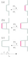
Three models of conformational switching. (a) Gating binding site. The binding site switches between being a reflecting boundary to being a radiation boundary. (b) Gated access. A lid along the passageway to the binding site transiently opens and closes, allowing for and blocking the passage of the ligand. (c) Gating binding pocket. The binding site becomes reactive only when the ligand is behind the closed lid. Note that in each model the binding pocket has a cylindrical shape, and a slice along the cylindrical axis is shown. The x axis is along the cylindrical axis.

All the three models of conformational switching have a cylindrical inner region, with the binding site located at the bottom. The previous analytical results themselves were based on approximations. These generalize Eq. 2.19 to²⁰

$$G_{\mathrm{g}}\left(\mathbf{r}\right)\approx \frac{e^{-\beta U_{\mathrm{g}}\left(\mathbf{r}\right)}{g}_{\mathrm{g}}\left(x\right)}{\sigma \left(x\right)e^{-\beta V_{\mathrm{g}}\left(x\right)}},$$ (3.4)

for the inner region. As with Eq. 2.19, these approximations can be well justified and the resulting k_a is expected to be accurate. Here, we refer to these results as “exact.” The governing equations for the inner region become

$$\begin{array}{ccc}& & \nabla ·\left\{D\sigma \left(x\right)e^{-\beta V_{\mathrm{a}}\left(x\right)}\nabla \left[g_{\mathrm{a}}\left(x\right)/\sigma \left(x\right)e^{-\beta V_{\mathrm{a}}\left(x\right)}\right]\right\}\hfill \\ & & -{\omega }_{-}\left(x\right)g_{\mathrm{a}}\left(x\right)+{\omega }_{+}\left(x\right)g_{\mathrm{i}}\left(x\right)=0,\hfill \end{array}$$ (3.5a)

$$\begin{array}{ccc}& & \nabla ·\left\{D\sigma \left(x\right)e^{-\beta V_{\mathrm{i}}\left(x\right)}\nabla \left[g_{\mathrm{i}}\left(x\right)/\sigma \left(x\right)e^{-\beta V_{\mathrm{i}}\left(x\right)}\right]\right\}\hfill \\ & & +{\omega }_{-}\left(x\right)g_{\mathrm{a}}\left(x\right)-{\omega }_{+}\left(x\right)g_{\mathrm{i}}\left(x\right)=0,\hfill \end{array}$$ (3.5b)

where

$${\omega }_{+}\left(x\right)=\frac{{\int }_{\mathrm{cross}\mathrm{section}\mathrm{at}x}ds{\omega }_{+}\left(\mathbf{r}\right)e^{-\beta U_{\mathrm{i}}\left(\mathbf{r}\right)}}{\sigma \left(x\right)e^{-\beta V_{\mathrm{i}}\left(x\right)}},$$ (3.6a)

$${\omega }_{-}\left(x\right)=\frac{{\int }_{\mathrm{cross}\mathrm{section}\mathrm{at}x}ds{\omega }_{-}\left(\mathbf{r}\right)e^{-\beta U_{\mathrm{a}}\left(\mathbf{r}\right)}}{\sigma \left(x\right)e^{-\beta V_{\mathrm{a}}\left(x\right)}}.$$ (3.6b)

The new detailed balance relation is

$$\frac{{\omega }_{+}\left(x\right)}{{\omega }_{-}\left(x\right)}=\frac{{\omega }_{\infty +}}{{\omega }_{\infty -}}{e}^{-\beta [V_{\mathrm{a}}\left(x\right)-V_{\mathrm{i}}\left(x\right)]}.$$ (3.7)

Within each model, two types of conformational switching are considered. The first, referred to as indifferent switch, was studied in earlier work.^{17, 24} In this type, ligand diffusion and conformational switching are uncoupled everywhere, even in the inner region. The second, referred to as induced switch, was introduced recently to account for the fact that protein-ligand interactions in the binding pocket often favor the switching to the active confornation.^{16, 21, 23} The boundary conditions on the dividing surface that led to the “exact” k_a results²⁰ were derived by assuming uncoupled ligand diffusion and conformational switching in the outer region and an infinitesimal layer around the dividing surface. Continuity of $g_{\mathrm{g}}\left(x\right)/\sigma \left(x\right)e^{-\beta V_{\mathrm{g}}\left(x\right)}$ and the flux $\mathcal{J}{g}_{\mathrm{g}}\left(x\right)\equiv D\sigma \left(x\right)e^{-\beta V_{\mathrm{g}}\left(x\right)}\nabla \left[g_{\mathrm{g}}\left(x\right)/\sigma \left(x\right)e^{-\beta V_{\mathrm{g}}\left(x\right)}\right]$ then took care of any transition to induced switch in the rest of the inner region.

Gating binding site

In this model (Fig. 2a), it is the binding site that switches between a reactive conformation and a non-reactive conformation. The former allows for ligand binding, with the binding site (at x = x_b) serving as a radiation boundary

$$\mathcal{J}{g}_{\mathrm{a}}\left(x_{\mathrm{b}}\right)={\kappa }_0{g}_{\mathrm{a}}\left(x_{\mathrm{b}}\right).$$ (3.8a)

In the latter conformation, the binding site is a reflecting boundary

$$\mathcal{J}{g}_{\mathrm{i}}\left(x_{\mathrm{b}}\right)=0.$$ (3.8b)

The boundary condition on the dividing surface (i.e., x = x_d), based on Eq. 3.4 and assuming uncoupled ligand diffusion and conformational switching in the outer region and an infinitesimal layer around the dividing surface, is²⁰

$$\mathcal{J}g\left(x_{\mathrm{d}}\right)=k_{\mathrm{E}}\left[1-\frac{g\left(x_{\mathrm{d}}\right)}{\sigma \left(x_{\mathrm{d}}\right)e^{-\beta V\left(x_{\mathrm{d}}\right)}}\right],$$ (3.9a)

$$\mathcal{J}f\left(x_{\mathrm{d}}\right)=-\omega {\widehat{k}}_{\mathrm{E}}\left(\omega \right)\frac{f\left(x_{\mathrm{d}}\right)}{\sigma \left(x_{\mathrm{d}}\right)e^{-\beta V\left(x_{\mathrm{d}}\right)}}.$$ (3.9b)

Here, g(x) and f(x), defined for x in an infinitesimal interval centered at x_d, are linear combinations of g_a(x) and g_i(x)

$$g\left(x\right)=g_{\mathrm{a}}\left(x\right)+g_{\mathrm{i}}\left(x\right),$$ (3.10a)

$$f\left(x\right)=p_{\mathrm{i}}{g}_{\mathrm{a}}\left(x\right)-p_{\mathrm{a}}{g}_{\mathrm{i}}\left(x\right),$$ (3.10b)

and ${\widehat{k}}_{\mathrm{E}}\left(s\right)$ is the Laplace transform of the time-dependent rate coefficient of the exterior problem [the steady-state value $k_{\mathrm{E}}=\underset{s\to 0}{lim}s{\widehat{k}}_{\mathrm{E}}\left(s\right)$].

BDflex gives a different boundary condition on the dividing surface. According to Eq. 2.22, this is

$${\left.-\frac{d{\eta }_{\mathrm{g}}\left(x\right)}{dx}\right|}_{x=x_{\mathrm{d}}}=\frac{k_{\mathrm{E}}}{\sigma \left(x_{\mathrm{d}}\right)e^{-\beta V\left(x_{\mathrm{d}}\right)}}{\eta }_{\mathrm{g}}\left(x_{\mathrm{d}}\right),$$ (3.11)

where the capture probability η_g(x) is related to the pair distribution function η_g(x) via

$$g_{\mathrm{g}}\left(x\right)=p_{\mathrm{g}}\sigma \left(x\right)e^{-\beta V_{\mathrm{g}}\left(x\right)}[1-{\eta }_{\mathrm{g}}\left(x\right)].$$ (3.12)

Note that the capture probabilities (or, equivalently, the pair distribution functions) for the two conformational states are uncoupled in Eq. 3.11, but coupled in Eqs. 3.9. The uncoupling offers a significant practical advantage in treating the boundary condition during BD simulations (see Sec. 4). The boundary condition of Eqs. 3.9 would be very cumbersome to implement in BD simulations.The boundary condition of Eq. 3.11 nevertheless is closely related to that of Eqs. 3.9. To see this, we express Eq. 3.11 in terms of the pair distribution functions

$$\mathcal{J}{g}_{\mathrm{g}}\left(x_{\mathrm{d}}\right)=k_{\mathrm{E}}\left[p_{\mathrm{g}}-\frac{g_{\mathrm{g}}\left(x_{\mathrm{d}}\right)}{\sigma \left(x_{\mathrm{d}}\right)e^{-\beta V\left(x_{\mathrm{d}}\right)}}\right].$$ (3.13a)

Using the combinations of Eq. 3.10, we further transform the boundary condition to

$$\mathcal{J}g\left(x_{\mathrm{d}}\right)=k_{\mathrm{E}}\left[1-\frac{g\left(x_{\mathrm{d}}\right)}{\sigma \left(x_{\mathrm{d}}\right)e^{-\beta V\left(x_{\mathrm{d}}\right)}}\right],$$ (3.13b)

$$\mathcal{J}f\left(x_{\mathrm{d}}\right)=-k_{\mathrm{E}}\frac{f\left(x_{\mathrm{d}}\right)}{\sigma \left(x_{\mathrm{d}}\right)e^{-\beta V\left(x_{\mathrm{d}}\right)}}.$$ (3.13c)

We now see that the BDflex boundary condition involves the further approximation of replacing $\omega {\widehat{k}}_{\mathrm{E}}\left(\omega \right)$ by k_E in the boundary condition for the function f(x). This replacement is strictly valid only in the limit of slow conformational transition (i.e., ω → 0). However, in the limit of fast conformational transition (i.e., ω → ∞), equilibration between the conformational states makes f(x) → 0, and the rate constant is then solely determined by g(x). Therefore, the BDflex boundary condition is correct in both the slow and fast limits of conformational transition, and is expected to be accurate overall. This expectation is confirmed by the results below.

Under indifferent switch, with a constant potential V₁ for both conformational states in the inner region having constant cross section σ, the rate constant calculated based on the boundary condition of Eqs. 3.9 is²⁰

$$\begin{array}{ccc}\hfill \frac{1}{k_{\mathrm{a}}}& =& \frac{1}{k_{\mathrm{E}}}+\frac{1}{p_{\mathrm{a}}{\kappa }_0\sigma e^{-\beta V_1}}+\frac{L_1}{D\sigma e^{-\beta V_1}}\hfill \\ & & +\frac{p_{\mathrm{i}}}{p_{\mathrm{a}}}\frac{\nu \coth \left(\nu L_1\right)+\omega {\widehat{k}}_{\mathrm{E}}\left(\omega \right)/D\sigma e^{-\beta V_1}}{\omega {\widehat{k}}_{\mathrm{E}}\left(\omega \right)\nu \coth \left(\nu L_1\right)+\omega \sigma e^{-\beta V_1}},\hfill \end{array}$$ (3.14)

where L₁ = x_d − x_b and ν = (ω/D)^1/2. In Subsection 3B, we will use k_GBS(L₁) to denote this rate constant, for binding to a gating binding site separated by a distance L₁ from the dividing surface. As noted above, the BDflex result involves replacing $\omega {\widehat{k}}_{\mathrm{E}}\left(\omega \right)$ by k_E

$$\begin{array}{ccc}\hfill \frac{1}{k_{\mathrm{a}}}& \approx & \frac{1}{k_{\mathrm{E}}}+\frac{1}{p_{\mathrm{a}}{\kappa }_0\sigma e^{-\beta V_1}}+\frac{L_1}{D\sigma e^{-\beta V_1}}\hfill \\ & & +\frac{p_{\mathrm{i}}}{p_{\mathrm{a}}}\frac{\nu \coth \left(\nu L_1\right)+k_{\mathrm{E}}/D\sigma e^{-\beta V_1}}{k_{\mathrm{E}}\nu \coth \left(\nu L_1\right)+\omega \sigma e^{-\beta V_1}},\hfill \end{array}$$ (3.15)

When ω → 0, both Eqs. 3.14, 3.15 predict

$$\begin{array}{c}\hfill \frac{1}{k_{\mathrm{a}}}\to \frac{1}{p_{\mathrm{a}}}\left(\frac{1}{k_{\mathrm{E}}}+\frac{1}{{\kappa }_0\sigma e^{-\beta V_1}}+\frac{L_1}{D\sigma e^{-\beta V_1}}\right),\end{array}$$ (3.16a)

which gives k_a as the product of the rate constant when the binding site stays reactive and the equilibrium probability for the reactive state. In the opposite limit ω → ∞, both

Eqs. 3.14, 3.15 predict

$$\frac{1}{k_{\mathrm{a}}}\to \frac{1}{k_{\mathrm{E}}}+\frac{1}{p_{\mathrm{a}}{\kappa }_0\sigma e^{-\beta V_1}}+\frac{L_1}{D\sigma e^{-\beta V_1}},$$ (3.16b)

which gives k_a as the rate constant when the binding site stays reactive but has reactivity p_aκ₀. Figure 3 shows that the BDflex result for k_a agrees with the “exact” result over the entire range of conformational transition rates. BDflex does break down when L₁ → 0; for the set of parameters chosen the discrepancy becomes noticeable at L₁/a = 0.1 (a: radius of the circular cross section of the inner region). So in implementing BDflex the dividing surface should be separated from the gating binding site by at least a small buffer region.

Figure 3.

Comparison of BDflex and “exact” results for the gating binding-site model. Curves represent the “exact” results and symbols represent the BDflex results. Results for two values of the distance, L₁, between the binding site and the dividing surface are shown. k_E = 4Da and κ₀ = ∞. For induced switch, ω₊/ω₋ = 0.01, ω_I+/ω_I− = 10, ω_I− = ω₋, and V_i = 0. Correspondingly, e^−βVeff = 11/1.01. For indifferent switch, ω₊/ω₋ = 0.01 and V₁ = V_eff.

Under induced switch, with a constant potential V_g for conformational state g and transition rates ω_I± between the states while the ligand is in the inner region, the rate constant calculated based on the boundary condition of Eqs. 3.9 is²⁰

$$\begin{array}{ccc}\hfill \frac{1}{k_{\mathrm{a}}}& =& \frac{1}{k_{\mathrm{E}}}+\frac{1}{p_{\mathrm{Ia}}{\kappa }_0\sigma e^{-\beta V_{e\mathrm{ff}}}}+\frac{L_1}{D\sigma e^{-\beta V_{e\mathrm{ff}}}}\hfill \\ & & {\displaystyle +\frac{p_{\mathrm{Ii}}}{p_{\mathrm{Ia}}}\frac{{\displaystyle \left({\displaystyle 1+\frac{\Delta p^2}{p_{\mathrm{Ii}}^2}}\right){\nu }_{\mathrm{I}}\coth \left({\nu }_{\mathrm{I}}{L}_1\right)+\frac{p_{\mathrm{a}}{p}_{\mathrm{i}}}{p_{\mathrm{Ia}}{p}_{\mathrm{Ii}}}\frac{\omega {\widehat{k}}_{\mathrm{E}}\left(\omega \right)}{D\sigma e^{-\beta V_{\mathrm{eff}}}}+\frac{2\Delta p}{p_{\mathrm{Ii}}}\frac{{\nu }_{\mathrm{I}}}{\sinh \left({\nu }_{\mathrm{I}}{L}_1\right)}}}{(p_{\mathrm{a}}{p}_{\mathrm{i}}/p_{\mathrm{Ia}}{p}_{\mathrm{Ii}})\omega {\widehat{k}}_{\mathrm{E}}\left(\omega \right){\nu }_{\mathrm{I}}\coth \left({\nu }_{\mathrm{I}}{L}_1\right)+{\omega }_{\mathrm{I}}\sigma e^{-\beta V_{\mathrm{eff}}}},}\hfill \end{array}$$ (3.17)

where ω_I = ω_I+ + ω_I−, p_Ia = ω_I+/ω_I, p_Ii = ω_I−/ω_I, Δp = p_Ia−p_a, ν_I = (ω_I/D)^1/2, and

$$e^{-\beta V\mathrm{eff}}=p_{\mathrm{a}}{e}^{-\beta V_{\mathrm{a}}}+p_{\mathrm{i}}{e}^{-\beta V_{\mathrm{i}}}.$$ (3.18)

Again the BDflex result is obtained by replacing $\omega {\widehat{k}}_{\mathrm{E}}\left(\omega \right)$ with k_E

$$\begin{array}{ccc}\hfill \frac{1}{k_{\mathrm{a}}}& =& \frac{1}{k_{\mathrm{E}}}+\frac{1}{p_{\mathrm{Ia}}{\kappa }_0\sigma e^{-\beta V_{e\mathrm{ff}}}}+\frac{L_1}{D\sigma e^{-\beta V_{e\mathrm{ff}}}}\hfill \\ & & {\displaystyle +\frac{p_{\mathrm{Ii}}}{p_{\mathrm{Ia}}}\frac{{\displaystyle \left({\displaystyle 1+\frac{\Delta p^2}{p_{\mathrm{Ii}}^2}}\right){\nu }_{\mathrm{I}}\coth \left({\nu }_{\mathrm{I}}{L}_1\right)+\frac{p_{\mathrm{a}}{p}_{\mathrm{i}}}{p_{\mathrm{Ia}}{p}_{\mathrm{Ii}}}\frac{k_{\mathrm{E}}}{D\sigma e^{-\beta V_{\mathrm{eff}}}}+\frac{2\Delta p}{p_{\mathrm{Ii}}}\frac{{\nu }_{\mathrm{I}}}{\sinh \left({\nu }_{\mathrm{I}}{L}_1\right)}}}{(p_{\mathrm{a}}{p}_{\mathrm{i}}/p_{\mathrm{Ia}}{p}_{\mathrm{Ii}})k_{\mathrm{E}}{\nu }_{\mathrm{I}}\coth \left({\nu }_{\mathrm{I}}{L}_1\right)+{\omega }_{\mathrm{I}}\sigma e^{-\beta V_{\mathrm{eff}}}}.}\hfill \end{array}$$ (3.19)

When ω → 0, both Eqs. 3.17, 3.19 predict

$$\frac{1}{k_{\mathrm{a}}}\to \frac{1}{p_{\mathrm{a}}}\left(\frac{1}{k_{\mathrm{E}}}+\frac{1}{{\kappa }_0\sigma e^{-\beta V_{\mathrm{a}}}}+\frac{L_1}{D\sigma e^{-\beta V_{\mathrm{a}}}}\right),$$ (3.20a)

which gives k_a as the product of the rate constant when the binding site stays reactive and the equilibrium probability for the reactive state. In the opposite limit ω → ∞, both Eqs. 3.17, 3.19 predict

$$\frac{1}{k_{\mathrm{a}}}\to \frac{1}{k_{\mathrm{E}}}+\frac{1}{p_{\mathrm{Ia}}{\kappa }_0\sigma e^{-\beta V_{e\mathrm{ff}}}}+\frac{L_1}{D\sigma e^{-\beta V_{e\mathrm{ff}}}},$$ (3.20b)

which gives k_a as the rate constant when the binding site stays active but has reactivity p_Iaκ₀ and the interaction potential is V_eff. As noted previously,^{16, 20, 21} relative to indifferent switch, the rate constant under induced switch has a reduced difference between the slow and fast limits of conformational transition, and the shift from the slow limit to the fast limit occurs at a lower conformational transition rate. Both effects serve to make the BDflex result more accurate over intermediate conformational transition rates. Figure 3 shows that the BDflex result for k_a agrees with the “exact” result over the entire range of conformational transition rates, even at L₁/a = 0.1.

Gated access

In the second model of conformational switching, a lid stochastically opens and closes the entrance to the binding site (Fig. 2b). The active and inactive conformations correspond to the open and closed lid, respectively. The boundary condition for g_a(x) at the location of the lid (where x = x₁), based on Eq. 3.4 and assuming that ligand diffusion and conformational switching are uncoupled all the way to an infinitesimal layer beyond x = x₁, is²⁰

$$\mathcal{J}{g}_{\mathrm{a}}\left(x_1\right)=k_{\mathrm{GBS}}\left(L_1\right)\left(1-\frac{g_{\mathrm{a}}\left(x_1\right)}{p_{\mathrm{a}}\sigma \left(x_1\right)e^{-\beta V\left(x_1\right)}}\right),$$ (3.21a)

where k_GBS(L₁) is the rate constant for binding to a gating binding site, with κ₀ = ∞, located at a distance L₁ = x_d − x₁ from the dividing surface [see Eq. 3.14]. For g_i(x) the boundary condition at x = x₁ is reflecting

$$\mathcal{J}{g}_{\mathrm{i}}\left(x_1\right)=0.$$ (3.21b)

The binding site serves as a radiation boundary for both g_a(x) and g_i(x)

$$\mathcal{J}{g}_{\mathrm{a}}\left(x_{\mathrm{b}}\right)={\kappa }_0{g}_{\mathrm{a}}\left(x_{\mathrm{b}}\right),$$ (3.22a)

$$\mathcal{J}{g}_{\mathrm{i}}\left(x_{\mathrm{b}}\right)={\kappa }_0{g}_{\mathrm{i}}\left(x_{\mathrm{b}}\right).$$ (3.22b)

Under indifferent switch, with a constant potential V₀ for both conformational states when the ligand is in the binding pocket (i.e., x_b ≤ x ≤ x₁), the rate constant calculated based on the boundary condition of Eqs. 3.21 is²⁰

$$\begin{array}{ccc}\hfill \frac{1}{k_{\mathrm{a}}}& =& \frac{1}{k_{\mathrm{GBS}}\left(L_1\right)}+\frac{1}{{\kappa }_0\sigma e^{-\beta V_0}}+\frac{L}{D\sigma e^{-\beta V_0}}\hfill \\ & & +\frac{p_{\mathrm{i}}}{p_{\mathrm{a}}}\frac{\nu \coth \left(\nu L\right)+k_0/D\sigma e^{-\beta V_0}}{k_0\nu \coth \left(\nu L\right)+\omega \sigma e^{-\beta V_0}},\hfill \end{array}$$ (3.23a)

where L = x₁ − x_b and $k_0={\kappa }_0\sigma e^{-\beta V_0}$. Note the resemblance of Eq. 3.15 to Eq. 3.23a. In the former problem, the reactivity stays at $k_{\mathrm{E}}/\sigma e^{-\beta V_1}$ at one end of the binding pocket and switches between κ₀ and 0 at the other end [see Eqs. 3.13a, 3.8, respectively]; in the latter problem, the reactivity stays at κ₀ at one end of the binding pocket and switches between $k_{\mathrm{GBS}}\left(L_1\right)/p_{\mathrm{a}}\sigma e^{-\beta V_0}$ and 0 at the other end [see Eqs. 3.22, 3.21, respectively]. If the potential takes a constant value V₁ for x₁ ≤ x ≤ x_d, then k_GBS(L₁) is given by Eq. 3.14 with κ₀ = ∞. Consequently,

$$\begin{array}{ccc}\hfill \frac{1}{k_{\mathrm{a}}}& =& \frac{1}{k_{\mathrm{E}}}+\frac{L_1}{D\sigma e^{-\beta V_1}}+\frac{1}{{\kappa }_0\sigma e^{-\beta V_0}}+\frac{L}{D\sigma e^{-\beta V_0}}\hfill \\ & & +\frac{p_{\mathrm{i}}}{p_{\mathrm{a}}}\frac{\nu \coth \left(\nu L_1\right)+\omega {\widehat{k}}_{\mathrm{E}}\left(\omega \right)/D\sigma e^{-\beta V_1}}{\omega {\widehat{k}}_{\mathrm{E}}\left(\omega \right)\nu \coth \left(\nu L_1\right)+\omega \sigma e^{-\beta V_1}}\hfill \\ & & +\frac{p_{\mathrm{i}}}{p_{\mathrm{a}}}\frac{\nu \coth \left(\nu L\right)+k_0/D\sigma e^{-\beta V_0}}{k_0\nu \coth \left(\nu L\right)+\omega \sigma e^{-\beta V_0}}.\hfill \end{array}$$ (3.23b)

This result could have been derived by using: (1) the boundary condition of Eqs. 3.9 at x = x_d; (2) the continuity conditions for $g_{\mathrm{a}}\left(x\right)e^{\beta V_{\mathrm{a}}\left(x\right)}$ and $\mathcal{J}{g}_{\mathrm{a}}\left(x\right)$ and reflecting boundary condition for g_i(x) at x = x₁; and (3) the radiation boundary conditions for g_a(x) and g_i(x) at x = x_b.

We now present the rate constant calculated according to BDflex. This would use the three sets of conditions just listed, except that Eqs. 3.9 at x = x_d are replaced by Eqs. 3.13b, 3.13c. More specifically, $\omega {\widehat{k}}_{\mathrm{E}}\left(\omega \right)$ is replaced by k_E. Therefore, the BDflex result is

$$\begin{array}{ccc}\hfill \frac{1}{k_{\mathrm{a}}}& =& \frac{1}{k_{\mathrm{E}}}+\frac{L_1}{D\sigma e^{-\beta V_1}}+\frac{1}{{\kappa }_0\sigma e^{-\beta V_0}}+\frac{L}{D\sigma e^{-\beta V_0}}\hfill \\ & & +\frac{p_{\mathrm{i}}}{p_{\mathrm{a}}}\frac{\nu \coth \left(\nu L_1\right)+k_{\mathrm{E}}/D\sigma e^{-\beta V_1}}{k_{\mathrm{E}}\nu \coth \left(\nu L_1\right)+\omega \sigma e^{-\beta V_1}}\hfill \\ & & +\frac{p_{\mathrm{i}}}{p_{\mathrm{a}}}\frac{\nu \coth \left(\nu L\right)+k_0/D\sigma e^{-\beta V_0}}{k_0\nu \coth \left(\nu L\right)+\omega \sigma e^{-\beta V_0}}.\hfill \end{array}$$ (3.24)

When ω → ∞, both Eqs. 3.23b, 3.24 predict

$$\begin{array}{c}\hfill \frac{1}{k_{\mathrm{a}}}\to \frac{1}{k_{\mathrm{E}}}+\frac{L_1}{D\sigma e^{-\beta V_1}}+\frac{1}{{\kappa }_0\sigma e^{-\beta V_0}}+\frac{L}{D\sigma e^{-\beta V_0}},\end{array}$$ (3.25a)

which gives k_a as the rate constant when the lid stays open. In the opposite limit ω → 0, both Eqs. 3.23b, 3.24 predict

$$\begin{array}{c}\hfill \frac{1}{k_{\mathrm{a}}}\to \frac{1}{p_{\mathrm{a}}}\left(\frac{1}{k_{\mathrm{E}}}+\frac{L_1}{D\sigma e^{-\beta V_1}}+\frac{1}{{\kappa }_0\sigma e^{-\beta V_0}}+\frac{L}{D\sigma e^{-\beta V_0}}\right),\end{array}$$ (3.25b)

which gives k_a as the product of the rate constant when the lid stays open and the equilibrium probability for the lid being open. Figure 4 shows the good agreement between the BDflex “exact” results over the entire range of conformational transition rates. BDflex still breaks down when L₁ → 0 (not shown); so again the dividing surface should be separated by a buffer from the region (the lid in the present case) undergoing conformational transition to ensure accuracy of BDflex.

Figure 4.

Comparison of BDflex and “exact” results for the gated access model. L₁/a = 1 and L/a = 5, where L₁ is the distance between the lid and the dividing surface and L is the distance between the binding site and the lid. k_E = 4Da and κ₀ = 0.01D/a. The gating parameters for induced switch are the same as in Fig. 3; in addition V₁ = V_eff. For indifferent switch, ω₊/ω₋ = 0.01 and V₀ = V₁ = V_eff.

Next we consider induced switch, with a constant potential V_g for conformational state g and transition rates ω_I± between the states when the ligand is in the binding pocket. The interaction of the ligand with the binding pocket favors the lid open state (i.e., p_Ia/p_Ii ≫ p_a/p_i). The problem can again be solved by using the three sets of conditions at x = x_d, x₁, and x_b. The “exact” result for k_a is given by

$$\begin{array}{ccc}\hfill \frac{1}{k_{\mathrm{a}}}& =& \frac{1}{k_{\mathrm{E}}}+\frac{L_1}{D\sigma e^{-\beta V_1}}+\frac{1}{{\kappa }_0\sigma e^{-\beta V_{\mathrm{eff}}}}+\frac{L}{D\sigma e^{-\beta V_{\mathrm{eff}}}}\hfill \\ & & +\frac{p_{\mathrm{i}}}{p_{\mathrm{a}}}\frac{\nu \coth \left(\nu L_1\right)+\omega {\widehat{k}}_{\mathrm{E}}\left(\omega \right)/D\sigma e^{-\beta V_1}}{\omega {\widehat{k}}_{\mathrm{E}}\left(\omega \right)\nu \coth \left(\nu L_1\right)+\omega \sigma e^{-\beta V_1}}\hfill \\ & & +\frac{p_{\mathrm{Ii}}}{p_{\mathrm{Ia}}}\frac{{\nu }_{\mathrm{I}}\coth \left({\nu }_{\mathrm{I}}L\right)+{\kappa }_0/D}{{\kappa }_0\sigma e^{-\beta V_{\mathrm{eff}}}{\nu }_{\mathrm{I}}\coth \left({\nu }_{\mathrm{I}}L\right)+{\omega }_{\mathrm{I}}\sigma e^{-\beta V_{\mathrm{eff}}}}.\hfill \end{array}$$ (3.26)

This is nearly identical to Eq. 3.23b, except that here V_eff, p_Ia, and p_Ii in the binding pocket substitute for V₀, p_a, and p_i, respectively. The BDflex result is obtained by replacing $\omega {\widehat{k}}_{\mathrm{E}}\left(\omega \right)$ with k_E in Eq. 3.26

$$\begin{array}{ccc}\hfill \frac{1}{k_{\mathrm{a}}}& =& \frac{1}{k_{\mathrm{E}}}+\frac{L_1}{D\sigma e^{-\beta V_1}}+\frac{1}{{\kappa }_0\sigma e^{-\beta V_{\mathrm{eff}}}}+\frac{L}{D\sigma e^{-\beta V_{\mathrm{eff}}}}\hfill \\ & & +\frac{p_{\mathrm{i}}}{p_{\mathrm{a}}}\frac{\nu \coth \left(\nu L_1\right)+k_{\mathrm{E}}/D\sigma e^{-\beta V_1}}{k_{\mathrm{E}}\nu \coth \left(\nu L_1\right)+\omega \sigma e^{-\beta V_1}}\hfill \\ & & +\frac{p_{\mathrm{Ii}}}{p_{\mathrm{Ia}}}\frac{{\nu }_{\mathrm{I}}\coth \left({\nu }_{\mathrm{I}}L\right)+{\kappa }_0/D}{{\kappa }_0\sigma e^{-\beta V_{\mathrm{eff}}}{\nu }_{\mathrm{I}}\coth \left({\nu }_{\mathrm{I}}L\right)+{\omega }_{\mathrm{I}}\sigma e^{-\beta V_{\mathrm{eff}}}}.\hfill \end{array}$$ (3.27)

When ω → 0, both Eqs. 3.26, 3.27 predict

$$\begin{array}{c}\hfill \frac{1}{k_{\mathrm{a}}}\to \frac{1}{p_{\mathrm{a}}}\left(\frac{1}{k_{\mathrm{E}}}+\frac{L_1}{D\sigma e^{-\beta V_1}}+\frac{1}{{\kappa }_0\sigma e^{-\beta V_{\mathrm{a}}}}+\frac{L}{D\sigma e^{-\beta V_{\mathrm{a}}}}\right),\end{array}$$ (3.28a)

which gives k_a as the product of the rate constant when the lid stays open (with the potential being V₁ for x₁ < x < x_d and V_a for x_b < x < x₁) and the equilibrium probability for the lid being open. In the opposite limit ω → ∞, both Eqs. 3.26, 3.27 predict

$$\begin{array}{c}\hfill \frac{1}{k_{\mathrm{a}}}\to \frac{1}{k_{\mathrm{E}}}+\frac{L_1}{D\sigma e^{-\beta V_1}}+\frac{1}{{\kappa }_0\sigma e^{-\beta V_{\mathrm{eff}}}}+\frac{L}{D\sigma e^{-\beta V_{\mathrm{eff}}}},\end{array}$$ (3.28b)

which gives k_a as the rate constant when the lid stays open, with the potential being V₁ for x₁ < x < x_d and V_eff for x_b < x < x₁. Figure 4 shows the good agreement between the BDflex and exact results for k_a in the gated access case under induced switch. Also note that, similar to the gating binding-site case, induced switch has the advantage over indifferent switch in that the rate constant has a reduced difference between the slow and fast limits of conformational transition and the shift from the slow limit to the fast limit occurs at a lower conformational transition rate.

Gating binding pocket

The third model of conformational switching also has a lid at the entrance to the binding pocket, but after the ligand is inside, the lid must be closed for the binding site to be reactive (Fig. 2c). The active conformation of the binding pocket has the lid closed and the binding site reactive, whereas the inactive conformation of the binding pocket has the lid open and the binding site non-reactive.²⁵ The boundary conditions at the binding site become

$$\mathcal{J}{g}_{\mathrm{a}}\left(x_{\mathrm{b}}\right)={\kappa }_0{g}_{\mathrm{a}}\left(x_{\mathrm{b}}\right),$$ (3.29a)

$$\mathcal{J}{g}_{\mathrm{i}}\left(x_{\mathrm{b}}\right)=0.$$ (3.29b)

Like the gated access case, the problem can be solved by using three sets of conditions at x = x_d, x₁, and x_b. At x = x_d, the “exact” boundary condition is given by Eqs. 3.9. At x = x₁, g_a(x) encounters a reflecting boundary but $g_{\mathrm{i}}\left(x\right)e^{\beta V_{\mathrm{i}}\left(x\right)}$ and $\mathcal{J}{g}_{\mathrm{i}}\left(x\right)$ are continuous. At x = x_b, the boundary conditions for g_a(x) and g_i(x) are given by Eqs. 3.29.

Under indifferent switch, with transition rates ω_± between the inactive and active conformations regardless of where the ligand is, the “exact” rate constant is given by

$$\begin{array}{ccc}\hfill \frac{1}{k_{\mathrm{a}}}& =& \frac{1}{k_{\mathrm{E}}}+\frac{L_1}{D\sigma e^{-\beta V_1}}+\frac{1}{p_{\mathrm{a}}{\kappa }_0\sigma e^{-\beta V_0}}+\frac{L}{D\sigma e^{-\beta V_0}}\hfill \\ & & +\frac{p_{\mathrm{a}}}{p_{\mathrm{i}}}\frac{\nu \coth \left(\nu L_1\right)+\omega {\widehat{k}}_{\mathrm{E}}\left(\omega \right)/D\sigma e^{-\beta V_1}}{\omega {\widehat{k}}_{\mathrm{E}}\left(\omega \right)\nu \coth \left(\nu L_1\right)+\omega \sigma e^{-\beta V_1}}\hfill \\ & & +\left(\frac{p_{\mathrm{i}}}{p_{\mathrm{a}}}+\frac{p_{\mathrm{a}}}{p_{\mathrm{i}}}\right)\frac{\nu \coth \left(\nu L\right)}{\omega \sigma e^{-\beta V_0}}+\frac{2\nu }{\omega \sigma e^{-\beta V_0}\sinh \left(\nu L\right)}.\hfill \end{array}$$ (3.30)

The BDflex result is obtained by replacing $\omega {\widehat{k}}_{\mathrm{E}}\left(\omega \right)$ with k_E

$$\begin{array}{ccc}\hfill \frac{1}{k_{\mathrm{a}}}& =& \frac{1}{k_{\mathrm{E}}}+\frac{L_1}{D\sigma e^{-\beta V_1}}+\frac{1}{p_{\mathrm{a}}{\kappa }_0\sigma e^{-\beta V_0}}+\frac{L}{D\sigma e^{-\beta V_0}}\hfill \\ & & +\frac{p_{\mathrm{a}}}{p_{\mathrm{i}}}\frac{\nu \coth \left(\nu L_1\right)+k_{\mathrm{E}}/D\sigma e^{-\beta V_1}}{k_{\mathrm{E}}\nu \coth \left(\nu L_1\right)+\omega \sigma e^{-\beta V_1}}\hfill \\ & & +\left(\frac{p_{\mathrm{i}}}{p_{\mathrm{a}}}+\frac{p_{\mathrm{a}}}{p_{\mathrm{i}}}\right)\frac{\nu \coth \left(\nu L\right)}{\omega \sigma e^{-\beta V_0}}+\frac{2\nu }{\omega \sigma e^{-\beta V_0}\sinh \left(\nu L\right)}.\hfill \end{array}$$ (3.31)

When ω → 0, both Eqs. 3.26, 3.27 predict k_a → 0. The fast-transition limit is

$$\begin{array}{c}\hfill \frac{1}{k_{\mathrm{a}}}\to \frac{1}{k_{\mathrm{E}}}+\frac{L_1}{D\sigma e^{-\beta V_1}}+\frac{1}{p_{\mathrm{a}}{\kappa }_0\sigma e^{-\beta V_0}}+\frac{L}{D\sigma e^{-\beta V_0}}.\end{array}$$ (3.32)

The results under induced switch can be obtained by substituting V_eff, p_Ia, and p_Ii in the binding pocket for V₀, p_a, and p_i, respectively. The “exact” result for k_a is given by

$$\begin{array}{ccc}\hfill \frac{1}{k_{\mathrm{a}}}& =& \frac{1}{k_{\mathrm{E}}}+\frac{L_1}{D\sigma e^{-\beta V_1}}+\frac{1}{p_{\mathrm{Ia}}{\kappa }_0\sigma e^{-\beta V_{\mathrm{eff}}}}+\frac{L}{D\sigma e^{-\beta V_{\mathrm{eff}}}}\hfill \\ & & +\frac{p_{\mathrm{a}}}{p_{\mathrm{i}}}\frac{\nu \coth \left(\nu L_1\right)+\omega {\widehat{k}}_{\mathrm{E}}\left(\omega \right)/D\sigma e^{-\beta V_1}}{\omega {\widehat{k}}_{\mathrm{E}}\left(\omega \right)\nu \coth \left(\nu L_1\right)+\omega \sigma e^{-\beta V_1}}\hfill \\ & & +\left(\frac{p_{\mathrm{Ii}}}{p_{\mathrm{Ia}}}+\frac{p_{\mathrm{Ia}}}{p_{\mathrm{Ii}}}\right)\frac{{\nu }_{\mathrm{I}}\coth \left({\nu }_{\mathrm{I}}L\right)}{{\omega }_{\mathrm{I}}\sigma e^{-\beta V_{\mathrm{eff}}}}+\frac{2{\nu }_{\mathrm{I}}}{{\omega }_{\mathrm{I}}\sigma e^{-\beta V_{\mathrm{eff}}}\sinh \left({\nu }_{\mathrm{I}}L\right)}.\hfill \end{array}$$ (3.33)

The BDflex result is

$$\begin{array}{ccc}\hfill \frac{1}{k_{\mathrm{a}}}& =& \frac{1}{k_{\mathrm{E}}}+\frac{L_1}{D\sigma e^{-\beta V_1}}+\frac{1}{p_{\mathrm{Ia}}{\kappa }_0\sigma e^{-\beta V_{\mathrm{eff}}}}+\frac{L}{D\sigma e^{-\beta V_{\mathrm{eff}}}}\hfill \\ & & +\frac{p_{\mathrm{a}}}{p_{\mathrm{i}}}\frac{\nu \coth \left(\nu L_1\right)+k_{\mathrm{E}}/D\sigma e^{-\beta V_1}}{k_{\mathrm{E}}\nu \coth \left(\nu L_1\right)+\omega \sigma e^{-\beta V_1}}\hfill \\ & & +\left(\frac{p_{\mathrm{Ii}}}{p_{\mathrm{Ia}}}+\frac{p_{\mathrm{Ia}}}{p_{\mathrm{Ii}}}\right)\frac{{\nu }_{\mathrm{I}}\coth \left({\nu }_{\mathrm{I}}L\right)}{{\omega }_{\mathrm{I}}\sigma e^{-\beta V_{\mathrm{eff}}}}+\frac{2{\nu }_{\mathrm{I}}}{{\omega }_{\mathrm{I}}\sigma e^{-\beta V_{\mathrm{eff}}}\sinh \left({\nu }_{\mathrm{I}}L\right)}.\hfill \end{array}$$ (3.34)

Figure 5 shows that, for both indifferent switch and induced switch, the BD results for k_a agree well with the exact results. Induced switch results in higher k_a and a shift to the fast limit of conformational transition at a lower transition rate.

Figure 5.

Comparison of BDflex and “exact” results for the gating binding-pocket model. The parameters are the same as in Fig. 4, except κ₀ = D/a.

IMPLEMENTATION OF BDflex

We now illustrate the implementation of BDflex on a model system, consisting of a spherical-shaped protein (radius R) with a buried binding pocket and a pointlike ligand (Fig. 1b). The binding pocket is defined by a second, smaller sphere, centered a distance d from the center of the protein sphere; the binding pocket includes only the portion of the second sphere that is inside the protein sphere. For convenience we define the center of the protein sphere as the origin of a coordinate system, and the center of the binding-pocket sphere as lying on the x axis. The ligand cannot penetrate the protein surface. Inside the binding pocket the ligand can bind to the protein with a rate constant γ. The protein either has a rigid structure or can undergo conformational switching. In the latter case, the radius of the binding pocket stochastically switches, with rates ω_±, between two values, a and a^′; binding can occur only when the binding pockets adopts the second size. Both indifferent switch and induced switch are studied. We implement both the 1990 algorithm³ for k_a calculation and BDflex to demonstrate the latter's considerable savings in computational time. All times reported below are in units of R²/2D, which has a typical value ∼2 ns.

Implementation procedure

We first summarize the 1990 algorithm. This is also the algorithm that we use to solve the exterior problem of BDflex. In addition, the implementation of the interior problem of BDflex shares many ingredients with the 1990 algorithm. In that algorithm, ligand trajectories are started in the reaction region and then propagated up to a cutoff time (t_cut). Whenever the ligand is inside the reaction region it is allowed to form the product (with rate constant γ). If production formation occurs, then the trajectory is terminated. The lifetime of that trajectory is recorded. If production formation does not occur before t_cut, then the lifetime of the trajectory is recorded as >t_cut. For these lifetimes, the fraction of surviving trajectories at times up to t_cut is calculated. The survival fraction, S(t), is related to the time-dependent rate coefficient k(t) via

$$k\left(t\right)=k\left(0\right)S\left(t\right).$$ (4.1)

The initial value of the rate coefficient is

$$k\left(0\right)=p_{\mathrm{a}}{V}_{\mathrm{rr}}{⟨e_{\mathrm{rr}}^{-\beta U_{\mathrm{a}}\left(\mathbf{r}\right)}⟩}_{\mathrm{rr}}\gamma ,$$ (4.2)

where V_rr is the volume of the reaction region. Note that in the case of the protein undergoing conformational switching, the reaction region is the binding pocket with radius a^′. The average Boltzmann factor is present if the protein-ligand interaction potential is not zero when the ligand is in the reaction region and the protein is in the reactive conformation. The long-time limit of k(t) is the rate constant k_a. This is obtained by fitting the long-time portion of k(t) to the known asymptotic expansion²⁶

$$k\left(t\right)=k_{\mathrm{a}}[1+k_{\mathrm{a}}/4\pi D{\left(\pi Dt\right)}^{1/2}+\cdots ].$$ (4.3)

To ensure conformity to the asymptotic behavior, t_cut has to be sufficiently large.

The 1990 algorithm works both when the protein has a rigid structure and when it undergoes conformational switching. However, the latter case may require enormous computational time, which is the motivation for the present work. For the model problem of Fig. 1b, this is not a problem and we can use the 1990 algorithm for benchmarking. Some details of the implementation here are as follows. The propagation of ligand trajectories follows the Ermak-McCammon algorithm.²⁷ The reflecting boundary condition on the protein surface is treated by placing the ligand back to its prior position. The timesteps are 10⁻⁵ when inside a sphere with radius R₁ = 1.1R and 10⁻⁵ + 10⁻²(r − R₁)²/2D otherwise. In the case of the protein undergoing conformational switching, when the binding pocket switches from the large size to the smaller size, the ligand could be found in a forbidden region. In that case the ligand is moved toward the center of binding pocket to just inside it.

The protein-ligand interaction potential is absent in the case of a rigid binding pocket and in the case of indifferent switch between an open (with radius a) but non-reactive conformation and a closed (with radius a^′) but reactive conformation. However, under induced switch, the ligand in the reaction region should interact favorably with the protein in the reactive conformation. We thus assign a negative value, U₀, to U_a(r) for r in the reactive region. Around r = R, the interaction potential makes a smooth but sharp transition to zero²¹

$$U_{\mathrm{a}}\left(\mathbf{r}\right)=-\frac{U_0}{2}(\tanh \frac{r-R}{L}-1).$$ (4.4)

We choose L/R = 0.005. The potential for the non-reactive conformation, U_i(r), is zero both in the binding pocket and in the outside.

BDflex consists of two sets of BD simulations, solving the exterior and interior problems, respectively. We use different choices of the dividing surface to check whether and how the calculated k_a depends on the choice of the dividing surface. The inner most choice is the mouth of the binding pocket (green solid curve in Fig. 1b); a choice that is slightly displaced outward is the exposed cap of the binding-pocket sphere (dashed curve in Fig. 1b); other choices include the exposed surface of a third sphere, with various radii and centered at various positions on the x axis, that intersects the protein sphere.

As already mentioned, the exterior simulations follow the 1990 algorithm to yield k_E; here the protein is treated as rigid. The boundary condition on the dividing surface should be absorbing. However, the 1990 algorithm cannot directly handle the absorbing boundary condition. Instead, we turn the boundary condition into the radiation type, and then let the reactivity κ approach infinity. Actually the 1990 algorithm cannot directly handle the radiation boundary either. The way out³ is to grow the dividing surface outward into a thin spherical shell, with thickness ɛ; the original dividing surface is turned into a reflecting boundary but the thin shell is turned into a reaction region. With a reaction rate equal to κ/ɛ, it can be shown that this treatment approximates the radiation boundary condition well when ɛ is small [see Eq. 2.33]. Note that now the outer region has its entire inner boundary, defined by the dividing surface plus the protein surface connected to it, satisfying the reflecting condition, which ensures that the ligand is restricted to the outer region. We use a similar treatment for implementing the radiation boundary condition, Eq. 2.22, of the interior problem (see below). Hereafter, we refer to the thin shell bordering the dividing surface as the sink region, to distinguish from the reaction region modeling ligand binding. With ligand trajectories started in the sink region and allowed to react with rate κ/ɛ, we obtain the rate constant k for a series of κ values. The desired k_E is obtained from fitting the dependence of k on κ according to²⁶

$$\frac{1}{k}=\frac{1}{V_{\mathrm{sr}}\kappa /\varepsilon }+\frac{1}{k_{\mathrm{E}}},$$ (4.5)

where V_sr is the volume of the sink region (an average Boltzmann factor would be present should the protein-ligand interaction potential be not zero in the sink region).

In the interior simulations, as mentioned above we transform the radiation boundary condition on the dividing surface [Eq. 2.22] into the sink region with reaction rate κ_E/ε, where κ_E = k_E/σ_d [see Eq. 2.18]. To confine the ligand to the inner region, we make the dividing surface invisible but the remaining surface of the sink region reflecting. Ligand trajectories are started in the sink region and are propagated until reaction occurs either in the sink region or in the reaction region. The fraction of trajectories that end up reacting in the reaction region is ${\overline{\eta }}_{\mathrm{d}}$. Finally, the product k_E${\overline{\eta }}_{\mathrm{d}}$ gives the overall rate constant k_a.

Note that the same radiation boundary condition, Eq. 2.22, is valid for any conformational state. Therefore, its implementation during the BD simulations is the same even in the presence of conformational fluctuations. A more rigorous formulation of the boundary condition would involve coupling of different conformational states [see, e.g., Eqs. 3.9]. That type of boundary condition would be far more cumbersome to implement.

In the 1990 algorithm, the ligand crosses the dividing surface multiple times before reaction at the binding site (or the trajectory is terminated by exceeding the t_cut threshold). By confining the ligand to the inner region and then imposing the radiation boundary condition, BDflex avoids such multiple-crossing of the dividing surface. This results in considerable savings in computational time, as shown below.

Results

In Fig. 6a, we compare k_a values obtained by the 1990 algorithm and by BDflex for a rigid binding pocket with a range γ, which is the rate of product formation inside the binding pocket. We implemented BDflex using two dividing surfaces (Fig. 1b), resulting in k_E = 1.01DR and 1.36DR, respectively. The final results for k_a are very similar and both are close to the results by the 1990 algorithm. Other dividing surfaces also give very similar results (not shown).

Figure 6.

Comparison of simulation results according to BDflex and to the 1990 algorithm. (a) Rigid binding pocket. a/R = 0.25; d/R = 0.86. (b) Binding pocket undergoing indifferent switch. The binding pocket switches between an open (with radius a) but non-reactive state and a closed (with radius a^′ = R−d = 0.14R) but reactive state, with ω₊ = ω₋ = 10D/R². The solid and dashed curves are BDflex results using two alternative dividing surfaces (Fig. 1b); symbols are results by the 1990 algorithm. For R²γ/D ≤ 10, the number of trajectories in the BDflex interior simulations is increased tenfold to 40 000, to demonstrate that long simulations for these more challenging cases can be afforded by BDflex. (c) Binding pocket undergoing induced switch. The rates of conformation switch are ω₊ = D/R² and ω₋ = 10D/R² when the ligand is far away but change to ω_I+ = 100D/R² and ω_I− = 10D/R² when the ligand is inside the binding pocket. Correspondingly, $e^{-\beta U_0}$ = 100. The solid curve displays BDflex results using the solid dividing surface in Fig. 1b; symbols are results by the 1990 algorithm.

Relative to k_a by the 1990 algorithm, ${\overline{\eta }}_{\mathrm{d}}$ converges with a smaller number of trajectories. The k_a values shown in Fig. 6a are obtained using 6000 trajectories each by the 1990 algorithm but using 4000 trajectories for BDflex. Moreover, the total simulation time per trajectory is significantly reduced in the BDflex simulations, except for very high γ, under which most of the trajectories in the 1990 algorithm terminate before they leave the reaction region. The factor by which the CPU time of the BDflex results over that by the 1990 algorithm is shown in Fig. 7. Threefold speedup is obtained.

Figure 7.

The ratio of CPU times of BDflex and the 1990 algorithm. In each of the three cases studied, CPU times are from a total of 4000 trajectories for BDflex and 6000 trajectories for the 1990 algorithm.

In Fig. 6b, we display k_a values for the binding pocket under indifferent switch, between an open but non-reactive conformation and a closed but reactive conformation (Fig. 1b), similar to the gating binding-pocket model of the preceding section. Again the BDflex results agree very well with results obtained by the 1990 algorithm. Relative to the rigid binding pocket, product formation in the present case becomes a rarer event; hence k_a is reduced in magnitude. Here, the saving in CPU time by BDflex becomes even more significant, with speedup as much as eightfold (Fig. 7). So BDflex becomes powerful especially for problems that are challenging to the traditional approaches.

In Fig. 6c, we display k_a values for the binding pocket under induced switch. Again the BDflex results agree very well with results obtained by the 1990 algorithm. Relative to the indifferent switch case, the magnitude of k_a is higher, suggesting that a protein can use adaption of its conformation to the incoming ligand to speed up the binding process. Here again there is a significant saving in CPU time by BDflex, with speedup of ∼5.5-fold (Fig. 7).

While we do not show explicit results for the saving in CPU time by BDflex over the 1984 algorithm of Northrup et al.,¹ a comparison of the algorithm designs makes it clear that BDflex should be significantly faster. In essence both algorithms find k_a by breaking it into the form k_a = k_Eη [see Eqs. 1.1, 2.15]. We choose a dividing surface that is as close to the binding pocket as possible, such that k_E approximates k_a as much as possible and, η, the probability for a ligand starting on the dividing surface to react in the binding pocket, instead of escape to infinity, is as high as possible. A higher η makes it easier and hence requires less number of trajectories to determine. In contrast, the Northrup et al. algorithm uses a spherical dividing surface, so k_E is generally much higher than k_a, and corresponding η is very small, especially when ligand binding is accompanied by protein conformational change, the case that motivated the present paper. The radiation boundary condition that we introduce here on the dividing surface so as to confine the motion of the ligand to the inner region may provide an additional saving in computational time.

CONCLUDING REMARKS

We have developed a new method, BDflex, for efficiently treating conformational fluctuations in calculating protein-ligand binding rate constants (k_a) from Brownian dynamics simulations. The core idea of BDflex, breaking up the calculation of k_a into separate exterior and interior problems, can be traced to theoretical developments over the years.^{16, 17, 19, 20} Connecting the exterior and interior problems is a critical link, and here we are able to treat this link via a radiation boundary condition that can be conveniently implemented in Brownian dynamics simulations, even in the presence of conformational fluctuations.

The radiation boundary condition on the dividing surface of the outer and inner regions is an approximation and we have demonstrated its accuracy on models of conformational fluctuations. Moreover, we have illustrated the implementation of BDflex on a model system and compared to the implementation of a previous algorithm³ for calculating k_a from BD simulations. The latter algorithm does not invoke any approximation. Here, we show that BDflex yields the same k_a values at considerably reduced computational cost. The ligand in the inner region can either react in the binding site or be absorbed on the dividing surface. The avoidance of crossing the dividing surface multiple times before binding to the protein accounts for the savings in computational time.

The implementation of BDflex illustrated here has demonstrated its accuracy and expected considerable savings in computational time. This implementation did not rely on anything specific to the chosen model system and can be easily ported to more realistic models of protein-ligand systems. In such models, proteins and ligands are represented with more molecular details, albeit still at a coarse-grained level for practical purposes. Such models, after careful parameterization, allow both overall translational and rotational diffusion and internal conformational fluctuations to be modeled by Brownian dynamics simulations.²⁸ Implementation of BDflex within such more realistic models of protein-ligand systems is underway.

References

- Northrup S. H., Allison S. A., and McCammon J. A., J. Chem. Phys. 80, 1517 (1984). 10.1063/1.446900 [DOI] [Google Scholar]
- Luty B. A., McCammon J. A., and Zhou H. X., J. Chem. Phys. 97, 5682 (1984). 10.1063/1.463777 [DOI] [Google Scholar]
- Zhou H.-X., J. Phys. Chem. 94, 8794 (1990). 10.1021/j100388a010 [DOI] [Google Scholar]
- Wade R. C., Luty B. A., Demchuk E., Madura J. D., Davis M. E., Briggs J. M., and McCammon J. A., Nat. Struct. Biol. 1, 65 (1994). 10.1038/nsb0194-65 [DOI] [PubMed] [Google Scholar]
- Harel M., Schalk I., Ehret-Sabatier L., Bouet F., Goeldner M., Hirth C., Axelsen P. H., Silman I., and Sussman J. L., Proc. Natl. Acad. Sci. U.S.A. 90, 9031 (1993). 10.1073/pnas.90.19.9031 [DOI] [PMC free article] [PubMed] [Google Scholar]
- Zhou H.-X., Wlodek S. T., and McCammon J. A., Proc. Natl. Acad. Sci. U.S.A. 95, 9280 (1998). 10.1073/pnas.95.16.9280 [DOI] [PMC free article] [PubMed] [Google Scholar]
- Russell R. J., Haire L. F., Stevens D. J., Collins P. J., Lin Y. P., Blackburn G. M., Hay A. J., Gamblin S. J., and Skehel J. J., Nature (London) 443, 45 (2006). 10.1038/nature05114 [DOI] [PubMed] [Google Scholar]
- Sung J. C., Van Wynsberghe A. W., Amaro R. E., Li W. W., and McCammon J. A., J. Am. Chem. Soc. 132, 2883 (2010). 10.1021/ja9073672 [DOI] [PMC free article] [PubMed] [Google Scholar]
- Joseph D., Petsko G. A., and Karplus M., Science 249, 1425 (1990). 10.1126/science.2402636 [DOI] [PubMed] [Google Scholar]
- Chen X., Antson A. A., Yang M., Li P., Baumann C., Dodson E. J., Dodson G. G., and Gollnick P., J. Mol. Biol. 289, 1003 (1999). 10.1006/jmbi.1999.2834 [DOI] [PubMed] [Google Scholar]
- Miller B. G., Hassell A. M., Wolfenden R., Milburn M. V., and Short S. A., Proc. Natl. Acad. Sci. U.S.A. 97, 2011 (2000). 10.1073/pnas.030409797 [DOI] [PMC free article] [PubMed] [Google Scholar]
- Melcher K., Ng L.-M., Zhou X. E., Soon F.-F., Xu Y., Suino-Powell K. M., Park S.-Y., Weiner J. J., Fujii H., Chinnusamy V., Kovach A., Li J., Wang Y., Li J., Peterson F. C., Jensen D. R., Yong E.-L., Volkman B. F., Cutler S. R., Zhu J.-K., and Xu H. E., Nature (London) 462, 602 (2009). 10.1038/nature08613 [DOI] [PMC free article] [PubMed] [Google Scholar]
- Unal H., Jagannathan R., Bhat M. B., and Karnik S. S., J. Biol. Chem. 285, 16341 (2010). 10.1074/jbc.M109.094870 [DOI] [PMC free article] [PubMed] [Google Scholar]
- Zhou H.-X., Briggs J. M., and McCammon J. A., J. Am. Chem. Soc. 118, 13069 (1996). 10.1021/ja963134e [DOI] [Google Scholar]
- Strict validity of Eq. requires that the b surface be positioned far away from the protein such that both the protein-ligand interaction potential and the diffusive flux are spherically symmetric [Zhou H.-X., J. Chem. Phys. 92, 3092 (1990)]. 10.1063/1.457907 [DOI] [Google Scholar]
- Zhou H.-X., Proc. Natl. Acad. Sci. U.S.A. 108, 8651 (2011). 10.1073/pnas.1101555108 [DOI] [PMC free article] [PubMed] [Google Scholar]
- Zhou H.-X., J. Chem. Phys. 108, 8146 (1998). 10.1063/1.476255 [DOI] [Google Scholar]
- Shoup D., Lipari G., and Szabo A., Biophys. J. 36, 697 (1981). 10.1016/S0006-3495(81)84759-5 [DOI] [PMC free article] [PubMed] [Google Scholar]
- Berezhkovskii A. M., Szabo A., and Zhou H. X., J. Chem. Phys. 135, 075103 (2011). 10.1063/1.3609973 [DOI] [PMC free article] [PubMed] [Google Scholar]
- Barreda J. L. and Zhou H. X., J. Chem. Phys. 135, 145101 (2011). 10.1063/1.3645000 [DOI] [PMC free article] [PubMed] [Google Scholar]
- Cai L. and Zhou H. X., J. Chem. Phys. 134, 105101 (2011). 10.1063/1.3561694 [DOI] [PMC free article] [PubMed] [Google Scholar]
- Zhou H. X., Biophys. J. 88, 1608 (2005). 10.1529/biophysj.104.052688 [DOI] [PMC free article] [PubMed] [Google Scholar]
- Zhou H.-X., Biophys. J. 98, L15 (2010). 10.1016/j.bpj.2009.11.029 [DOI] [PMC free article] [PubMed] [Google Scholar]
- Szabo A., Shoup D., Northrup S. H., and McCammon J. A., J. Chem. Phys. 77, 4484 (1982). 10.1063/1.444397 [DOI] [Google Scholar]
- Note that the correspondence here between active/inactive conformation and closed/open lid is opposite to that in the gated access case.
- Zhou H. X. and Szabo A., Biophys. J. 71, 2440 (1996). 10.1016/S0006-3495(96)79437-7 [DOI] [PMC free article] [PubMed] [Google Scholar]
- Ermak D. L. and McCammon J. A., J. Chem. Phys. 69, 1352 (1978). 10.1063/1.436761 [DOI] [Google Scholar]
- Kang M., Roberts C., Cheng Y., and Chang C.-e. A., J. Chem. Theory Comput. 7, 3438 (2011). 10.1021/ct2004885 [DOI] [PubMed] [Google Scholar]