Bayesian Statistical Analysis of Circadian Oscillations in Fibroblasts

Abstract

Precise determination of a noisy biological oscillator’s period from limited experimental data can be challenging. The common practice is to calculate a single number (a point estimate) for the period of a particular time course. Uncertainty is inherent in any statistical estimator applied to noisy data, so our confidence in such point estimates depends on the quality and quantity of the data. Ideally, a period estimation method should both produce an accurate point estimate of the period and measure the uncertainty in that point estimate. A variety of period estimation methods are known, but few assess the uncertainty of the estimates, and a measure of uncertainty is rarely reported in the experimental literature. We compare the accuracy of point estimates using six common methods, only one of which can also produce uncertainty measures. We then illustrate the advantages of a new Bayesian method for estimating period, which outperforms the other six methods in accuracy of point estimates for simulated data and also provides a measure of uncertainty. We apply this method to analyze circadian oscillations of gene expression in individual mouse fibroblast cells and compute the number of cells and sampling duration required to reduce the uncertainty in period estimates to a desired level. This analysis indicates that, due to the stochastic variability of noisy intracellular oscillators, achieving a narrow margin of error can require an impractically large number of cells. In addition, we use a hierarchical model to determine the distribution of intrinsic cell periods, thereby separating the variability due to stochastic gene expression within each cell from the variability in period across the population of cells.

1. INTRODUCTION

Estimation of cycle length or period is a standard yet surprisingly difficult task in the study of biological oscillators. One challenge is that the sample time series may not be sufficiently long in duration to determine the overall behavior of the oscillator. Because biological oscillators are stochastic in nature, the period will vary from cycle to cycle. Given a relatively short time series, there may not be enough information to pinpoint the period of the oscillator, and so it is important to have a measure of confidence in the point estimate. In the frequentist approach, the confidence interval is a standard measure of such uncertainty in the point esimate. For example, suppose multiple independent time series were sampled from a single oscillator and the 95% confidence interval of the period was calculated for each sample. Then, the period value that best describes the oscillator will be contained within 95% of these intervals. A tighter confidence interval indicates a more reliable point estimate. Factors such as biological noise, measurement error, relatively short time series, and less frequent sampling can result in less reliable point estimates and wider confidence intervals.

Bayesian statistics provides a natural framework in which to examine uncertainty in period estimation for biological oscillators. We use a Bayesian parameter estimation method that is rather different from period estimation methods in current use. Using simulated data, we first show that the Bayesian approach is as accurate, if not more accurate, than these more standard methods. To demonstrate the approach on experimental data, we focus on the endogenous mammalian circadian clock that generates an ~24h oscillation via transcriptional-translational feedback loops of gene expression (Bell-Pedersen et al., 2005). Oscillations of the circadian clock can be measured in activity and temperature rhythm outputs at the level of whole organisms or in gene expression within cells and tissues (Dunlap et al., 2004). In particular, expression of clock genes like Period2 can be monitored via bioluminescent reporters, e.g., through PER2::LUC imaging of cells from mPer2^{LuciferaseSV40} knockin mice (Welsh et al., 2004).

A variety of methods have been developed for determining parameters such as period, phase, and amplitude from circadian activity and gene expression data, including autocorrelation, periodograms, and wavelet transforms (Dowse, 2009; Levine et al., 2002; Price et al., 2008). Here we introduce a period estimation method for circadian oscillations that avoids some of the disadvantages of other methods, as discussed in Section 1.2. Specifically, we apply a Bayesian model to 6-week-long PER2::LUC recordings of 78 dispersed fibroblasts from mice (Leise et al., 2012). Because prior work showed that all of these fibroblast time series exhibit significant circadian rhythms with no other strong periodicities (Leise et al., 2012), we apply a Bayesian estimation method focused on determining the circadian period for each fibroblast. The results demonstrate how uncertainty is related to experimental factors such as the length of the time series, sampling rate, and the number of cells recorded. This information can be used when designing experiments, for example, to ensure that sufficiently long time courses are recorded to achieve reliable and experimentally reproducible results. The analysis of the PER2::LUC recordings demonstrates how such experimental design elements can be determined. Although we focus on a specific type of oscillator to illustrate the method, this is an approach that can be applied more generally to time series arising from any noisy biological oscillator, including estimation of multiple frequencies (Andrieu and Doucet, 1999) or time-varying frequencies (Nielsen et al., 2011).

Uncertainty should be considered not only when calculating the period of an individual oscillator, but also when measuring the mean period of a population of oscillators. Uncertainty in the period estimate of individual oscillators necessarily translates to uncertainty in the period estimate for a population. We apply a hierarchical Bayesian model that jointly calculates uncertainty in period estimates at the individual and population level. We introduce the Bayesian method for estimating period, briefly describe other more commonly used methods, and then compare their performance.

1.1 Overview of the Bayesian parameter estimation method

Bayesian statistics is a powerful framework within which to investigate the uncertainty of parameter estimates. Bayesian statistics treats probability as a degree of belief rather than as a proportion of outcomes in repeated experiments, as assumed in classical frequentist statistics (Hoff, 2009). To illustrate essential Bayesian concepts, we consider the “experiment” of flipping a coin to determine θ, the probability of heads on a single flip. The goal is to produce a distribution for θ that assigns different degrees of belief, or likelihoods, to values between 0 and 1. If the coin is fair, for example, the distribution should be centered on 0.5.

This Bayesian degree of belief is built from several steps. First, a data model is specified. The model formulates a relationship between the parameters and potential experimental outcomes. For example, a coin flip experiment with N trials is usually modeled as a binomial distribution with parameter θ, the probability of a heads on each flip. The data model is used to derive a likelihood function that gives the probability of experimental outcomes given particular parameter values.

Second, prior probabilities are defined that represent belief in the possible parameter values before an experiment is conducted. The use of prior distributions enables a priori knowledge to enter into the statistical process and can be based on knowledge from past research, physical constraints, mathematical convenience, etc. In the coin example, if there is no reason to believe that one value of θ is more likely than another, a natural choice for the prior probability is a uniform distribution from 0 to 1. That is, all values of θ are equally likely a priori.

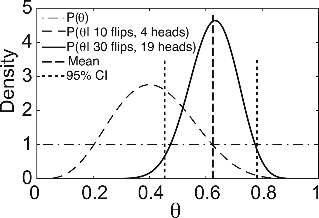
Third, given new experimental data, Bayes’ theorem updates the likelihood of the possible parameter values using the prior distribution and the likelihood function. The resulting distribution, called the posterior probability, provides the likelihood of each possible parameter value, given both our prior knowledge and experimental data. In the coin experiment, suppose 4 out of 10 flips were heads. Combining the prior with the outcome of this experiment produces the posterior distribution shown in Figure 1. Note how the belief in the possible values of θ has shifted away from the uniform prior and towards a distribution with a mean near 0.40 as suggested by the experimental data. That is, there is a high likelihood that θ is near 0.40, but little chance that θ ≥ 0.85. The posterior can be updated when more data become available. If the coin is flipped 20 more times with 15 heads, the posterior is now centered near 0.63 (i.e., 4 + 15 = 19 heads out of 10 + 20 = 30 flips). As more data are collected, the influence of the prior decreases and the posterior becomes narrower, indicating greater confidence in certain parameter values.

Figure 1.

Coin-flip illustration of Bayesian statistical concepts. In this example, the prior probability distribution P(θ) is the uniform distribution on [0,1], and P(θ | 10 flips, 4 heads) is the posterior distribution resulting from the experiment that yielded 4 heads out of 10 coin flips. The posterior P(θ | 30 flips, 19 heads) was computed using the experimental outcomes of a total of 30 flips, and is shown as a solid curve with the mean as a dashed vertical line and the 95% CI indicated with dotted vertical lines.

Once the posterior probability distribution is calculated, it is possible to determine any statistic of interest for the parameters, e.g., the mean, the standard deviation, the mode, and so on. For example, the mean estimate of θ after 30 flips, 0.625, shown in Figure 1, is the mean of the posterior probability distribution. Note that, because of the influence of the prior, this value is still slightly lower than the data mean of 0.63. (See (Kruschke, 2011) for a friendly introduction to Bayesian statistics and a more detailed description of this coin problem.)

Bayesian statistics allows us to quantify how confident we are in our estimation of parameter values. The credible interval (CI) is a measurement of the uncertainty associated with a parameter estimate. The CI is the Bayesian equivalent of a confidence interval. Unlike a standard confidence interval, however, the interpretation of a CI is straightforward: the probability that a parameter lies within a 95% CI is 0.95. The margin of error is defined as half the width of a CI. There are a few different ways to define a CI. Here we follow the most common practice and simply take the middle 95% of the posterior probability distribution. The 95% CI for the 30 trial coin-flipping example is provided in Figure 1.

It is commonly difficult or impossible to produce an analytical solution to determine the posterior probability. It is, however, often possible to determine the posterior to within a scaling constant, that is, we only have access to an un-normalized form of the posterior. From this un-normalized function it is possible to determine the relative likelihood of each parameter value, but, without the normalizing factor, it is not possible to directly draw samples or determine statistics from it. Thus, stochastic methods have been developed to numerically approximate the posterior. Arguably the most important class of such methods is Markov chain Monte Carlo (Gamerman, 1997; Hastings, 1970) in general and the Metropolis Hastings (MH) algorithm (Chib and Greenberg, 1995) in particular. The key idea behind the MH algorithm is to draw samples from a carefully chosen, easy-to-sample distribution, called the proposal distribution, and then to use the relative likelihood provided by the un-normalized posterior to accept or reject these samples as proposed samples from the posterior. The proposal distribution must satisfy certain properties. For example, the proposal distribution must be non-zero everywhere the posterior is non-zero. See (Andrieu et al., 2003) for an accessible overview of rejection sampling, the MH algorithm, and MCMC in general. The set of accepted samples can then be used to approximate the posterior distribution and thereby estimate statistics on the parameter. Because these distributions are built up from a set of discrete samples, they typically look more like histograms than the smooth distributions of Figure 1. Software such as OpenBUGS (mathstat.helsinki.fi/openbugs/) is readily available for running MCMC methods.

Because practical implementation requires fast computers, the Bayesian estimation of frequency is a relatively young field. Jaynes (1987) and Bretthorst (1988) clarified the relationship between Bayesian inference, spectral analysis, and parameter estimation, and derived the earliest methods of Bayesian spectral analysis. In particular, Bretthorst (1988) used a Bayesian framework to show that the peak frequency of the Schuster periodogram is the optimal estimator under the assumption of a single sinusoid plus white noise, as well as deriving a generalized framework for Bayesian spectral analysis. Dou and Hodgson (1995) developed an MCMC algorithm for estimating period, phase, and amplitude of multiple sinusoids. Andrieu and Doucet (1999) developed an approach based on the MH algorithm that is more efficient than earlier methods and remains robust when the signal-to-noise ratio is low, and that is extended to a dynamic sinusoidal model in (Nielsen, 2009; Nielsen et al., 2011).

To apply a Bayesian analysis to the study of the period of biological oscillators, we follow the procedure described in (Andrieu and Doucet, 1999; Nielsen, 2009; Nielsen et al., 2011), to which we give the acronym BPENS (Bayesian parameter estimation for noisy sinusoids). Following the steps outlined above in the coin-flipping example, we must first specify a data model and then derive its likelihood function. A natural data model for a biological oscillator is a noisy sinusoid

$$x=A\text{ cos}(\mathrm{\omega }t+\mathrm{\phi })+{\epsilon }_t.$$

Here A is the amplitude, φ is the phase angle, ω is the frequency, t is time, and ε_t represents noise at time t. We assume ε_t at each time point to be independent and identically distributed Gaussian noise with mean 0 and variance σε², that is, ε_t = N(0, σε²). We can express this model in the equivalent form

$$x=B_1\text{ cos}(\omega t)+B_2\text{ sin}(\omega t)+{\epsilon }_t.$$

Because a parameter is removed from inside the cosine function, this form is mathematically more convenient. A likelihood function is then derived from this equation. The likelihood function gives the probability that this data model with particular values for parameters ω, B₁, B₂, and σε could produce the observed time series {x(t_i): i=1,…,N}. Chapter 4 of (Nielsen, 2009) provides a derivation of the likelihood function associated with the noisy sinusoid model, which is too technical to include here; also see (Andrieu and Doucet, 1999).

The second step is to select prior distributions for the parameters. We use the mathematically convenient priors given in (Andrieu and Doucet, 1999) and (Nielsen, 2009). For example, the prior distribution of ω is assumed to be a uniform distribution from 0 to π radians/time unit, meaning that all possible frequency values are judged equally likely a priori. See Appendix C for details on the choice of prior distributions, and (Bretthorst, 1988) for a general discussion of how to select prior distributions.

The third step is to determine the posterior distribution of the frequency parameter ω, which gives the probability of particular values for ω given the observed time series. Given experimental data, i.e., a time series, the prior distributions, and the likelihood function, Bayes’ theorem yields an expression for the posterior distribution. The posterior is proportional to the product of the prior distributions and the likelihood function. Because the posterior contains an unknown scaling constant, the MH algorithm is used to approximate the normalized posterior (with the scaling constant divided out). Statistics of interest can then be derived from this approximated posterior. Specifically, the mean of this distribution provides a point estimate of frequency and the CI provides a measure of uncertainty. The parameters B₁, B₂, and σε are considered nuisance parameters, and are removed by integrating the Bayes’ Theorem expression with respect to each of these parameters. A potential downside of the BPENS method is that, compared to the other methods described below, it is relatively time consuming.

1.2 Summary of other period estimation methods

We next briefly survey some methods in common use for estimating period of biological oscillations, particularly for circadian rhythms.

Direct sine-fitting calculates the amplitude, period, and phase angle for the sine curve that best fits the data (sometimes including an exponential decay term for the amplitude). This method is most appropriate for sinusoidal waveforms, such as circadian clock gene expression rhythms measured using PER2::LUC reporter bioluminescence. Similar to BPENS, sine-fitting methods offer a measure of uncertainty in the form of a confidence interval or margin of error (half the width of the confidence interval) for the period estimate, but these values are, unfortunately, rarely reported. In place of confidence intervals, researchers often rely on goodness-of-fit. However, goodness-of-fit indicates how sinusoidal the time series is, rather than giving a direct indication of how reliable the period estimate is. The period estimate from a model fit with a goodness-of-fit value of R²=0.95 could be less reliable than one for a different time series with R²=0.9 if, for example, the lower R² value is due to the latter time series having a significant trend or non-sinusoidal waveform despite exhibiting strong periodicity.

All of the remaining methods provide point estimates for the period but no measure of uncertainty.

The discrete Fourier transform (DFT) decomposes a signal into a sum of sinusoids, with the Fourier coefficients giving the amplitude associated with each frequency. Numerical methods, including the fast Fourier transform (FFT) and windowed variants, offer period point estimates for a variety of data types. Because the frequencies for the DFT are uniformly spaced by 1/T cycles/hour, where T is the length of the time series in hours, the point estimate will have poor resolution unless the time course is reasonably long. For example, the DFT of a time series 4 days in length will report frequencies in the circadian range corresponding to 19.2h, 24.0h, and 32.0h periods. For a time series 32 days in length, the resolution improves but is still limited, having values 22.59h, 23.27h, 24.0h, 24.77h, and 25.6h in the 22–26h range. Although the point estimate resolution is poor, the DFT can be used very effectively to detect whether a significant rhythm is present and to measure the strength of rhythmicity (Ko et al., 2010; Leise et al., 2012).

Maximum spectral entropy analysis (MESA) fits an autoregressive function to the data and uses the coefficients to calculate the power spectrum with substantially better resolution than the Fourier transform can offer. MESA can work quite well on even short noisy time series, but does not provide a test for significance of the rhythm at a peak frequency (Dowse, 2009).

The coefficients of the autocorrelation sequence (ACS) give the correlation between a time series and shifted versions of itself. A peak in the ACS occurs when the time series is shifted by its period, thereby yielding a simple technique for detecting significant periodicity (Dowse, 2009). If low frequency trend is first removed, this method can provide good point estimates of circadian period, even for non-sinusoidal locomotor activity data.

The chi-square periodogram, a method often used to assess circadian rhythmicity of non-sinusoidal locomotor activity records, essentially rasterizes or folds data, averaging together data points separated by a given time interval to yield an educed waveform for each period value, and then choosing the period resulting in the maximum variance of waveform values. Unfortunately this method suffers from contamination by harmonics and subharmonics and can be misleading in some cases, for example, mistakenly categorizing noisy rhythmic data as arrhythmic (Dowse, 2009).

Another approach is to identify discrete phase markers such as peaks in bioluminescence data or onsets in activity records. The average time between such phase markers can be used as a point estimate of the period. For PER2::LUC bioluminescence, the mean peak-to-peak times can produce good estimates if the time series is first smoothed, which is often done using a running average.

Period point estimates produced by most of these methods can be improved by first filtering the data. Many methods are available to remove a linear trend or smooth the data to reduce high frequency noise. A particularly effective method is to apply discrete wavelet transforms to remove high and low frequencies to extract the circadian component of a time series, thereby smoothing the signal and removing nonlinear trends without distorting the circadian frequency content (which is a danger of removing high order polynomial trends).

Because calculation of peak-to-peak times to estimate circadian period can be improved by first applying a stationary discrete wavelet transform (Leise and Harrington, 2011), we report this method in addition to the peak-to-peak estimate obtained from smoothing with a running average.

2. RESULTS

2.1 Comparison of the accuracy of point estimates

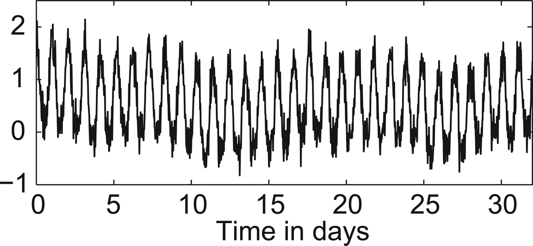
Before we examine the question of uncertainty in an individual period estimate, we compare the accuracy of point estimates generated by our BPENS method and the six commonly used methods described above. Each method is applied to 100 simulated noisy oscillatory time series of different lengths with a known period of 24.9h that mimic the experimental data (see Appendix A). See Figure 2 for an example. For each method, the absolute difference between the true period and the estimated period averaged over the 100 simulations is given in Table 1. Note that this procedure tests how close the estimated period is to the true period, which is a distinct issue from the uncertainty of an individual period estimate for a time series of unknown period (as occurs in the experimental context as discussed below). For all methods, accuracy tended to increase with the number of cycles in the time series. Of the seven methods tested, the BPENS method yielded the most accurate period estimates and consistently generated fairly accurate values even for the short 4-cycle time series. We also tested the sensitivity of the different methods to noise by comparing the errors for different levels of noise in the simulated time series, shown in Table S1. For most methods, error tends to increase with noise level.

Figure 2.

Example of simulated noisy oscillatory time series used to test the 7 period estimation methods.

Table 1.

Comparison of methods to determine period in simulated noisy oscillatory time series of various lengths and a sampling rate of 2 samples/h, where the true period is 24.9h. Values in the table are the absolute error averaged over the 100 point estimates for each of the 7 methods.

Length of time series	DFT	MESA	ACS	Peak-to- peak (running average)	Sine-fitting	Peak-to-peak (wavelet)	BPENS
4 cycles	36 min	15 min	23 min	31 min	13 min	7.6 min	5.4 min
8 cycles	28 min	6.2 min	8.4 min	7.1 min	1.7 min	3.3 min	1.7 min
16 cycles	28 min	1.3 min	8.1 min	2.3 min	1.6 min	0.93 min	0.61 min
32 cycles	16 min	0.65 min	6.0 min	2.1 min	0.42 min	0.53 min	0.24 min

We can further validate the accuracy of the BPENS method by comparing its results for real experimental data with those of the wavelet-filtered peak-to-peak method. The peak-to-peak method was selected for comparison because it is distinct from the sine-fitting methods and performed well in the simulation test. For the fibroblast time series (Leise et al., 2012), the peak-to-peak and BPENS methods produced strongly correlated period estimates (r=0.96, p<0.001), indicating that BPENS estimates are consistent with those of an established method. Although the noisy sinusoid model underlying BPENS is appropriate for our fibroblast data, methods not based on sinusoidal models may be more accurate for time series with different waveforms.

2.2 Comparison of uncertainty measures

Recall that both the sine-fitting and the BPENS method provide measures of uncertainty for individual time series. We compare the margin of error for the two methods applied to the 24.9h simulated data, with results in Table 2. Because they have different theoretical interpretations, direct comparison of the margins of error produced by these two methods would not be appropriate. Therefore, we instead take a frequentist approach and compare the number of times that the true period lies within the estimated margin of error. The two methods yield similar results, with the exception that BPENS provides a more conservative assessment of the uncertainty when given only 4 cycles of data (as shown in Table 2) but in all cases a more accurate point estimate of the period (as shown in Table 1). Noise level in the simulated signals had little effect on the BPENS estimated margin of error, as shown in Table S2.

Table 2.

Comparison of margin of error computed using the two different methods, sine-fitting (using Matlab’s Curve Fitting Toolbox) and BPENS, for the 100 simulated noisy oscillatory time series. The margin of error equals half the width of the 95% CI. The percent of samples in which the estimated period value was within the 95% CI is given in parentheses.

Length of time series	Sine-fitting	BPENS
4 cycles	17 min (71%)	48 min (100%)
8 cycles	7.1 min (99%)	13 min (100%)
16 cycles	3.2 min (98%)	3.5 min (100%)
32 cycles	1.3 min (99%)	1.0 min (100%)

2. 3 Uncertainty in fibroblast time series period estimates and its relation to the number of observed cycles

The previous analysis demonstrates that the accuracy of the BPENS method is superior for determining period point estimates (for time series similar in nature to the test data). We now describe how the BPENS method can be used to determine the uncertainty in these period estimates in experimental data. We expect uncertainty to depend on properties of the experimental time series, such as the length of the series and signal-to-noise ratio. Under the assumption of a sinusoid plus white noise with known variance, Bretthorst (1988) derived an expression for the frequency estimate that shows that uncertainty decreases as the signal-to-noise ratio increases and as N, the number of data points, increases. By increasing the number of cycles or the sampling rate, we increase N and so reduce the uncertainty in the period estimate. Similarly, we can more reliably estimate the period of a time series with a larger signal-to-noise ratio. See Appendix F for details. For the experimental data we consider, the assumptions necessary for this derivation do not hold, so we numerically calculate the uncertainty.

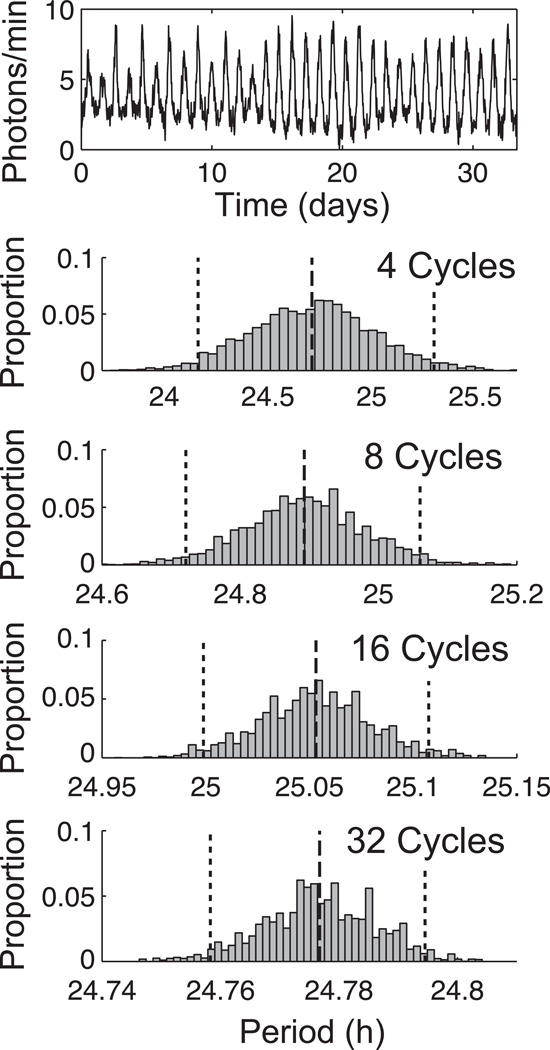
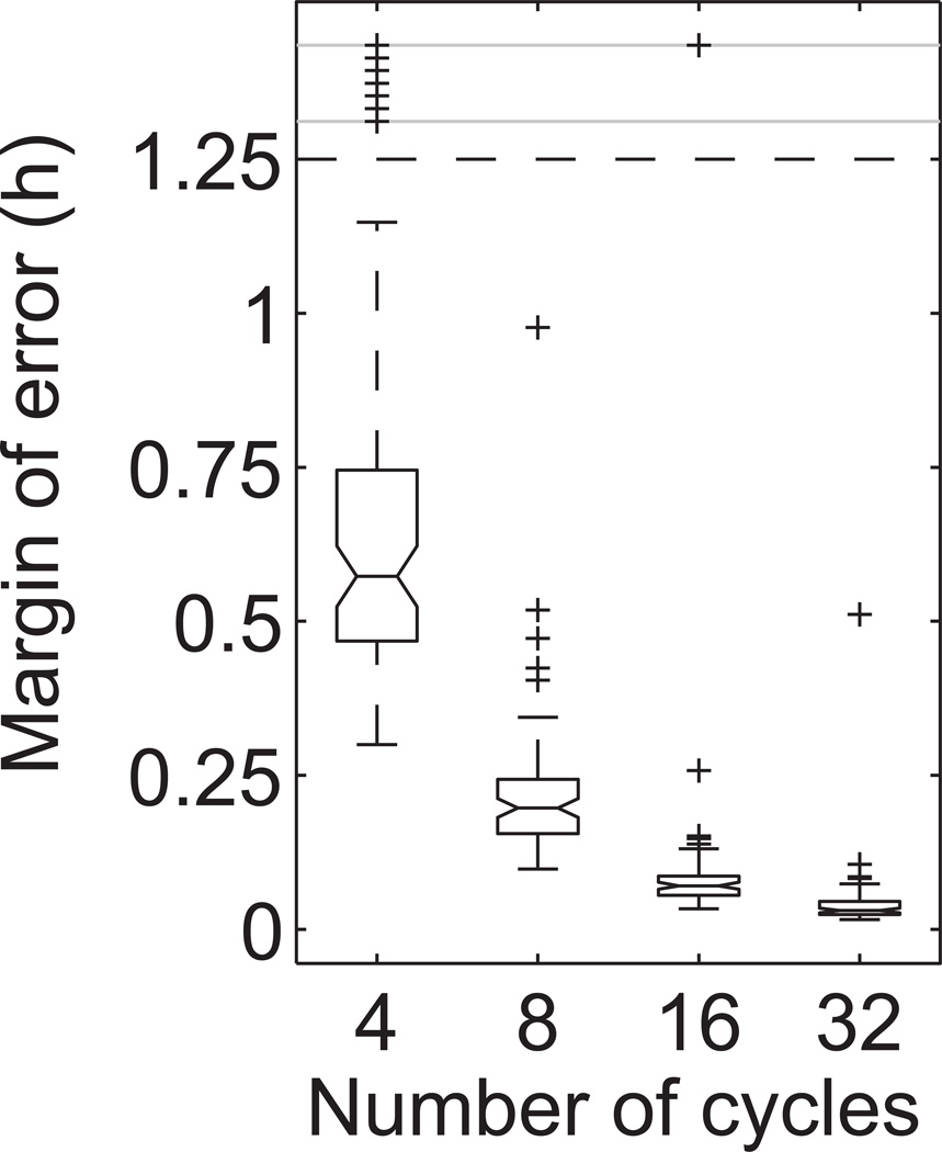
We applied the BPENS method to a set of PER2::LUC recordings of 78 dispersed fibroblasts from mice reported previously (Leise et al., 2012). The objective is to measure uncertainty in the period estimates and use these results to determine the length of recording necessary for accurate and reproducible period estimation for this type of noisy biological oscillator. Figure 3 shows the posterior distributions for the period computed by the BPENS method for a representative fibroblast using 4, 8, 16, and 32 cycles. Note that the reliability of the period estimate increases with the number of cycles. In this example, the margin of error is 0.57h, 0.17h, 0.054h, and 0.018h for 4, 8, 16, and 32 cycles, respectively. Figure 4 provides the distribution of margins of error for the four different lengths of times series. In general, the margin of error decreases toward zero as the time series lengthens.

Figure 3.

Application of the BPENS period estimation method to Fibroblast #57, whose time series is shown at the top, using 4, 8, 16, or 32 cycles. Each histogram displays the computed posterior distribution for the period, with 95% CIs indicated by dotted lines and the mean value by a dashed line. The width of the CIs reflects the uncertainty of the period estimate. Note that as the number of cycles increases, the range of the horizontal axis greatly decreases.

Figure 4.

Box plot of the margins of error for the fibroblast time series versus the number of cycles in the time series. Median margins of error are 0.57h, 0.20h, 0.071h, and 0.031h for 4, 8, 16, and 32 cycles, respectively. Plus signs indicate outliers.

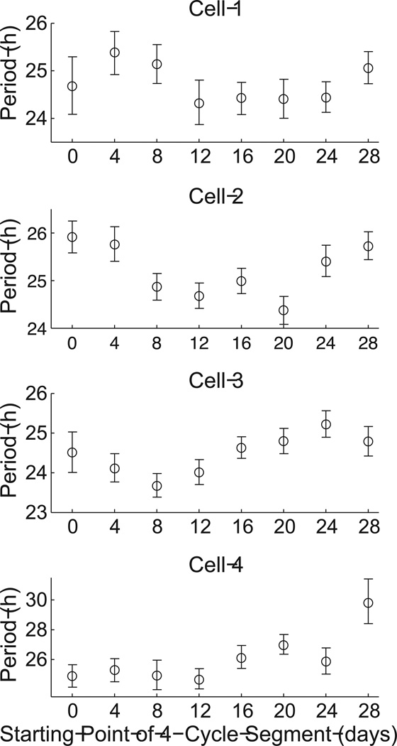
Note that, for the fibroblast shown in Figure 3, using only the first 4 cycles yields a somewhat different mean period estimate than when using 32 cycles. This outcome is a consequence of the stochastic variability in period across the 32 cycles. That is, the length of each cycle varies over time. Because a short time series captures only a small random sample of the cycle lengths, it will be less representative of the full distribution of cycle lengths that can occur. Figure 5 illustrates how period estimates can vary over time for 4 fibroblast examples.

Figure 5.

Estimated period for 4-cycle segments of four fibroblast time series starting at different time points, revealing variability in estimated period over time. Cells 1–4 are Fibroblasts #57, #25, #44, and #65, respectively (Leise et al., 2012). Error bars show 95% CIs and the mean is marked with a circle.

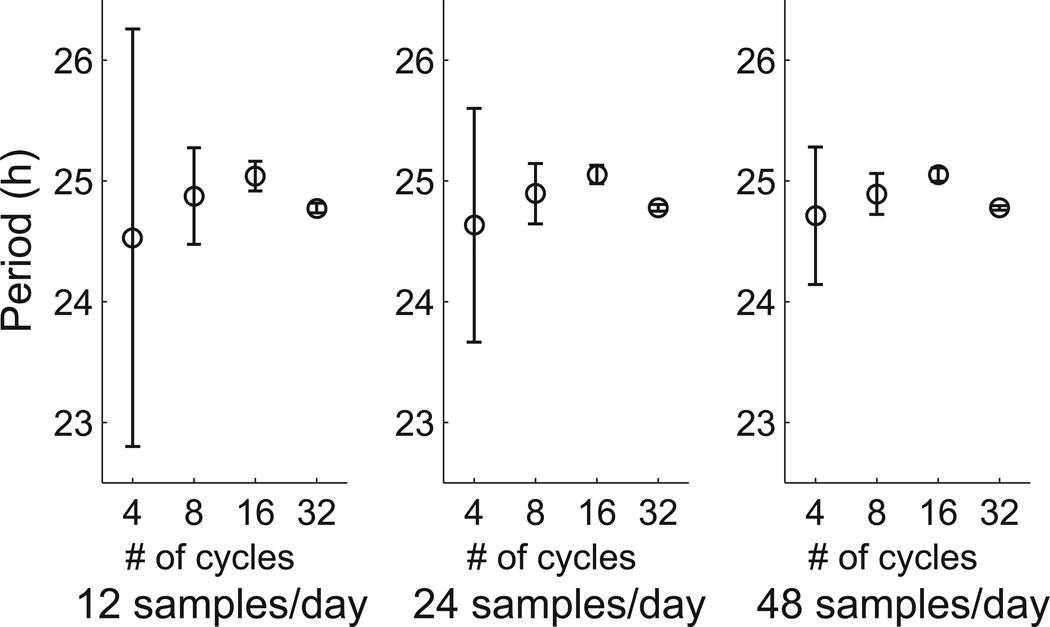
Because experiments also vary in how often measurements are recorded, we examined different sampling rates. Figure 6 illustrates how sampling rate affects uncertainty in the period estimate. For all sampling rates, the margin of error decreases with the number of cycles in the time series. In addition, the margin of error also decreases as sampling rate increases. The number of cycles had a much greater effect than sampling rate, consistent with the theoretical analysis in Appendix F; sampling rate only had a strong effect when the number of cycles was low. Regardless of the sampling rate, 16 cycles appears sufficient to yield quite reliable estimates under the BPENS method.

Figure 6.

Effect of the number of cycles and sampling rate on the uncertainty in the BPENS period estimate for Fibroblast #57. Error bars are 95% CIs with the mean marked. The margin of error decreases as the number of cycles and the sampling rate increase.

2.4 Reliable determination of the population’s mean period

We assume that each oscillator has an intrinsic period that may differ from those of others in the population and so we must consider not only stochastic variability over time within each cell, but also variability across the population of cells. How many cells and how many cycles do we need to estimate the mean period of the population to a given level of accuracy? That is, how will the uncertainty in the mean period estimate for a population of cells vary with the number of cells and the number of cycles?

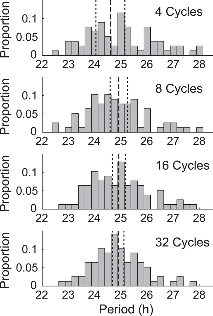
BPENS was used to calculate a point estimate of the period for each of the 78 fibroblasts for 4, 8, 16, and 32 cycles. Histograms of these point estimates are shown in Figure 7. The mean of these point estimates was taken as an estimate of the population’s mean period. A 95% confidence interval can then be constructed for the population’s mean period. The estimate of the population’s mean period and associated confidence interval are also shown in Figure 7. Three trends emerge from this analysis. First, the estimate of the mean period of the population remains consistent when using 8 or more cycles per cell. Second, as more cycles are used, fewer outliers appear. Third, uncertainty in the mean period decreases as the number of cycles increases. Varying sampling rate had little effect on either this or the following analysis and so is not reported.

Figure 7.

Histograms with 15 min bins showing the estimated mean fibroblast periods using the BPENS method. Dashed lines indicate the mean value of the mean periods for 78 fibroblast time series; the dotted lines give the 95% CIs for the mean of the mean periods. 7 outliers in the 4 cycles histogram and 3 outliers in the 8 cycles histogram are not shown.

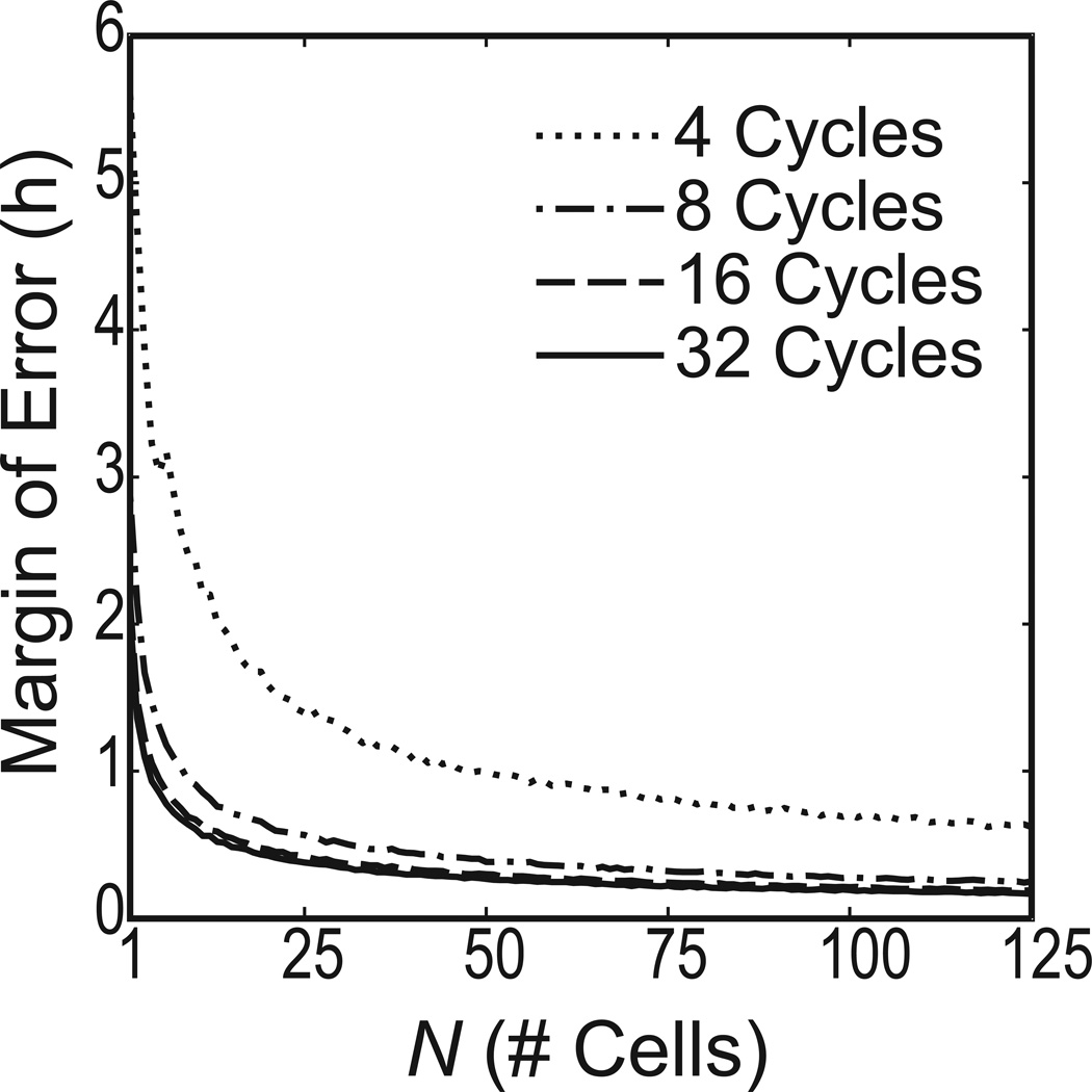
The analysis above varied the number of cycles for a fixed number of cells. Given a fixed number of cycles, we can extend this procedure to estimate how many cells are needed to reach a desired CI width. We sampled with replacement from the 78 cell periods estimated by BPENS for a fixed number of cycles. The number of cells sampled was varied. This bootstrapping procedure was repeated 5000 times. Figure 8 shows the margin of error resulting from the 5000 bootstrap samples, for each sample size. For example, with only 4 cycles, we need approximately 194 cells to reduce the margin of error to 30 min, but with 32 cycles the required number of cells drops to 14. This analysis provides a guideline for determining the number of cells and cycles that should be recorded in similar experiments to yield reproducible period measurements. Table 3 shows the number of cells required to achieve a margin of error of 0.5h, 0.25h, or 0.125h for 4, 8, 16, or 32 cycles.

Figure 8.

The number of cells (N) required to achieve the desired margin of error for the mean period of the population, given the number of cycles recorded (using 48 samples/day). The margin of error decreases as the reciprocal of the square root of the number of cells.

Table 3.

Number of cells required to achieve a margin of error of 0.5h, 0.25h, or 0.125h, given experimental time series of different lengths.

Length of time series	0.5h	0.25h	0.125h
4 cycles	194	770	3073
8 cycles	31	124	494
16 cycles	18	71	283
32 cycles	14	58	231

2.5 Decomposition of within-cell and between-cells variability to assess heterogeneity in the population

Once a good estimate of the population’s mean period is obtained, the next natural question concerns the variability in the cell periods. Consider the dataset of BPENS period estimates consisting of 8 consecutive, non-overlapping 4-day segments from each of the 78 cells. We can ask whether the intrinsic periods of all 78 oscillators are similar, with noise causing the apparent differences, or whether the population is heterogeneous with some distribution of periods. To address this question, we turned to a Bayesian hierarchical model to estimate simultaneously the variability across cells and the variability of period over time within each individual cell.

The model assumes that the intrinsic periods of the cells are normally distributed with population mean μ and standard deviation ρ. We further assume that each cell’s time series exhibits some level of variability in cycle length. That is, each cell’s period is normally distributed about its intrinsic period with some standard deviation σ. A numerical parameter estimation procedure involving the MH algorithm similar to that described above was used to determine values for the three parameters μ, ρ, and σ (see Appendix E). Figure 9 provides the posterior probabilities for each of these parameters. In agreement with the results above, the best estimate of the population’s mean period, μ, is 24.94h, with CI [24.72,25.17]. The standard deviation of periods across the population, ρ, is 0.89h, with CI [0.72,1.09]. The within-cell variability, σ, is 1.43h, with CI [1.34,1.51].

Figure 9.

Hierarchical modeling of the 78 fibroblasts. The dashed lines mark the mean values and the dotted lines indicate the 95% CIs for the parameters μ (mean period of the population), ρ (standard deviation of periods across the population), and σ (standard deviation in cycle length for each cell).

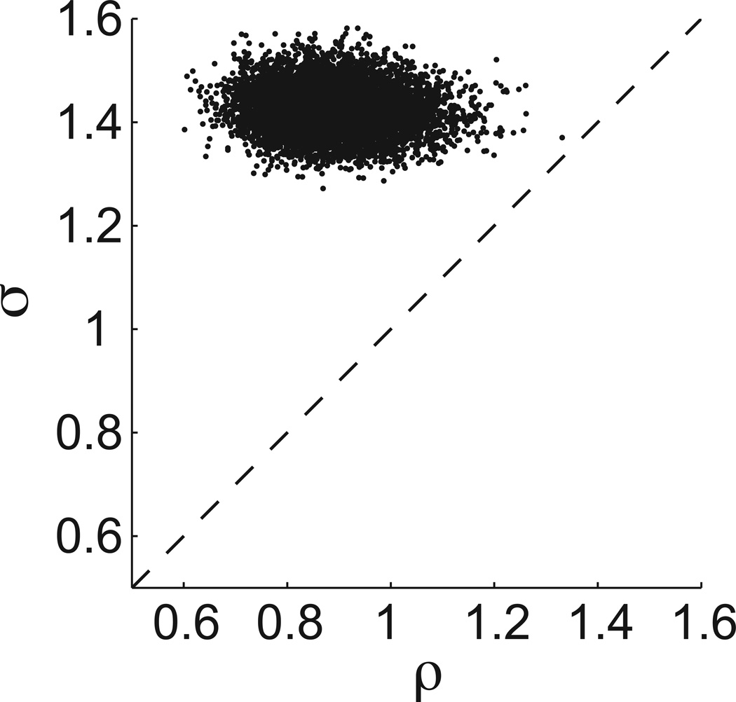
This result provides an estimate of the heterogeneity in the population of cells. As in a standard ANOVA, the magnitude of the between-cell variability, ρ, is best viewed in relation to the within-cell variability, σ. Because the posterior distributions of ρ and σ are not independent, we need a measure of how these parameters co-vary. Figure 10 provides a set of 8,000 samples drawn from the joint distribution of ρ and σ, numerically generated by the MH algorithm. For this set of samples, ρ is always less than σ, implying that the between-cell variability is less than the within-cell variability.

Figure 10.

Scatter plot of 8,000 samples drawn from the joint distribution of ρ and σ. The between-cells variability ρ is less than the within-cell variability σ for the set of 78 fibroblasts.

We have assumed that within-cell variability involves fluctuations about some intrinsic period for each individual oscillator, but a potential issue is that the period of the cell population could change gradually over the duration of an experiment due to declining health of the cells or changes in the medium. This appears to be only a minor concern for our fibroblasts, as the mean period across the population shows only a very gradual increase of 0.02 h/day, or 0.1% per day, as reported in (Leise et al., 2012).

3. DISCUSSION AND CONCLUSIONS

As a consequence of both intrinsic noise from the molecular dynamics of the intracellular clock and extrinsic noise from other processes inside and outside the cell, cellular oscillators exhibit fluctuations in frequency (Elowitz et al., 2002; Gonze et al., 2002). In particular, short recordings with few cycles may yield misleading results: overestimation of population heterogeneity, large potential error in the estimated period of each cell, and difficulty in assessing which cells are significantly rhythmic (Leise et al., 2012). On the other hand, practical constraints for experiments limit how many cycles can be recorded. For circadian oscillations in fibroblasts, our analysis suggests that 16 cycles is sufficient to generate reliable point estimates for individual cell periods using the BPENS method. The stochastic cycle-to-cycle variability illustrated in Figure 4 implies that short time series with only 4 or even 8 cycles may yield erroneous estimates of the cell’s intrinsic period.

In addition to cycle-to-cycle variability in individual biological oscillators, a population of genetically similar oscillators can exhibit a range of periods due to a combination of within-cell and between-cell variability. It is important to distinguish the effects of variability due to stochastic gene expression from heterogeneity in the population due, for example, to differences in cell size or epigenetic changes. Our hierarchical modeling reveals that, while there is some heterogeneity of intrinsic period in the population, the fibroblasts display much greater within-cell variability than between-cell variability in period. This finding agrees with the ANOVA results in (Leise et al., 2012), which used period estimates generated by the wavelet-based peak-to-peak method.

For the fibroblast time series considered here, which exhibited stable circadian oscillations, a simple single-frequency model was sufficient. However, in some situations, such as a forced desychrony protocol (de la Iglesia et al., 2004), two or more periods may be present in the time series, in which case the full multiple-sinusoid reversible jump MCMC algorithm developed by Andrieu and Doucet (1999) would be appropriate. This algorithm is designed to detect how many significant rhythms are present and then estimate their frequencies, and it outperforms classical model selection techniques like the Akaike Information Criterion in assessing the number of significant components. In the case of an oscillator for which the period is expected to change significantly over time, a dynamic sinusoidal model as treated by Nielsen et al. (2011) or probabilistic inference of instantaneous frequency as in (Turner and Sahani, 2011) may be more appropriate.

We conclude that BPENS is a general, powerful method for determining period of oscillatory time series, including short noisy time series, which generates both accurate point estimates and a measure of uncertainty. Commonly used methods, including the FFT, MESA, autocorrelation, and mean peak-to-peak time, provide less accurate period estimates than BPENS and no information about uncertainty of the estimate. Thus, BPENS permits not only the best available estimate of oscillatory period, but also an opportunity to evaluate the reliability of point estimates based on noisy experimental data. By taking uncertainty into account, one can calculate the number of cycles required to attain a desired precision of period estimation and thereby be confident that experimental findings are reliable and reproducible.

Highlights.

• The method provides more accurate period estimates than other common methods.

• It also quantifies the reliability of period estimates of noisy oscillators.

• Cellular oscillators exhibit significant stochastic variability in period.

• We assess the length of time series required for reliable period estimation.

• Hierarchical modeling distinguishes within-cell from between-cell variability in period.

Appendix A

Simulated data generation

The simulated time series were generated by sampling a modified waveform (at 0.5h intervals) consisting of the constant ½ plus a cosine function with period 24.9h and unit amplitude, with portions falling below zero set equal to zero, and then adding both Gaussian and Brownian noise, each with standard deviation 0.2 (to mimic experimental time series; see Figure 2 for an example). Because they have more low frequency noise and an altered waveform, these simulated time series have properties differing from a simple sinusoid with additive noise.

Appendix B

Fibroblast data

The complete set of experimental data can be found in the Supporting Information of (Leise et al., 2012). We used 34 days from each recording (starting at the 4^th peak), in order to obtain 32 cycles on average for each cell (the typical cycle length is approximately 25h). Each time series was detrended using a stationary discrete wavelet transform as described in (Leise and Harrington, 2011). Because they were too short for this analysis, we discarded cells #42 and #61 from the original set of 80 fibroblast time series.

Appendix C

BPENS parameters

Determining the posterior distribution for the frequency parameter ω follows algorithm 4.2 of (Nielsen, 2009) with the following parameter values: T = 10,000, λ = 0.2, g= 6, a = 5, b= 60, and σ² = (.5/N)², where N is the number of data samples. The initialization value for the MH algorithm was 25 hours. The algorithm was robust to different starting values and parameter values for the prior distribution. Burn-in time was 20% of total accepted samples. T is the number of total samples. The form of the prior follows equation (4.26) in (Nielsen, 2009), in which the assumed factorization is the least subjective prior distribution in the absence of prior knowledge, as shown in (Andrieu and Doucet, 1999). The distribution of ω is assumed to be a uniform distribution from 0 to π radians/time unit, while the distribution of σε² is the inverse-Gamma function Inv-G(σε²; a,b), which is the conjugate prior for a Gaussian distribution with known mean and unknown variance. The prior for the amplitude parameter B is the normal distribution with mean zero and variance depending on σε², ω, and the expected signal-to-noise ratio g. The proposal distribution is a mixture of the normalized Fourier periodogram and a Gaussian with variance σ². The mixing parameter is λ.

Appendix D

Description of other period estimation methods

For the sine-fitting method, simulated time series with linear trend removed were fit to a single sine function using the MATLAB Curve Fitting Toolbox (MathWorks, Inc., Natick, MA, 2011), which uses nonlinear least squares with a trust-region algorithm. The simulated time series also had linear trend removed before applying MESA and Fourier periodogram methods, while before applying autocorrelation the simulated time series were wavelet-detrended as described in (Leise and Harrington, 2011). The first peak-to-peak method used a 12h running average to smooth before selecting peak times, and the second peak-to-peak method applied the wavelet-based procedure described in (Leise and Harrington, 2011).

Appendix E

Hierarchical model

The hierarchical modeling follows the procedure in Section 8.3 of (Hoff, 2009). We assumed a fixed variance σ² for each group. Priors were 1/σ² ~ γ(ν₀/2, ν₀ σ₀²/2), 1/ρ² ~ γ (η₀/2, η₀ρ₀²/2), μ ~ N(μ₀, γ₀²); within-group model: φ _j = { θ _j, σ²}, p(y | φ _j) = N(θ _j, σ²); between-group model: ψ = {μ, ρ²}, p(θ_j | ψ) = N(μ,ρ²). Parameter values were ν₀=1, σ₀²=2, η₀=1, ρ₀²=3, μ₀=25, γ₀²=0.25. 10,000 samples were used in the MH algorithm and burn-in time was 20% of total accepted samples. Because each cell has only 8 observations and to keep the number of parameters reasonable, we assumed all cells had the same value of σ.

All computations were done using MATLAB R2011b (MathWorks, Inc., Natick, MA, 2011).

Appendix F

Theoretical uncertainty of Bayesian frequency estimates

Bretthorst (1988) used a Bayesian framework to show that the peak frequency of the Schuster periodogram is the optimal estimator under the assumption of a single sinusoid B₁cos(ωt) plus white Gaussian noise with known variance σ². The Schuster periodogram C(ω) is defined by

$$C(\omega )=\frac{1}{N}{\left|{\displaystyle \sum _{j=1}^N}{x}_j{e}^{i\omega t_j}\right|}^2.$$

The value ω’ at which C(ω) attains its maximum is the best estimate. Using this approach and under these assumptions, Bretthorst, following (Jaynes, 1987), derived a closed-form expression for the frequency estimate and its standard deviation:

$$f_{\mathit{\text{est}}}=f\prime \pm \frac{1.1\sigma }{B_{1}T\sqrt{N}}(\text{in cycles}/\text{time unit}),$$

where f=ω/(2πΔt), Δt is the sampling time step, T is the total duration of the time series, and N is the number of sampled time points. This expression shows that the uncertainty in the frequency estimate is inversely proportional to the signal-to-noise ratio (B₁/σ), so increasing the signal-to-noise ratio should reduce the uncertainty in the frequency estimate. We also see that doubling the number of cycles recorded (thereby doubling both T and N) will have a greater effect in reducing the uncertainty than doubling the sampling rate (which only doubles N and not T). Because we don’t know σ for the fibroblast time series, we cannot directly use this expression, but our experimental results are consistent with this theoretical analysis.

REFERENCES

- Andrieu C, Doucet A. Joint Bayesian model selection and estimation of noisy sinusoids via reversible jump MCMC. IEEE Transactions on Signal Processing. 1999;47:2667–2676. [Google Scholar]
- Andrieu C, N DF, Doucet A, Jordan MI. An introduction to MCMC for machine learning. Machine Learning. 2003;50:5–43. [Google Scholar]
- Bell-Pedersen D, Cassone V, Earnest D, Golden S, Hardin P, Thomas T, Zoran M. Circadian rhythms from multiple oscillators: Lesson from diverse organisms. Nat Rev Genet. 2005;6:544–556. doi: 10.1038/nrg1633. [DOI] [PMC free article] [PubMed] [Google Scholar]
- Bretthorst GL. Bayesian Spectrum Analysis and Parameter Estimation (Lecture Notes in Statistics 48) Berlin: Springer; 1988. [Google Scholar]
- Chib S, Greenberg E. Understanding the Metropolis--Hastings algorithm. The American Statistician. 1995;49:327–335. [Google Scholar]
- de la Iglesia HO, Cambras T, Schwartz WJ, Díez-Noguera A. Forced desychronization of dual circadian oscillators within the rat suprachiasmatic nucleus. Curr Biol. 2004;14:796–800. doi: 10.1016/j.cub.2004.04.034. [DOI] [PubMed] [Google Scholar]
- Dou L, Hodgson RJW. Bayesian inference and Gibbs sampling in spectral analysis and parameter estimation: I. Inverse Problems. 1995;11:1069–1085. [Google Scholar]
- Dowse H. Analyses for physiological and behavioral rhythmicity. In: Johnson ML, Brand L, editors. Methods in Enzymology. Vol. 454. Burlington: Academic Press; 2009. pp. 141–174. [DOI] [PubMed] [Google Scholar]
- Dunlap JC, Loros JJ, DeCoursey PJ, editors. Chronobiology: Biological Timekeeping. Sunderland, MA: Sinauer Associates, Inc; 2004. [Google Scholar]
- Elowitz MB, Levine AJ, Siggia ED, Swain PS. Stochastic gene expression in a single cell. Science. 2002;297:1183–1186. doi: 10.1126/science.1070919. [DOI] [PubMed] [Google Scholar]
- Gamerman D. Markov Chain Monte Carlo (Texts in Statistical Science) New York: Chapman & Hall; 1997. [Google Scholar]
- Gonze D, Halloy J, Goldbeter A. Robustness of circadian rhythms with respect to molecular noise. Proc Natl Acad Sci USA. 2002;99:673–678. doi: 10.1073/pnas.022628299. [DOI] [PMC free article] [PubMed] [Google Scholar]
- Hastings WK. Monte Carlo sampling methods using Markov chains and their applications. Biometrika. 1970;57:97–109. [Google Scholar]
- Hoff PD. A First Course in Bayesian Statistical Methods. New York: Springer; 2009. [Google Scholar]
- Jaynes ET. Bayesian spectrum and chirp analysis. In: Smith CR, Erickson GJ, editors. Maximum Entropy and Bayesian Analysis and Estimation Problems. Dordrecht: Reidel; 1987. pp. 1–37. [Google Scholar]
- Ko CH, Yamada YR, Welsh DK, Buhr E, Liu A, Zhang E, Ralph M, Kay S, Forger D, Takahashi J. Emergence of noise-induced oscillations in the central circadian pacemaker. PLoS Biol. 2010;8 doi: 10.1371/journal.pbio.1000513. e1000513. [DOI] [PMC free article] [PubMed] [Google Scholar]
- Kruschke JK. Doing Bayesian Data Analysis. Burlington, MA: Academic Press; 2011. [Google Scholar]
- Leise TL, Harrington ME. Wavelet-based time series analysis of circadian rhythms. J Biol Rhythms. 2011;26:454–463. doi: 10.1177/0748730411416330. [DOI] [PubMed] [Google Scholar]
- Leise TL, Wang CW, Gitis PJ, Welsh DK. Persistent cell-autonomous circadian oscillations in fibroblasts revealed by six-week single-cell imaging of PER2::LUC bioluminescence. PLoS ONE. 2012;73:e33334. doi: 10.1371/journal.pone.0033334. [DOI] [PMC free article] [PubMed] [Google Scholar]
- Levine JD, P F, Dowse H, C HJ. Signal analysis of behavioral and molecular cycles. BMC Neurosci. 2002;3:1. doi: 10.1186/1471-2202-3-1. [DOI] [PMC free article] [PubMed] [Google Scholar]
- Nielsen JK. Sinusoidal Parameter Estimation. Aalborg University; 2009. [Google Scholar]
- Nielsen JK, Christensen MG, Cemgil AT, Godsill SJ, Jensen SH. Bayesian interpolation and parameter estimation in a dynamic sinusoidal model. IEEE Transactions on Audio, Speech, and Language Processing. 2011;19:1986–1998. [Google Scholar]
- Price TS, Baggs JE, Curtis AM, Fitzgerald GA, Hogenesch JB. WAVECLOCK: wavelet analysis of circadian oscillation. Bioinformatics. 2008;24:2794–2795. doi: 10.1093/bioinformatics/btn521. [DOI] [PMC free article] [PubMed] [Google Scholar]
- Turner R, Sahani M. Probabilistic amplitude and frequency demodulation. Neural Information Processing Systems Conference and Workshop. 2011:981–989. [Google Scholar]
- Welsh DK, Yoo S-H, Liu A, Takahashi J, Kay S. Bioluminescence imaging of individual fibroblasts reveals persistent, independently phased circadian rhythms of clock gene expression. Curr Biol. 2004;14:2289–2295. doi: 10.1016/j.cub.2004.11.057. [DOI] [PMC free article] [PubMed] [Google Scholar]
Associated Data
This section collects any data citations, data availability statements, or supplementary materials included in this article.