Optimizing surveillance for livestock disease spreading through animal movements

Abstract

The spatial propagation of many livestock infectious diseases critically depends on the animal movements among premises; so the knowledge of movement data may help us to detect, manage and control an outbreak. The identification of robust spreading features of the system is however hampered by the temporal dimension characterizing population interactions through movements. Traditional centrality measures do not provide relevant information as results strongly fluctuate in time and outbreak properties heavily depend on geotemporal initial conditions. By focusing on the case study of cattle displacements in Italy, we aim at characterizing livestock epidemics in terms of robust features useful for planning and control, to deal with temporal fluctuations, sensitivity to initial conditions and missing information during an outbreak. Through spatial disease simulations, we detect spreading paths that are stable across different initial conditions, allowing the clustering of the seeds and reducing the epidemic variability. Paths also allow us to identify premises, called sentinels, having a large probability of being infected and providing critical information on the outbreak origin, as encoded in the clusters. This novel procedure provides a general framework that can be applied to specific diseases, for aiding risk assessment analysis and informing the design of optimal surveillance systems.

1. Introduction

Livestock infectious diseases represent a major concern as they may compromise livestock welfare and reduce productivity, induce large costs for their control and eradication [1] and may in addition represent a threat to human health, because the emergence of human diseases is dominated by zoonotic pathogens [2]. Disease management and control are thus very important in order to reduce such risks and prevent large economical losses [3–7], and strongly depend on our ability to rapidly and accurately detect an outbreak and protect vulnerable elements of the system. The major difficulty lies in the assessment and prediction of the potential consequences of an outbreak, and how these depend on specific conditions of the epidemic event. Control may be hampered by the non-localized nature of disease transmission, with animal movements facilitating the geographical spread of the diseases on large spatial scales [1]. The knowledge of the pattern of movements among populations of hosts is thus crucial in that it represents the key driver of infection spread, defining the substrate along which transmission can occur. The availability of detailed datasets of animal movements allows for the explicit analysis of these patterns and the simulation of the spatial spreading of animal diseases among premises, aimed at the characterization of premises in terms of their risk of exposure or spreading potential [8–22].

A network representation [23–26] is a natural description of the set of animal movements with nodes corresponding to livestock-holding locations, and links referring to livestock movements. Network approaches to epidemic spreading are widely used, leading to valuable and important results in the understanding of the system's properties relevant to the disease spreading. Different centrality measures have been investigated in order to identify the nodes with largest spreading potential that should be targeted for disease control [26–32], with a focus mainly on the static properties of the spatial and topological aspects of contact and movement patterns. The study of livestock trade movement data, however, has shown the presence of large heterogeneities characterizing the network from the geographical and temporal point of view [8–10,12,13,15,19,20,33,34], and of a strong dynamical activity at the local level that limits the usefulness of projections into static properties [22]. The temporal nature of the pattern of livestock movements thus opens novel challenges limiting our understanding of the epidemic process because of (i) the strong dependence of the spreading pattern on the initial conditions, both geographical and temporal [11], and (ii) the lack of meaningful definitions of the importance of nodes, given the observed large temporal fluctuations of centrality measures based on static structural properties [22]. Both aspects limit our ability to design robust and efficient surveillance and containment measures by strongly increasing the number of degrees of freedom responsible for the outbreak outcomes.

Here, we address these challenges by considering the spread of livestock diseases on the dataset of cattle displacements among Italian animal holdings [15,22], where the full temporal resolution of the dataset is considered. In order to gain a general understanding of the interplay between the spreading dynamics and the temporal features of the animal movements, we consider a simple model of a notifiable highly contagious disease characterized by short time-scales where the single epidemiological unit corresponds to the farm (i.e. the node of the network) and transmission can occur from farm to farm through animal movements (i.e. the links of the network) [6]. We propose a novel method, applied to the dataset under study, that uncovers the presence of similar spreading patterns allowing the clustering of initial conditions, thus reducing the number of degrees of freedom and the identification of sentinel nodes to be targeted for disease surveillance. Appropriately parametrized applications can be considered for specific livestock diseases where movement-related transmission is a considerable risk factor.

2. Material and methods

2.1. Dataset and network representation

The data on cattle trade movements used in the present study are obtained from the Italian National Bovine database, which provides a daily description of the movements of each bovine in Italy, specifying the premises of origin and destination, and the date of the movement for each animal (identified through a unique ID) [15]. The dataset refers to the year 2007 and contains the movements of almost 5 million bovines between more than 170 000 premises involving 96 per cent of the Italian municipalities (figure 1a) [15]. The dataset can be described through a dynamical network [11,18,22,35] where the nodes correspond to premises and a directed link represents a displacement of bovines between two premises. By aggregating all the displacements that take place within a given time interval , it is possible to construct a series of temporally ordered static networks describing the movements at a temporal resolution Δt. The 365 daily networks (Δt = 1) correspond to the finest available temporal resolution, but other time-scales (such as Δt = 7, Δt = 28, Δt = 365) may be used [8–10,12,15,19,20,33].

Figure 1.

Properties of the cattle movement dataset. (a) Geographical representation of the total number of animals moved during the year 2007 for each municipality of the country. The colour code is assigned according to the outgoing fluxes of displaced bovines. (b) Median (black) and 95% CI (grey) of outgoing traffic of each premises. For the sake of visualization, the premises have been ranked by the median values. The traffic has been evaluated on a (i) daily and (ii) monthly basis. (c) Two consecutive monthly networks (n = 3 and n = 4) have been considered. A list of premises with decreasing number of connections are calculated on the snapshot n = 3, and is applied as a removal strategy for both networks, i.e. from best connected premises to least connected ones, calculated on the snapshot n = 3 only. The relative size of the giant component GC (i.e. the largest fraction of premises that are connected with each other and thus potentially reachable by the disease) is shown as a function of the fraction of premises removed.

2.2. Epidemic simulations on the dynamical network of cattle movements

The disease spread on the dynamical network is modelled using a simple Susceptible–Infectious–Recovered (SIR) compartmental model [36]. We assume that premises are the discrete single units of the process, neglecting the possible impact of within-farm dynamics, as commonly assumed in the study of the spread of highly contagious and rapid infectious diseases through animal movements [6]. Premises are labelled as Susceptible, Infectious or Removed, according to the stage of the disease. All premises are considered susceptible at the beginning of the simulations, except for the single seeding farm. At each time step, an infectious farm i can transmit the disease along its outgoing links to its neighbouring susceptible farms that become infected and can then propagate the disease further in the network. Here, we consider a deterministic process for which the contagion occurs with probability equal to 1, as long as there is a directed link of cattle movements from an infectious farm to a susceptible one at a given time step [11]. Although a crude assumption, this allows us to simplify the computational exploration of the initial conditions, focusing on the fastest infection patterns. The corresponding stochastic case is reported in the electronic supplementary material, where both high and intermediate transmissibility rates are considered. After µ⁻¹ time steps, an infected farm becomes recovered and cannot be reinfected. The simulation is fully defined by the choice of the timescale Δt, used to define the successive aggregated networks and of the initial conditions where x₀ is the seeding node and t₀ indicates the outbreak start.

2.3. Invasion paths and seeds' cluster detection

Given the limited applicability of quantities defined a priori to characterize the spreading potential of a node in such a highly dynamical network, here we exhaustively explore the dependence of the spreading process on the initial conditions and investigate the possible emergence of recurrent patterns, aiming at identifying similar spreaders in such a complex environment. The disease spreading pattern is encoded in an invasion path Γ characterized by a set of nodes ν, a set of directed links l (indicating the transmission), and a seed x₀. We define the overlap Θ₁₂ between two paths Γ₁ and Γ₂ as the Jaccard index , measuring the number of common nodes over the total number of nodes reached by the two paths. This measure does not consider the information on the links of transmission from one farm to another, as we are interested in the observable outcome of the outbreak, namely the fact that a farm is infected or not, rather than the precise transmission path. We also tested an alternative definition of the overlap, taking into account the directed links composing the paths (see the electronic supplementary material).

We have computed, at fixed Δt = 1 day and initial time t₀, the overlap Θ₁₂ between the invasion paths of deterministic SIR outbreaks generated by every pair of potential seeds (x₁, x₂) and constructed the initial conditions similarity network (ICSN) as a weighted undirected network in which each node is an initial condition of the epidemic and the link between two nodes x₁ and x₂ is weighted by the value of the overlap Θ₁₂, measuring the similarity of the invasion paths they produce. By filtering the ICSN to disregard values of the similarity smaller than a given threshold , subsets of nodes with similar spreading properties may emerge (figure 2).

Figure 2.

Schematic of the cluster detection procedure. (a) Different simulated invasion paths (coloured lines) obtained for different seeders (corresponding coloured nodes) are shown on the network. (b) The initial conditions similarity network (ICSN) is obtained by calculating, for any pair of initial conditions i and j, the overlap measuring the similarity between the invasion paths originated by i and j. Thicker lines in the ICSN indicate a higher overlap. (c) By removing all links of the ICSN with an overlap lower than a given threshold , clusters of nodes leading to similar propagation paths emerge.

The method described earlier unveils a partition of the possible seeds that depends on the starting time t₀ of the spreading. In order to measure the robustness of the clusters at time t, we define the vector with components , representing the fraction of nodes of present in the cluster . If the partitions are equal at times t₀ and t, each vector will have one component equal to 1, and all the others equal to 0. If instead the nodes of are homogeneously redistributed into the C clusters of , will have all components equal to 1/C. Here, we consider the C = 20 largest clusters for each t and measure the conditional entropy

2.1

of observing a specific redistribution among the largest C clusters at time t, given that only a fraction of the original nodes are found within those clusters, rescaled by its maximum value. If is also a cluster of , . If its nodes are equally divided into the C clusters of , the entropy is equal to . In general, the entropy takes values in the interval , where its minimum value, , represents the best possible configuration; all the nodes of are in the same cluster of , except the fraction that do not belong anymore to the largest C clusters. We explore in the electronic supplementary material additional quantities to measure the stability of the partitions.

2.4. Uncertainty in the identification of the seed cluster

The presence of similar invasion paths may be exploited for the identification of the seed cluster starting from a specific infected premises. In order to investigate whether this is possible, we explore all paths of infections and measure the number of times that any node in the network is reached by the epidemic, breaking down this number according to the seed cluster originating the epidemic. We then associate to each node k, reached by the disease n_k times, a vector whose components represent the probability of being infected by a seeder belonging to the cluster j. If k is reached each of the n_k times by invasion paths rooted in premises belonging to the same cluster m, the vector has components and . On the contrary, for a node k infected by epidemics originated in farms belonging to a different cluster each of the n_k times, the vector elements assume the values . In the case an epidemic is detected at node k by the surveillance system, the vector encodes valuable information restricting the possible set of initial conditions. In particular, it is possible to define an uncertainty in the identification of the seeding cluster, by using an entropy-like function defined as . In the mentioned earlier examples, when k is always infected by the same cluster, and if k is infected each time by a different cluster. The normalization is chosen because it represents the most homogeneous situation, given that n_k is always smaller than the total number of clusters. An alternative normalization factor has also been tested in the electronic supplementary material.

3. Results

3.1. Dynamical properties of cattle movement network

The dynamical network of bovine displacements exhibits complex features both in the structure of the various static snapshots [8,10,15,19,20], and in the temporal fluctuations of links and nodes [22]. In particular, the links lifetime and the number of displaced bovines are not characterized by a well-defined time scale, and the centrality measures commonly used in the context of static networks appear unable to identify the most important nodes of the network [21,22,37]. An aggregated view of the system over a temporal window Δt indeed yields a ranking of the importance of premises that may not reflect their properties at different moments of the system evolution, or at other aggregation timescales (figure 1b) [22].

Such fluctuations may strongly affect spreading processes, as premises that are poorly connected on a given day (or week/month) may become largely connected on the next day (respectively, week/month) and vice versa. Their impact on the efficacy of intervention measures is clearly important.

Figure 1c shows the efficacy in the reduction of the maximum possible epidemic size, indicated by the number of premises in the giant connected component (GC), when quarantine measures are adopted that are based on the movement knowledge at a given time only. More specifically, premises are removed from a network in decreasing order of the number of connections; however, this information is measured only in the third month and applied to the third and fourth monthly networks. While such a targeted removal is effective in rapidly decreasing the size of the largest connected component in the network of the third month, it is not at all effective for the network of the successive month. This highlights how using past information might result in ineffective containment strategies through isolation of premises for such a highly varying temporal network, and that the characterization of the spreading properties of premises cannot be assessed from a topological static point of view: the full dynamical nature of the trade system and of the epidemic propagating on it has to be taken into account.

3.2. Epidemic profiles and dependence on the initial conditions

We first explore the role of the aggregation timescale Δt of the dynamical network on disease propagation, by analysing the spreading patterns resulting from outbreaks starting at each x₀ of the approximately premises on the seeding date t₀= 1 January, assuming an infectious period µ⁻¹ = 7 days. The simulated epidemics markedly depend on the aggregation timescale, as shown in figure 3 for daily, weekly, monthly and yearly networks. Spreading becomes faster and reaches a larger proportion of the nodes [18] with increasing Δt, as expected, because the temporal aggregation allows propagation paths that would otherwise be prevented by causality. Most importantly, the epidemic profiles show for short Δt an intrinsic variability as a function of the initial conditions of the outbreak, with multiple peaks and strong differences in peak times for different initial conditions. The aggregation on large Δt values leads to a loss of the network intrinsic variability and therefore to a smaller impact of the seeds on the epidemic profiles. The large temporal fluctuations describing the activity of the premises [22] does not allow the identification of an upper bound of the timescale Δt that could be a good approximation to the system description, because any given infectious period µ⁻¹ would have a non-negligible interplay with a broad set of timescales that are part of the full spectrum of timescales of the dynamical system. Therefore, in order to realistically account for the impact of the seeding on the spread of epidemics on the dynamical network, in the following we focus on the finest temporal scale, Δt = 1 day, for the description of the bovines mobility in the epidemic simulations.

Figure 3.

Number of infected premises as a function of time for different aggregating time windows Δt. Each curve represents the profile of an epidemic starting on 1 January from a given seed.

3.3. Similar spreaders and seed cluster emergence

By fixing Δt = 1 day, we explored the results of the epidemic simulations starting from all possible geographical initial conditions corresponding to t₀ = 1 January. We calculated the overlap values among all possible pairs of initial conditions and filtered the ICSN by applying a threshold value for the overlap equal to 0.8. The network separates into several connected components, leading to a natural emergence of clusters of initial conditions. These represent sets of nodes that, if at the origin of an outbreak, would lead to similar invasion paths. Clusters are organized in a hierarchy depending on the value of , and it is interesting to note that, given the distribution of similarity values obtained, even large enough values of lead to the emergence of a number of non-trivial clusters of initial conditions, i.e. different from simply isolated nodes. The distribution of the sizes of the clusters is shown in the electronic supplementary material, along with a sensitivity analysis on the value of .

In figure 4, we show the 12 largest clusters along with the displacement network aggregated over the entire spreading period. Some important characteristics of the clusters emerge clearly. First, the nodes of a given cluster are not tightly connected in the aggregated displacement network. In addition, there is a lack of chains of infections: the nodes in the clusters are not trivially connected to each other by links that bring the disease from one node to the next. A direct analysis of the aggregated displacement network, based for instance on the search of communities or chain-like structures, would therefore not be able to detect the similarity of their spreading properties, even if performed using different aggregation timescales Δt.

Figure 4.

Topological representation of clusters and invasion paths corresponding to t₀ = 1 January. (a) The nodes belonging to each cluster are represented in the network of bovines displacement aggregated over the whole spreading period (grey network). The zoomed frame shows the absence of community-like structures or chain-like motifs. (b) Each network represents the union of all invasion paths starting from the nodes of a given cluster. The initial conditions are not shown for the sake of visualization; the link thickness is proportional to the number of invasion paths propagating along that connection and the size of the nodes is proportional to the number of incoming invasion paths. Different topological structures of the invasion paths are found for different seed clusters. All nodes belonging to a given cluster are shown with the same colour, and the same colour is used in both panels for each cluster.

The spatial analysis of the georeferenced representation of the clusters (where each node is assigned the location of the corresponding municipality) shows moreover that, although some clusters are formed by nodes that are geographically rather close, most clusters are dispersed, with a distribution of distances between nodes spanning several hundreds of kilometres (figure 5). Clusters can also geographically overlap and do not have mutually separated geographical boundaries. Therefore, the geographical proximity of two nodes does not necessarily imply that they will lead to similar invasion paths.

Figure 5.

Geographical characterizations of clusters corresponding to t₀ = 1 January. (a) As a paradigmatic example, four clusters are shown in different colours on the georeferenced network of bovine displacement aggregated over the whole spreading period (35 days). The same colour code of figure 4 is used. The ellipses highlight the most compact clusters in terms of geographical dispersion. In the same area different clusters may coexist; moreover, some of them can be rather dispersed, as shown by the clusters coloured in red and in blue. (b) Cluster geographical dispersion, calculated as the distance between each pair of nodes belonging to the same cluster (identified by the colour).

Overall, neither the structural nor the geographical analysis of the dynamical network of displacements would be able to reveal the existence and composition of groups of nodes leading to similar spreading patterns, and a detailed analysis of the dynamical process is needed. Interestingly, the mixed shapes observed in the profiles of figure 3 are automatically classified into a set of specific and well-defined behaviours by considering initial conditions belonging to the same cluster, as shown in figure 6a. Grounded in the comparison of the infected nodes and disregarding the explicit links of transmission, the clustering method is able to group the spreading histories into similar patterns characterized by the same timing and size. An alternative version of the clustering method based on the overlap of the full invasion paths leads to a similar partition, despite the fact it relies on a much larger amount of information (see the electronic supplementary material). Similar findings are also obtained with a stochastic infection dynamics, as reported in the electronic supplementary material.

Figure 6.

Seed clusters characterization. (a) Number of infected farms as a function of time. Each panel reports the profiles of the epidemics starting from initial conditions belonging to the same cluster. Four clusters of different sizes are shown as examples. (b) Entropy H of the partition into clusters at t₀ = 1 January as a function of time t = t₀ + 7w with w = 1, 2, 3, … , for the same clusters as in (a). The difference (grey bars) represents the robustness of the cluster (the smaller the difference and the more robust is the cluster), given that only part of the nodes may survive in the partition at time t. Four typical behaviours can be characterized, as explained in the main text, each reported by an example in the figure.

3.4. Longitudinal stability of the seeds' clusters

Given the strong variability of the network's properties on all timescales [22], partitions obtained for spreading processes starting at different times could substantially differ. In order to investigate this aspect, we compare the partition obtained at time t₀ with the one obtained at time t > t₀ by means of the entropy function H defined in §2. H measures the level of fragmentation of the cluster partition in time, with small values indicating a large stability and values close to 1 indicating the disruption of the original partition. The lower bound (min_H) represents the most stable configuration and takes into account the possible disappearance of nodes from the partition at time t. We present in figure 6b the results corresponding to t₀ = 1 January and t = t₀+7w with w = 1, 2, 3, … , i.e. successive times separated by w weeks from t₀. The cluster temporal stability can roughly be classified into four main behaviours, shown through four examples: (i) a substantial fraction of the nodes of the cluster already disappears for w = 1 (), and small groups of nodes are redistributed in other clusters (small ), quite stable in time (cluster 0); (ii) high stability at w = 1, followed by a similar behaviour (cluster 1); (iii) high stability at w = 1, followed by a robust preservation of the partition for several weeks (cluster 9); and (iv) very unstable behaviour, as the cluster's nodes disappear almost completely from the partition at time t (very high min_H, cluster 8). The most robust behaviour in time (shown by the example of cluster 9) was found for two clusters out of the 20 largest clusters considered for t₀= 1 January. Interestingly, it turns out that the size of a cluster is not correlated with its stability, as shown in the electronic supplementary material, where the stability of all clusters is investigated, along with additional measures of stability and a sensitivity on the C values considered.

3.5. Disease sentinels

The success of control and mitigation measures critically depends on the ability to rapidly detect an outbreak and identify its source. Ideally, a timely detection of the origin of the disease would allow a targeted strategy to isolate the infected premises and contain the propagation further. Longer delays between the start of the outbreak and its detection mean larger numbers of infected farms, more difficult identification of the starting point of spreading, and therefore of propagation paths, overall leading to increasing difficulties in preventing further spread and to increasingly expensive containment measures. The high temporal variability and the complex nature of the network of displacements makes identification of the possible origin of the outbreak, following the detection of an infected node, a particularly difficult task. This has to be factored in with partial or missing knowledge on the epidemic situation due to under-reporting and/or the presence of a silent spread phase that would delay the first detection of the outbreak while propagation occurs. The heterogeneous nature of the network allows however the identification of clusters of seeds leading to similar invasion paths, which may be used to enhance surveillance and help the inference of the origin of a disease, once an epidemic unfolds on the network.

On the basis of cluster partition obtained from the epidemic simulations starting at time t₀ from all possible initial conditions, we calculate the uncertainty ξ of all premises infected by the epidemic in identifying the seed cluster originating the outbreak. Figure 7a shows the cumulative distribution of the uncertainty ξ. The number of times n_k that a holding is infected may strongly vary from one holding to the next; in particular, many nodes are in fact infected just once , yielding trivially high values. We thus focus on premises that have been infected at least 10 times. Interestingly, even with this restriction, the seeder uncertainty is less than 40 per cent for almost 70 per cent of the infected nodes, meaning that most premises reached by the infection are able to provide valuable insights about the origin of the disease in terms of the identification of the cluster from which the spreading originated. As a result, information about the invasion paths and the epidemic timing is also obtained, following the findings of figure 6a.

Figure 7.

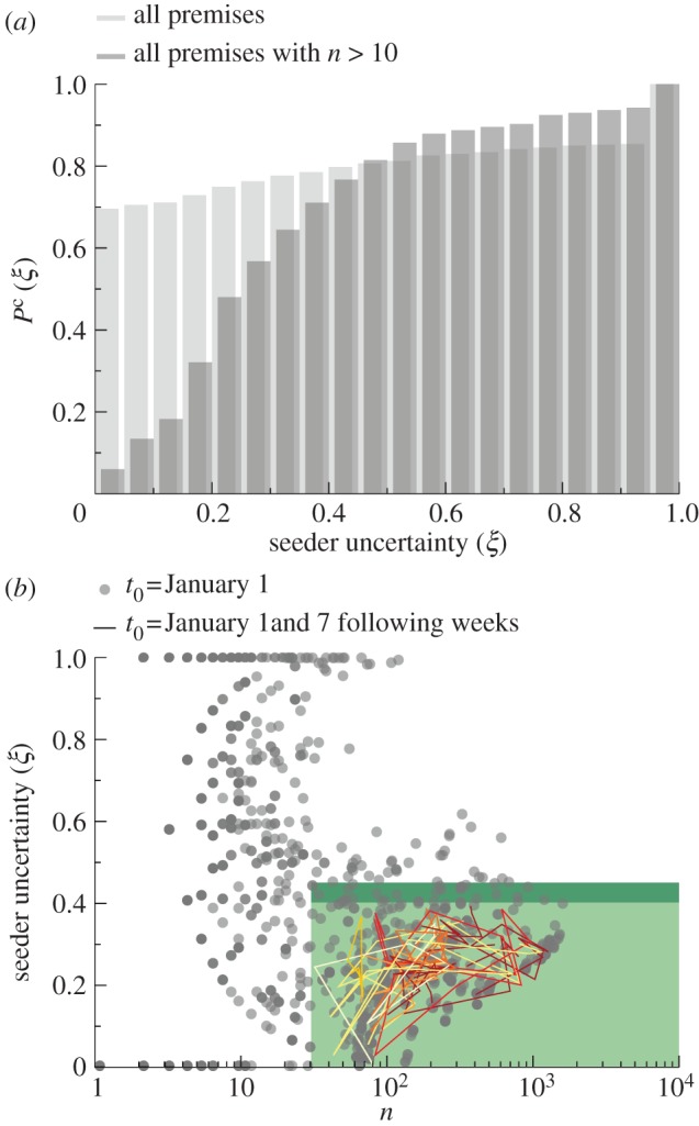
Sentinel premises. (a) Cumulative probability distribution of the uncertainty ξ of a given premises in the identification of the seeding cluster. Slaughterhouses are discarded from the analysis, as they cannot spread the disease further to other farms. (b) For a set of initial conditions with t₀ = 1 January, each infected farm is represented by a dot in the phase space, with n being the number of times the farm is reached by an infection. Sentinel nodes are defined as the farms that are often reached by epidemics (i.e. ) and have a low degree of uncertainty in the identification of the seeding cluster that led to the outbreak (i.e. ). The plot shows the trajectories in the phase space of the 15 sentinels obtained by imposing and , for eight consecutive weeks starting from 1 January.

The uncertainty on the identification of the cluster of initial conditions infecting node k and the number of times n_k node k is reached by the epidemic clearly depend on the time t₀ of the start of the epidemic. In the following, we explore the variation of these two quantities for all nodes of the network when we consider epidemics starting at time t₀ = 1 January +7w with w = 0, 1, 2, 3, … , 8, i.e. spanning an eight-week interval from 1 January. In figure 7b, we represent each farm k as a point with coordinates in the phase space, for t₀ = 1 January. As t₀ changes, a variety of different behaviours is obtained, as expected given the large variability of the network. Large fluctuations of the number of times a node is infected are observed, as a node with a large n_k (i.e. often reached by the disease) for an initial time t₀ may be rarely reached if the outbreak starts later, given the change in the network of displacements, or may even disappear from the plot if it is not infected for a given explored initial time (i.e. it has n_k = 0). Similarly, also the values of the uncertainty in the identification of the seeding cluster can strongly fluctuate. From the surveillance perspective, we are interested in the nodes that are infected a large number of times (i.e. are probably reached by the epidemic, given any temporal and geographical initial conditions) and for which we have a low uncertainty in the identification of the seeding cluster, providing important insights into previous and future spreading patterns. We define these premises as sentinel nodes by imposing that they are infected at least times and are characterized by an uncertainty at most equal to for all initial conditions. Their trajectories in the phase space for varying t₀ are shown in figure 7b for and . The choice of the threshold values depends on the resources available to monitor these sentinels: smaller and larger lead to a larger number of sentinels. In the electronic supplementary material, table S1, we report the number of sentinels for different values. It is also possible to be less conservative and enlarge the group of possible sentinels for efficient detection of an infectious disease by including farms with discontinuous trajectories that may have n_k = 0 for one value of the starting time but have and for the other starting times. By relaxing these constraints, it is possible to build a hierarchy of disease sentinels with different levels of reliability, and specific to the available surveillance resources. In the electronic supplementary material, we also tested an alternative definition of the entropy function showing that it does not alter the results.

The interest of the definition of sentinel nodes in the perspective of a surveillance system is quantified further in figure 8a. Given a set of sentinels, we measure the fraction of detected outbreaks as a function of the outbreak final size, where an outbreak is considered detected if it infects at least a sentinel farm. Figure 8a shows that sentinels are not good indicators for the presence of small outbreaks (i.e. corresponding to sizes smaller than 5–10 infected farms); however, a surveillance system based on only 15 sentinel nodes (out of a total number of more than 170 000 premises) would detect more than 55 per cent of the outbreaks with final size being larger than 10 and, if the number of sentinels is increased to 32, the fraction of outbreaks detected would be more than 75 per cent. Finally, it is also important to consider that the information provided by the sentinel farms is meaningful as long as the detection occurs rather early in the outbreak evolution. We evaluated the rapidity of detection by plotting the infection time of each of the 15 sentinel farms (obtained with and ) relative to the full outbreak duration, for outbreaks of size larger than 10 (figure 8b). Interestingly, almost all sentinels are able to detect most outbreaks within the first third of the outbreak duration. Similar results are also valid for the stochastic case, as reported in the electronic supplementary material.

Figure 8.

Properties of the surveillance system based on sentinel premises. (a) Fraction of outbreaks detected by the sentinels as a function of the minimum outbreak size of the epidemic, for two sets of sentinels (of 15 and 32 sentinels), corresponding to , ) and (, ), respectively. (b) Boxplot of the time of infection of the 15 sentinels relative to the full duration of the outbreak, considering the detected outbreaks with final size being larger than 10. Each box is coloured according to the number of times n that the sentinel has been infected and a grey shaded area indicates 33% of the relative infection time. (c) Topological properties of sentinel nodes (red dots), compared to the other nodes (smaller black dots). All premises in the system (except slaughterhouses) are represented in the plane of the number of in-connection versus the number of out-connections per premises. Sentinels may be characterized by either small or large number of in–out connections. (d) As in (c), but showing the fluxes properties in the plane of the number of batches moved in and out of each premises. Even in this case, sentinels may assume small to large values in the parameter space.

Finally, it is interesting to note how sentinel nodes cannot be identified through geographical, topological or flux analyses only. Figure 8c–d shows the properties of the sentinel nodes in terms of the number of in- and out-connections, and of the number of batches moved in and out of the premises, highlighting how sentinels do not share similar properties and span largely fluctuating values in the parameter space.

4. Discussion

The full knowledge of livestock movements on a daily resolution makes it possible to investigate in detail the spreading patterns of livestock emerging diseases. Through simulations on the fully dynamic network, where daily bovine movements are explicitly captured, we have studied the role of the initial conditions in shaping the propagation process. Clusters of seeds emerge that lead to similar spreading patterns in terms of infected premises, and are also characterized by similar epidemic profiles and peak times. These clusters cannot be identified from purely structural or geographical considerations. The proposed clustering method can be used in order to optimize surveillance systems and define rapid and efficient containment strategies, targeting farms that are at a high risk of being infected and further spread the disease. Although the displacement network is characterized by a large temporal variability, intrinsically altering the centrality role of nodes from a given observation time to another, it is possible to identify sentinel nodes representing premises, which are often reached by the disease and, when detected as infected, are able to provide valuable information on the seeding farms of the outbreak and thus on the likely spreading path, allowing targeted intervention strategies to be designed. A hierarchical classification of sentinels can be provided by tuning the constraints imposed for their definition, leading to different levels of surveillance. Remarkably, the bare knowledge of animal movements would not be enough to estimate the origin of a disease, once detected, as the outbreak results from the complex interplay of the dynamical network and the disease dynamics. On the other hand, this interplay leads to the emergence of a very small number of sentinels, with respect to the total number of premises present in the system, that may be efficiently used for disease prevention and control.

Applications to specific diseases, where the timescale of the epidemic is set by the parameters describing the disease aetiology, can be performed to tune this framework to particular cases. These findings clearly depend on the full knowledge of the displacement dataset, and can thus be obtained as a priori information during a non-emergency period to help orienting control strategies, as commonly done with the static analysis of the contact network structure, strengthening the importance of such data collection. The ability to make useful predictions for current and future livestock movements patterns depends on the level of similarity across different years of data. The analysis of successive years of movement data, uncovering possible recurrent patterns and seasonal behaviours, may thus contribute to make this framework a general tool to be used in real-time emergencies.

References

- 1.Anderson I. 2002. Foot and mouth disease 2001: lessons to be learned inquiry report. London, UK: The Stationary Office [Google Scholar]
- 2.Taylor L. H., Latham S. M., Woolhouse M. E. 2001. Risk factors for human disease emergence. Phil. Trans. R. Soc. Lond. B 356, 983–989 10.1098/rstb.2001.0888 (doi:10.1098/rstb.2001.0888) [DOI] [PMC free article] [PubMed] [Google Scholar]
- 3.Ferguson N. M., Donnelly C. A., Anderson R. M. 2001. The foot-and-mouth epidemic in Great Britain: pattern of spread and impact of interventions. Science 292, 1155–1160 10.1126/science.1061020 (doi:10.1126/science.1061020) [DOI] [PubMed] [Google Scholar]
- 4.Keeling M. J., et al. 2001. Dynamics of the 2001 UK foot and mouth epidemic: stochastic dispersal in a heterogeneous landscape. Science 294, 813–817 10.1126/science.1065973 (doi:10.1126/science.1065973) [DOI] [PubMed] [Google Scholar]
- 5.Kao R. R. 2003. The impact of local heterogeneity on alternative control strategies for foot-and-mouth disease. Proc. R. Soc. Lond. B 270, 2557–2564 10.1098/rspb.2003.2546 (doi:10.1098/rspb.2003.2546) [DOI] [PMC free article] [PubMed] [Google Scholar]
- 6.Keeling M. J. 2005. Models of foot-and-mouth disease. Proc. R Soc. B 272, 1195–1202 10.1098/rspb.2004.3046 (doi:10.1098/rspb.2004.3046) [DOI] [PMC free article] [PubMed] [Google Scholar]
- 7.Carpenter T. E., O'Brien J. M., Hagerman A. D., McCarl B. A. 2011. Epidemic and economic impacts of delayed detection of foot-and-mouth disease: a case study of a simulated outbreak in California. J. Vet. Diagn. Invest. 23, 26–33 10.1177/104063871102300104 (doi:10.1177/104063871102300104) [DOI] [PubMed] [Google Scholar]
- 8.Christley R. M., Robinson S. E., Lysons R., French N. P. 2005. Network analysis of cattle movement in Great Britain. Proc. Soc. Vet. Epidemiol. Prev. Med. 234–243 [Google Scholar]
- 9.Ortiz-Pelaez A., Pfeiffer D. U., Soares-Magalhaes R. J., Guitian F. J. 2006. Use of social network analysis to characterize the pattern of animal movements in the initial phases of the 2001 foot and mouth disease (FMD) epidemic in the UK. Prev. Vet. Med. 76, 40–55 10.1016/j.prevetmed.2006.04.007 (doi:10.1016/j.prevetmed.2006.04.007) [DOI] [PubMed] [Google Scholar]
- 10.Bigras-Poulin M., Thompson R. A., Chriel M., Mortensen S., Greiner M. 2006. Network analysis of Danish cattle industry trade patterns as an evaluation of risk potential for disease spread. Prev. Vet. Med. 76, 11–39 10.1016/j.prevetmed.2006.04.004 (doi:10.1016/j.prevetmed.2006.04.004) [DOI] [PubMed] [Google Scholar]
- 11.Green D. M., Kiss I. Z., Kao R. R. 2006. Modeling the initial spread of the foot-and-mouth disease through animal movements. Proc. R. Soc. B 273, 2729–2735 10.1098/rspb.2006.3648 (doi:10.1098/rspb.2006.3648) [DOI] [PMC free article] [PubMed] [Google Scholar]
- 12.Kao R. R., Danon L., Green D. M., Kiss I. Z. 2006. Demographic structure and pathogen dynamics on the network of livestock movements in Great Britain. Proc. R. Soc. B 273, 1999–2007 10.1098/rspb.2006.3505 (doi:10.1098/rspb.2006.3505) [DOI] [PMC free article] [PubMed] [Google Scholar]
- 13.Robinson S. E., Everett M. G., Christley R. M. 2007. Recent network evolution increases the potential for large epidemics in the British cattle population. J. R. Soc. Interface 4, 669–674 10.1098/rsif.2007.0214 (doi:10.1098/rsif.2007.0214) [DOI] [PMC free article] [PubMed] [Google Scholar]
- 14.Kao R. R., Green D. M., Johnson J., Kiss I. Z. 2007. Disease dynamics over very different time-scales: foot-and-mouth disease and scrapie on the network of livestock movements in the UK. J. R. Soc Interface 4, 907–916 10.1098/rsif.2007.1129 (doi:10.1098/rsif.2007.1129) [DOI] [PMC free article] [PubMed] [Google Scholar]
- 15.Natale F., Giovannini A., Savini L., Palma D., Possenti L., Fiorea G., Calistrib P. 2009. Network analysis of Italian cattle trade patterns and evaluation of risks for potential disease spread. Prev. Vet. Med. 92, 341–350 10.1016/j.prevetmed.2009.08.026 (doi:10.1016/j.prevetmed.2009.08.026) [DOI] [PubMed] [Google Scholar]
- 16.Dube C., Ribble C., Kelton D., McNab B. 2009. A review of networks analysis terminology and its application to foot-and-mouth disease modeling and policy development. Transbound. Emerg. Dis. 56, 73–85 10.1111/j.1865-1682.2008.01064.x (doi:10.1111/j.1865-1682.2008.01064.x) [DOI] [PubMed] [Google Scholar]
- 17.Martinez-Lopez B., Perez A. M., Sanchez-Vizcaino J. M. 2009. Social network analysis. Review of general concepts and use in preventive veterinary medicine. Transbound. Emerg. Dis. 56, 109–120 10.1111/j.1865-1682.2009.01073.x (doi:10.1111/j.1865-1682.2009.01073.x) [DOI] [PubMed] [Google Scholar]
- 18.Vernon M. C., Keeling M. J. 2009. Representing the UK's cattle herd as static and dynamic networks. Proc. R. Soc. B 276, 469–476 10.1098/rspb.2008.1009 (doi:10.1098/rspb.2008.1009) [DOI] [PMC free article] [PubMed] [Google Scholar]
- 19.Volkova V. V., Howey R., Savill N. J., Woolhouse M. E. J. 2010. Potential for transmission of infections in networks of cattle farms. Epidemics 2, 116–122 10.1016/j.epidem.2010.05.004 (doi:10.1016/j.epidem.2010.05.004) [DOI] [PubMed] [Google Scholar]
- 20.Rautureau S., Dufor B., Durand B. 2010. Vulnerability of animal trade networks to the spread of infectious diseases: a methodological approach applied to evaluation and emergency control strategies in cattle, France, 2005. Transbound. Emerg. Dis. 10.1111/j.1865-1682.2010.01187 (doi:10.1111/j.1865-1682.2010.01187). [DOI] [PubMed] [Google Scholar]
- 21.Natale F., Savini L., Giovannini A., Calistri P., Candeloro L., Fiore G. 2011. Evaluation of risk and vulnerability using a disease flow centrality measure in dynamic cattle trade networks. Prev. Vet. Med. 98, 111–118 10.1016/j.prevetmed.2010.11.013 (doi:10.1016/j.prevetmed.2010.11.013) [DOI] [PubMed] [Google Scholar]
- 22.Bajardi P., Barrat A., Natale F., Savini L., Colizza V. 2011. Dynamical patterns of cattle trade movements. PLoS ONE 6, e19869 10.1371/journal.pone.0019869 (doi:10.1371/journal.pone.0019869) [DOI] [PMC free article] [PubMed] [Google Scholar]
- 23.Barabasi A.-L., Albert R. 1999. Emergence of scaling in random networks. Science 286, 509–512 10.1126/science.286.5439.509 (doi:10.1126/science.286.5439.509) [DOI] [PubMed] [Google Scholar]
- 24.Dorogovstev S. N., Mendes J. F. F. 2003. Evolution of networks: from biological nets to the internet and WWW. Oxford, UK: Oxford University Press [Google Scholar]
- 25.Newman M. E. J. 2003. The structure and function of complex networks. SIAM Rev. 45, 167 10.1137/S003614450342480 (doi:10.1137/S003614450342480) [DOI] [Google Scholar]
- 26.Barrat A., Barthélemy M., Vespignani A. 2008. Dynamical processes on complex networks. Cambridge, UK: Cambridge University Press; 10.1017/CBO9780511791383 (doi:10.1017/CBO9780511791383) [DOI] [Google Scholar]
- 27.Friedkin N. E. 1991. Theoretical foundations for centrality measures. Am. J. Sociol. 96, 1478–1504 10.1086/229694 (doi:10.1086/229694) [DOI] [Google Scholar]
- 28.Albert R., Jeong H., Barabasi A.-L. 2000. Error and attack tolerance of complex networks. Nature 406, 378–482 10.1038/35019019 (doi:10.1038/35019019) [DOI] [PubMed] [Google Scholar]
- 29.Cohen R., Erez K., ben-Avraham D., Havlin S. 2001. Breakdown of the Internet under intentional attack. Phys. Rev. Lett. 86, 3682–3685 10.1103/PhysRevLett.86.3682 (doi:10.1103/PhysRevLett.86.3682) [DOI] [PubMed] [Google Scholar]
- 30.Pastor-Satorras R., Vespignani A. 2001. Epidemic spreading in scale-free networks Phys. Rev. Lett. 86, 3200–3203 10.1103/PhysRevLett.86.3200 (doi:10.1103/PhysRevLett.86.3200) [DOI] [PubMed] [Google Scholar]
- 31.Lloyd A., May R. 2001. Epidemiology: how viruses spread among computers and people. Science 292, 1316–1317 10.1126/science.1061076 (doi:10.1126/science.1061076) [DOI] [PubMed] [Google Scholar]
- 32.Kitsak M., Gallos L. K., Havlin S., Liljeros F., Muchnik L., Eugene Stanley H., Makse H. A. 2010. Identification of influential spreaders in complex networks. Nat. Phys. 8, 888–893 10.1038/nphys1746 (doi:10.1038/nphys1746) [DOI] [Google Scholar]
- 33.Woolhouse M. E., Shaw D. J., Matthews L., Liu W. C., Mellor D. J., Thomas M. R. 2005. Epidemiological implications of the contact network structure for cattle farms and the 20–80 rule. Biol. Lett. 1, 350–352 10.1098/rsbl.2005.0331 (doi:10.1098/rsbl.2005.0331) [DOI] [PMC free article] [PubMed] [Google Scholar]
- 34.Brennan M. L., Kemp R., Christley R. M. 2008. Direct and indirect contacts between cattle farms in north-west England. Prev. Vet. Med. 84: 242–260 10.1016/j.prevetmed.2007.12.009 (doi:10.1016/j.prevetmed.2007.12.009) [DOI] [PubMed] [Google Scholar]
- 35.Keeling M. J., Danon L., Vernon M. C., House T. A. 2010. Individual identity and movement networks for disease metapopulations. Proc. Natl Acad. Sci. USA 107, 8866–8870 10.1073/pnas.1000416107 (doi:10.1073/pnas.1000416107) [DOI] [PMC free article] [PubMed] [Google Scholar]
- 36.Anderson R. M., May R. M. 1992. Infectious diseases of humans: dynamics and control. Oxford, UK: Oxford University Press [Google Scholar]
- 37.Kostakos V. 2009. Temporal graphs. Phys. A 388, 1007–1023 10.1016/j.physa.2008.11.021 (doi:10.1016/j.physa.2008.11.021) [DOI] [Google Scholar]