Universal Algorithm for Identification of Fractional Brownian Motion. A Case of Telomere Subdiffusion

Abstract

We present a systematic statistical analysis of the recently measured individual trajectories of fluorescently labeled telomeres in the nucleus of living human cells. The experiments were performed in the U2OS cancer cell line. We propose an algorithm for identification of the telomere motion. By expanding the previously published data set, we are able to explore the dynamics in six time orders, a task not possible earlier. As a result, we establish a rigorous mathematical characterization of the stochastic process and identify the basic mathematical mechanisms behind the telomere motion. We find that the increments of the motion are stationary, Gaussian, ergodic, and even more chaotic—mixing. Moreover, the obtained memory parameter estimates, as well as the ensemble average mean square displacement reveal subdiffusive behavior at all time spans. All these findings statistically prove a fractional Brownian motion for the telomere trajectories, which is confirmed by a generalized p-variation test. Taking into account the biophysical nature of telomeres as monomers in the chromatin chain, we suggest polymer dynamics as a sufficient framework for their motion with no influence of other models. In addition, these results shed light on other studies of telomere motion and the alternative telomere lengthening mechanism. We hope that identification of these mechanisms will allow the development of a proper physical and biological model for telomere subdynamics. This array of tests can be easily implemented to other data sets to enable quick and accurate analysis of their statistical characteristics.

Introduction

Our work is motivated from one side by the growing interest in single molecule spectroscopy (1–16), in particular by single-particle tracking (SPT) in a context of anomalous diffusion (11,18–25) and from the other side by the discovery of how chromosomes are protected by telomeres and the enzyme telomerase (26). By performing a thorough statistical analysis on a very large data set of telomere motions, we set new perspectives, to our knowledge, on telomere dynamics and show how to systematically analyze future SPT results.

SPT measurements can provide new experimental knowledge even with basic analysis. For example, diffusion coefficients and qualitative behavior of the measured species can be found by analyzing the mean square displacement $\langle x^2\left(t\right)\rangle$ (MSD). However, there is much more to be obtained if one dives deeper into the statistical nature of the data, possibly even contradicting the results of simpler analysis. In the case of anomalous diffusion, i.e., when the MSD is not linear in t, the importance of thorough analysis is intensified as there are many mathematical and physical models that can give rise to similar forms of MSDs (27). A recent example of the strength of stochastic analysis is the study of the dynamics of Kv2.1 potassium channels in cellular membranes (28) that showed compartmentalization and binding.

A phenomenon observed in recent nanoscale single-molecule biophysics experiments is subdiffusion, which largely departs from the classical Brownian diffusion theory. Determining the origin anomalous diffusion in crowded fluids, e.g., in the cytoplasm of living cells (29), or in more controlled in vitro experiments (9), is a challenging problem. The most popular theoretical models that are commonly employed are continuous-time random walk (CTRW), obstructed diffusion (OD), fractional Brownian motion (FBM), fractional Levy stable motion (FLSM), and fractional Langevin equation (FLE) (30–40). These models can be divided into two categories: with short memory (CTRW, OD) and fractional with long (power law) memory (FBM, FLSM, FLE, and fractional autoregressive moving average (FARIMA)). The FARIMA model unifies the latter category (31).

To date, there is no standard analysis scheme that can identify the mathematical model behind a wide variety of measured anomalous trajectories. Each of these models has a unique definition, which implies unique characteristics and thus various tests have been proposed to differentiate between them (35–39). However, each of these tests covers only a limited set of characteristics, and hence does not capture the complete stochastic picture. It is therefore expected that a standardized testing scheme for different models that would encompass a variety of different experimental scenarios would be highly beneficial.

FBM statistically behaves identical to FLE in the overdamped limit. However, the noise in FBM is external and not coupled to fluctuations, in contrast to the FLE motion, for which a proper temperature is defined (40). FBM/FLE motion is the effective motion of a labeled, single particle connected with a many-particle system, such as a monomer in a long polymer, or an individual particle in a single file (41).

One system that was suggested to obey such fractional dynamics is the motion of telomeres in the eukaryotic nucleus (42). Telomeres form the capping structures at the ends of each chromosome. They consist of a repeating DNA sequence and a specific protein complex surrounding it (named shelterin). The telomeres play an important role in maintaining the chromosomal integrity, preventing adhesion of chromosomes to one another, as well as degradation of the ends of the chromosomes through enzymes that are abundant in the nucleus (43–45). The telomeres lose a short piece of the DNA each time the chromosome is replicated. This shortening is believed to be related to aging, although the actual mechanisms are much more complex (46).

Because there are a significant number of telomeres (92 in humans) that are, generally speaking, uniformly distributed in the nucleus, they form excellent probes for investigating the dynamics of the DNA and its accompanying proteins called chromatin. The telomeres can be labeled in living cells through one of the native shelterin proteins using fluorescent proteins such as the green fluorescent protein. The first publication of telomeres diffusion appeared in (47).

During the last few years, the dynamics of telomeres was studied more carefully by analyzing their diffusion properties. This method can provide important information on the structure and function of the chromatin in general, and the telomeres themselves in particular. Previous study has found the telomeres motion to be subdiffusive up to 10² s with an anomalous exponent of $\alpha =0.32\pm 0.12-0.51\pm 0.20$ and a higher anomalous exponent at longer times (48). Because anomalous diffusion can originate from various mechanisms (19,27), further analysis can shed light on the nuclear mechanisms behind telomere motion. Thus, a better picture of in vivo chromatin motion and nuclear structure can be obtained.

A follow-up analysis of short time motion of telomeres proved (42) that binding and CTRW models are not the origin of the subdiffusive regime. Displacements were found to be correlated in time and weak ergodicity convergence complied with the prediction for fractional processes. Thus, it was proposed that some correlative mechanism stands behind the local motion of chromatin and telomeres, specifically throughout the interphase. In this study, the possibility that the anomalous diffusion of telomeres stems from obstruction of motion in the nucleus by quasistatic obstacles was also looked into and found inadequate.

In parallel, a series of studies have connected telomere motion to their elongation and maintenance. This was proposed for telomerase-positive cancer cells (UMUC3) (49) and for U2OS cancer cells that use the alternative lengthening of telomeres (ALT) mechanism (50). In both cases, heterogeneity of the telomere population was claimed. It was proposed that this heterogeneity enables a motion-based control mechanism for telomere elongation. Recently, another study (51) showed that transcription activity also influences telomere motion.

In this work, we first present a universal, systematic, and intuitive algorithm for the identification and validation of FBM. The proposed algorithm tests all the fundamental characteristics of FBM. In addition, ergodicity is also tested for and its significance in the context of data analysis explained. Furthermore, the important property of the self-similarity of the process is validated with two independent tests. Compliance with the testing scheme given here proves that FBM is the only mathematical model suitable for the data tested.

To prove the ability of the proposed algorithms to test various data structures, we analyze an expanded version of the data presented in (48). The data are divided into three time domains, each with a different measurement rate and amount of trajectories. The telomere motion is found to follow the FBM process in over five time orders, a conclusion not possible with previous analysis. This, to our knowledge, sheds new light on the motion of telomeres measured in the previously mentioned works and on chromatin dynamics in general.

Methods

Experimental methodology

A full description of the experimental procedure is given in the Supporting Material and in (48). In short, telomeres in U2OS osteosarcoma cells are labeled with a protein composed of a green fluorescent protein attached to a TRF-1 protein. Cells are then imaged from millisecond time frames and up to 30 min. Images are analyzed for telomere tracks with the use of Imaris and Image J software. Tracks are then analyzed for stochastic traits with in-house written scripts and programs.

The experimental noise was measured by measuring telomere motion after fixating the cells. It was found that the effective noise in all timescales is Gaussian with zero mean and a variance of 22 nm. For more details see the Supporting Material.

Identification and validation algorithm

It is natural to expect a universal identification algorithm for FBM that would encompass a variety of different experimental scenarios. Such an algorithm would give rise to confidence levels of results and enable benchmarking between different experiments and systems. Ultimately such an algorithm would direct the experimental process because it would indicate which tests should be applied to the analyzed data.

What are the requirements for such an algorithm? First of all, it should be applicable to any trajectory data, i.e., it should be universal. An SPT data structure is composed of independent trajectories for single particles, measured at a certain frame rate. Each trajectory can be in a single dimension or more. Both the number of trajectories and the amount of data points may vary between data sets. A good algorithm should work sufficiently well both in the case of many trajectories with a few data points or a few trajectories with many data points.

Second, such an algorithm should be systematic. It should identify all fundamental characteristics of a certain mathematical model. When looking at a single characteristic, it is possible to eliminate a certain model but not to validate one. However, if all fundamental characteristics of a model are verified, we can then confirm that the measured process is indeed of that type. Erroneous results have been known to arise when not all assumptions of a stochastic model have been tested for (52).

Finally, any algorithm should be easy to implement and its conclusions clear. This implies that one should be able to derive a valid biophysical conclusion about the process even without diving into all the subtle mathematical details of the tests.

Following, we propose such a complete algorithm for the identification and validation of the FBM process. Each step requires only standard data found in any SPT measurement. Some steps use the results of the previous steps to reach accurate conclusions. Hence, conclusions of a single test should be drawn in compliance with the previous steps. Upon completion of all steps, one can reach a conclusion as of the nature of the measured process with the ability to assess the error bounds of the results.

Fractional Brownian motion identification and validation algorithm

• •Check stationarity of the data using the quantile lines test—parallel for increments of FBM.
• •Verify probability distribution of the increments using Jarque-Bera (JB), Kolmogorov-Smirnov (KS), Anderson-Darling (AD), Cramer-von Mises (CM), and Kuiper (K) tests—Gaussian for FBM.
• •Check ergodicity behavior of the data with the dynamical functional test—ergodic and mixing for increments of FBM.
• •Find the self-similarity parameter H and memory parameter d from the sample and ensemble average MSD using the Boltzmann ergodic hypothesis. FBM has a negative d and $H<0.5$.
• •Validate the subdiffusion model of motion and self-similarity parameter H with the generalized p-variation test.

A detailed description of the consecutive steps of the algorithm will be given in the Results section.

From a statistical point of view, experimental noise does not affect crucial properties of the underlying process like self-similarity and type of diffusion. The tests we present will give the correct nature of the process as long as the added noise is not of a much larger magnitude than the true process, which is true in our experiment, see Figs. S1–S3 in the Supporting Material.

For the identification of the memory parameter, it has been shown (53) that noise can lower the apparent MSD exponent. However, this will only change the exact value of parameters found and not the stochastic nature of the data.

Results

We analyze data recorded in three time regimes related to three different measurement methods: 10⁻² − 10 [s] (CCD), 1 − 10² [s] (2D confocal), and 10 − 10³ [s] (3D confocal), Fig 1. X and Y coordinates are studied separately. We show that the telomere trajectories have stationary, Gaussian, ergodic, and even mixing increments. Both the time average and ensemble average MSD reveal subdiffusive behavior. All the analyses lead to the conclusion that the telomere motion can be described by a FBM. This is strengthened by the generalized p-variation test, which clearly shows the self-similar nature of the data and together with the results of ergodicity rejects the CTRW hypothesis.

Figure 1.

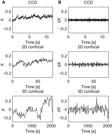
Sample trajectories of X time series (A) and of their increments (B) corresponding to each of the time regimes: CCD (top panel), 2D (middle panel), 3D (bottom panel).

Stationarity and probability distribution

As mentioned previously, stationarity of the process or its increments is a fundamental characteristic of a stochastic process. Hence, we start with verifying the stationarity property of the analyzed data sets. We plot the quantile lines, see Fig. 2, a standard test for stationarity (54), calculated from the analyzed trajectories. Let us assume that we observe M samples of length N and denote their values by $\left\{Z_n^k\right\}$, $n=1,2,\dots N$, $k=1,\dots ,M$, and $0<p_j<1$, $j=1,\dots ,J$ are given probabilities. It is possible to derive estimators of the corresponding quantiles $q_j\left(n\right)=F_n^{-1}\left(p_j\right)$, where $F_n=F_n\left(x\right)$ denotes the unknown cumulative distribution function of the random variable $Z_n$ represented by the statistical sample $Z_n^k$, $k=1,\dots ,M$. In this way we obtain the approximation of the so-called quantile lines, i.e., the curves

$$q_j=q_j\left(n\right),$$

defined by the condition

$$P\left\{Z_n\le q_j\left(n\right)\right\}=p_j.$$ (1)

In layman terms, the quantile lines represent the value $q_j$ for which $p_j\times 100\text{\%}$ of the data are below at a certain time point n. For a stationary process the quantile lines $q_j\left(n\right)=\text{const}$, whereas for a self-similar process they behave like $n^H$ (55).

Figure 2.

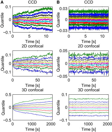
Quantile lines of X trajectories (A) and of their increments (B) corresponding to each of the time regimes: CCD (top panel), 2D confocal (middle panel), 3D confocal (bottom panel). The shape of the quantile lines shows the self-similar (A) and stationary (B) behaviors.

Observe that the obtained curves are not parallel and resemble a power function, see Fig. 2 A, which indicates nonstationarity and self-similarity. On the other hand, quantile lines obtained for the increments of the process are parallel (see Fig. 2 B), therefore the stationarity hypothesis for the increments cannot be rejected. The increments are defined as $d{X}_n=X_{n+1}-X_n$ and $d{Y}_n=Y_{n+1}-Y_n$. Sample time series of $d{X}_n$ are plotted in Fig. 1 B. Observe that each time series corresponds to one trajectory from Fig. 1 A.

Another important characteristic of a stochastic motion is Gaussianity, required, for example, in the case of FBM. To assess the Gaussianity of the increments we analyze the probability density functions (PDFs). In Fig. 3 A we plot PDF of $dX$ time series, which are estimated using the kernel density method (54). Each panel consists of 20 PDFs calculated for sample trajectories recorded within the corresponding time regime. The obtained curves resemble a Gaussian PDF, but the standard deviation of the distribution differs for different trajectories and time regimes (observe different scales in panels of Fig. 3 A).

Figure 3.

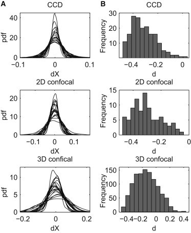
Probability density functions of dX time series (A) and histograms of the memory parameter d obtained for X time series (B) corresponding to each of the time regimes: CCD (top panel), 2D confocal (middle panel), 3D confocal (bottom panel).

To confirm a visual observation that the increments of the analyzed data sets are Gaussian, we perform statistical goodness-of-fit tests on all telomere trajectories in both X and Y. Precisely, we conduct the JB, KS, AD, CM, and K tests (56,57). In Table 1 we provide percentages of the trajectories for which we can reject (at the 5% significance level) a hypothesis that the increments follow the Gaussian law.

Table 1.

Percentage of trajectories for which we can reject (at the 5% significance level) a hypothesis that the increments follow the Gaussian law

Test	CCD		2D confocal		3D confocal
	dX	dY	dX	dY	dX	dY
JB	5.5%	7.2%	4.3%	3.2%	10.6%	11.3%
KS	5.5%	5.5%	5.4%	6.5%	6.1%	6.9%
AD	4.4%	6.7%	5.4%	4.3%	6.4%	7.1%
CM	2.8%	6.1%	5.4%	4.3%	6.0%	6.8%
K	3.9%	5.5%	7.5%	6.5%	5.6%	7.0%

Observe that in almost all cases percentage of the trajectories with rejected normality of increments is close to the significance level, i.e., 5%. Hence, we can conclude that the motion of telomere can be described by Gaussian increments.

Ergodicity and mixing

Next, we will study another two fundamental properties of the data: ergodicity and mixing. Ergodicity of the stationary process $Z\left(n\right)$ means that its phase space cannot be divided into two nontrivial sets such that a point starting in one set will never get to the second set. Let us emphasize that for every stationary and ergodic process the Boltzmann ergodic hypothesis, enabling better analysis of the data characteristics is satisfied, i.e., the temporal and ensemble averages coincide (58,59).

Another fundamental property is mixing, i.e., the asymptotic independence of the random variables $Z\left(n\right)$ and $Z\left(0\right)$ as n goes to infinity. It is well known that mixing is a stronger property than ergodicity (60). Thus, to show ergodicity it is enough to prove mixing, which is easier in many cases.

To this end, we use the dynamical functional (DF) test recently developed in (61). It is based on a concept of the dynamical functional (54)

$$D\left(n\right)=\langle \text{exp}\left\{i\left(Z\left(n\right)-Z\left(0\right)\right)\right\}\rangle .$$ (2)

Note that $D\left(n\right)$ is actually a Fourier transform of the process increment evaluated for the Fourier-space variable $k=1$. Denote by $E\left(n\right)=D\left(n\right)-{\left|\langle \text{exp}\left\{iZ\left(0\right)\right\}\rangle \right|}^2$. It turns out that stationary process $Z\left(n\right)$ is mixing if and only if

$$\underset{n\to \mathrm{\infty }}{\text{lim}}E\left(n\right)=0.$$ (3)

Similarly, $Z\left(n\right)$ is ergodic if and only if

$$\underset{n\to \mathrm{\infty }}{\text{lim}}\frac{1}{n}\sum _{k=0}^{n-1}E\left(k\right)=0.$$ (4)

The DF test holds for all infinitely divisible stationary processes (61,62). Because telomere data have stationary and Gaussian increments we can apply it. In Fig. S5 A we show the ergodicity test results (calculated as the ensemble average over all trajectories within a certain time range), whereas in Fig. S5 B the mixing test results. Note, the test indicates ergodicity (or mixing, respectively) if the plotted curves converge to zero.

The DF test confirms that the increments of telomere motion have the ergodicity (and mixing) property. Because such properties are also valid for the increments of FBM, we cannot reject FBM as a proper model for the analyzed data. Analogous results are obtained for the Y coordinate. This result allows us to reject a CTRW model for the motion. Furthermore, according to the Boltzmann ergodic hypothesis we can now use either the time-averaged or the ensemble-averaged results of any analysis according to our preference (61,62). We also note that the weak ergodicity convergence was already checked in (42).

Memory parameter

A necessary property of fractional processes is the correlation of the increments in time. Usually this correlation takes the form of a power law. In what follows, we analyze the memory property of the considered telomere motion. Using the time average mean square displacement we calculate the memory parameter d.

Let $\left\{Z_i,i=1,\dots ,N\right\}$ be a sample of length N. The sample MSD was introduced in (63). as

$$M_N\left(\tau \right)=\frac{1}{N-\tau }\sum _{k=1}^{N-\tau }{\left(Z_{k+\tau }-Z_k\right)}^2.$$ (5)

The sample MSD is a time average MSD on a finite sample regarded as a function of difference τ between observations. It is a random variable in contrast to the ensemble average, which is deterministic.

If the sample comes from an H-self-similar process with stationary increments belonging to the domain of attraction of the Lévy α-stable law, then for large N

$$M_N\left(\tau \right)\sim {\tau }^{2d+1}{S}_{\alpha /2},$$ (6)

where ∼ means similarity in distribution, $d=H-1/\alpha$, and $S_{\alpha /2}$ is a totally skewed $\alpha /2$ -stable random variable (56,63).

If $\alpha =2$, i.e., we have a Gaussian law or data with finite second moment, then for large N and small τ $M_N\left(\tau \right)\sim {\tau }^{2d+1}\langle Z_1^2\rangle ,$ where $d=H-1/2$. In particular, for a FBM we obtain the well-known result that $M_N\left(\tau \right)\sim {\tau }^{2H}$, and for a Brownian motion we arrive at the diffusion case, namely $M_N\left(\tau \right)\sim \tau$ since $d=0$, see also (64).

As a consequence, we see that the memory parameter d controls the type of anomalous diffusion. If $d<0$ $\left(H<1/2\right)$, therefore in the negative dependence case, the process follows the subdiffusive dynamics, if $d>0$ $\left(H>1/2\right)$, the character of the process changes to superdiffusive. The subdiffusion pattern arises when the dependence is negative; therefore, positive increments are quickly compensated by the negative.

In Table 2 we present the means and standard deviations (STDs) of the anomalous exponent $a=2d+1$ and memory parameter d estimates obtained for each coordinate and each time range. For the CCD and 2D confocal measurement data sets we obtain a strong evidence for the negative memory, as the mean of the obtained d estimates is around –0.35 and the STD does not exceed 0.09. For the 3D confocal measurements the mean of the memory parameter estimates is higher (around –0.18) and the STD of the estimates is larger (up to 0.15), but still the obtained values indicate a negative memory. Looking at the histogram of d in the 3D confocal case (see Fig. 3 B) we may see that values obtained for some of the trajectories are higher than 0. However, we have to remember that the accuracy of the estimates is the lowest for the 3D confocal measurements, because we have only 100 time points. Histograms of the values of d parameter obtained for X trajectories are plotted in Fig. 3 B. We note that the analysis of the Y coordinate yields similar results.

Table 2.

Means, standard deviations, and 95% confidence intervals $\left(\left(C{B}_{2.5\text{\%}},C{B}_{97.5\text{\%}}\right)\right)$ of the MSD exponent, where CB denotes the confidence bound, memory parameter d and the self-similarity parameter H estimates obtained for different time ranges

	CCD		2D		3D
	X	Y	X	Y	X	Y
MSD exponent a = 2d + 1
Mean	0.37	0.36	0.40	0.43	0.71	0.71
STD	0.20	0.18	0.20	0.23	0.33	0.34
$C{B}_{2.5\text{\%}}$	0.08	0.09	0.07	0.10	0.14	0.15
$C{B}_{97.5\text{\%}}$	0.83	0.77	0.82	1.09	1.35	1.39
Memory parameter d
Mean	−0.31	−0.32	−0.30	−0.28	−0.14	−0.15
STD	0.10	0.09	0.08	0.12	0.17	0.17
$C{B}_{2.5\text{\%}}$	−0.48	−0.45	−0.46	−0.45	−0.43	−0.42
$C{B}_{97.5\text{\%}}$	−0.08	−0.12	−0.09	0.04	0.18	0.19
Self-similarity parameter H
Mean	0.18	0.18	0.20	0.21	0.35	0.35
STD	0.10	0.09	0.10	0.11	0.17	0.17
$C{B}_{2.5\text{\%}}$	0.04	0.05	0.03	0.05	0.07	0.08
$C{B}_{97.5\text{\%}}$	0.42	0.38	0.41	0.54	0.68	0.69

Having calculated the memory parameter, we can derive the self-similarity index H, using the relation $d=H-1/2$ because the increments follow the Gaussian distribution, see Table 1. The obtained mean value of H is given in Table 2. Additionally, we provide the STD, as well as the 95% confidence intervals.

Ensemble average MSD

We also investigated the ensemble average MSD. The values of MSD/t obtained for X trajectories are plotted in Fig. 4. Additionally, we plot the fitted power-law function. The anomalous exponent a ranges from 0.47 for the CCD data up to 0.81 for the 3D confocal measurements, indicating a subdiffusive behavior. Similar results can be obtained for the Y coordinate, with the power-law exponent from 0.49 for the CCD data up to 0.9 for the 3D confocal measurements. Thus, we can see that the average parameters in the long time domain are higher than obtained from the time average MSD, but are still anomalous.

Figure 4.

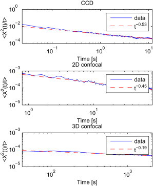
$\langle X^2\left(t\right)/t\rangle$ calculated as the ensemble average (solid lines) together with fitted power law functions (dashed lines). Each panel corresponds to one of the time regimes: CCD (top panel), 2D confocal (middle panel), 3D confocal (bottom panel).

p-Variation

To validate the results on the self-similarity index H, let us now recall the idea of p-variation (38,63,65). Let $Z\left(t\right)$ be a stochastic process analyzed on the time interval $\left[0,T\right]$. The p-variation of $Z\left(t\right)$ is then defined as the limit of sum of increments of $Z\left(t\right)$ taken to the pth power over all partitions of the interval $\left[0,T\right]$, when the mesh of the partitions goes to zero. When $p=1$, it reduces to the total variation, whereas $p=2$ leads to the notion of quadratic variation.

In practice, having a sample of length $N+1$: $\left\{Z_i,i=0,\dots ,N\right\}$, one calculates sample p-variation taking differences between every mth element of the data:

$$V_m^{\left(p\right)}=\sum _{k=0}^{N/m-1}{\left|Z_{\left(k+1\right)m}-Z_{km}\right|}^p.$$ (7)

We plotted in Figs. S6–S8 sample p-variation with respect to m for $p=1/H$, where $H=0.1,0.2,..,0.9$ for the three sample trajectories depicted in Fig. 1. We can see that the behavior of the p-variation in Fig. S6 and Fig. S7 is similar to that of FBM and not of FLSM and CTRW. Namely, the functions show an increasing trend for $p>1/0.2$ (equivalently, for small H), become flat around the value $p=1/0.2$, and for $p<1/0.2$ they result in decreasing functions. This also indicates that the self-similarity index $H\sim 0.2$. The situation in Fig. S8 is not so evident. The decreasing trend for $p<1/0.35$ is visible; however, for small p’s the behavior is quite chaotic. Hence, we cannot draw definite conclusions for this trajectory except for the data being not a CTRW and $H=0.35$. However, we have to remember that the length of this sample is short, only 100 observations. A detailed description of the test based on p-variation is given in the Supporting Material. Finally, observe perfect agreement of the p-variation test with H-self-similarity parameter estimates presented for all three data sets in Table 2.

Discussion

We have presented a universal, systematic, and intuitive algorithm for the identification and validation of FBM. The algorithm implements various tests in a novel, to our knowledge, combination with each test proving a different fundamental characteristic of the process. Gaussianity is confirmed using statistical goodness-of-fit tests. The stationary nature of the incremental process is tested with the use of quantile lines. Finally, self-similarity is deduced from the MSD anomalous exponent, based on the Gaussian nature of the data. In addition, it is shown how to verify these characteristics with the use of other independent tests.

In this work, analysis was performed on the motion of telomeres within six time orders. However, the data are split into three partially overlapping time domains, with a significant difference in experimental character. This is most obvious when comparing the short time measurements, which include 1000 data points to the long time measurements that include only 100 data points. It was shown that the algorithm works well and leads to similar conclusions for all three time domains despite their different structure.

A priori, it was not possible to analyze together the time average results of the short time domain with the ensemble average results of the long time domain. A good example for this is the ergodicity breaking of CTRW, where one will see a different behavior of time and ensemble average observables. This issue is dealt with by proving that our data are stationary and ergodic. Thus, the Boltzmann ergodic hypothesis holds and the two averaging schemes can be analyzed jointly to receive more rigid conclusions about the process.

Our main experimental findings are as follows. Telomere motion increments are shown to be stationary, Gaussian, nonMarkov, and negatively correlated. We remind that for a Brownian motion the increments are stationary, Gaussian, Markov, and independent, i.e., uncorrelated. This characterization enables us to identify the mathematical framework of the process as the FBM. Such a characterization would not have been possible without the use of the complete analysis algorithm. We emphasize that FBM is shown to be the only possible statistical model for telomere motion in all time spans studied.

Two relevant models that show fractional dynamics are the monomer motion polymer systems (66) and diffusion in viscoelastic media like the nucleus (34,67,68). Telomeres are the end monomers of the chromatin chain. We have found that the only statistical model that describes telomere motion is FBM. We identify the biophysical mechanism behind the motion as a thermally driven motion under the constraints of the connected polymer chain (the chromosome) and the nuclear viscoelastic medium. This is in agreement with other recent reports (34,69). This means that no other mechanism such as trapping or obstruction is necessary to explain the characteristics of telomere motion. More than this, from a dynamics point of view, such mechanisms probably do not play a central role in the system. Identification of the viscoelastic modulus and the parameters of the polymer melt are left for future work as is the comparison to other studies on nuclear diffusion (70).

Another polymeric system analyzed lately is that of protein fluctuations (40,71), shown to emerge from the fractal structure of proteins. Although chromatin and proteins are very different in nature (for example, proteins have a stable folding compared to dynamic folding of chromatin), it is interesting to hypothesize that there are underlying structural and dynamical similarities between these two systems.

Our results also shed light on past scientific results. In several past studies (49–51), the anomalous subdiffusive motion of telomeres was not considered. This may be the origin of the decrease in the diffusion coefficient observed in (50) and perhaps of other experimental observations. Furthermore, it was proposed in these studies that differences in the motion between telomeres acted as a control for the telomerase and ALT process. However, ergodic motion, proved with the DF test, implies that the phase space of telomere dynamics cannot be divided into separate subspaces. Hence, the total population of telomeres in U2OS cells (that use the ALT) is not divided into separate dynamic subpopulations and this cannot be part of the ALT mechanism. The previously mentioned studies were performed in different time spans and acquisition rates and even different cell lines than the data presented here. It seems that our algorithm can help in validating whether telomere dynamics are heterogeneous or rather homogeneous and in what cellular conditions.

Recent developments show that there are several pathways along which subdiffusion may emerge (21,39,72,73). The three most promising fractional models are: FLE (39), FBM, which is discussed here (32,40), and FARIMA time series (31,57,74). The complete understanding of relations between these types of stochastic motion is up to date somewhat fragmentary. Nevertheless, it is known that the FARIMA model is a discrete time analog of FLE that takes into account the memory parameter d (75) and that FLE motion can be distinguished from FBM because the displacement correlation has a positive value at short times (39). Finally, at the timescales measured in this telomere experiment, FLE converges to FBM (76).

The stochastic analysis of biological motion data is a rapidly growing field. Thus, we believe that understanding the full biophysical implications of these models will be at the center of future work. We hope that the identification and validation algorithm proposed here provides a useful tool for solving a challenging problem of rigorous verification of the type of subdiffusion dynamics in many biophysical SPT experiments.

References

- 1.Saxton M.J. Anomalous diffusion due to obstacles: a Monte Carlo study. Biophys. J. 1994;66:394–401. doi: 10.1016/s0006-3495(94)80789-1. [DOI] [PMC free article] [PubMed] [Google Scholar]
- 2.Schütz G.J., Schindler H., Schmidt T. Single-molecule microscopy on model membranes reveals anomalous diffusion. Biophys. J. 1997;73:1073–1080. doi: 10.1016/S0006-3495(97)78139-6. [DOI] [PMC free article] [PubMed] [Google Scholar]
- 3.Qian H. Single-particle tracking: Brownian dynamics of viscoelastic materials. Biophys. J. 2000;79:137–143. doi: 10.1016/S0006-3495(00)76278-3. [DOI] [PMC free article] [PubMed] [Google Scholar]
- 4.Caspi A., Granek R., Elbaum M. Enhanced diffusion in active intracellular transport. Phys. Rev. Lett. 2000;85:5655–5658. doi: 10.1103/PhysRevLett.85.5655. [DOI] [PubMed] [Google Scholar]
- 5.Saxton M.J. Anomalous subdiffusion in fluorescence photobleaching recovery: a Monte Carlo study. Biophys. J. 2001;81:2226–2240. doi: 10.1016/S0006-3495(01)75870-5. [DOI] [PMC free article] [PubMed] [Google Scholar]
- 6.Weiss M., Hashimoto H., Nilsson T. Anomalous protein diffusion in living cells as seen by fluorescence correlation spectroscopy. Biophys. J. 2003;84:4043–4052. doi: 10.1016/S0006-3495(03)75130-3. [DOI] [PMC free article] [PubMed] [Google Scholar]
- 7.Metzler R., Klafter J. When translocation dynamics becomes anomalous. Biophys. J. 2003;85:2776–2779. doi: 10.1016/s0006-3495(03)74699-2. [DOI] [PMC free article] [PubMed] [Google Scholar]
- 8.Weiss M., Elsner M., Nilsson T. Anomalous subdiffusion is a measure for cytoplasmic crowding in living cells. Biophys. J. 2004;87:3518–3524. doi: 10.1529/biophysj.104.044263. [DOI] [PMC free article] [PubMed] [Google Scholar]
- 9.Banks D.S., Fradin C. Anomalous diffusion of proteins due to molecular crowding. Biophys. J. 2005;89:2960–2971. doi: 10.1529/biophysj.104.051078. [DOI] [PMC free article] [PubMed] [Google Scholar]
- 10.Min W., Luo G., Xie X.S. Observation of a power-law memory kernel for fluctuations within a single protein molecule. Phys. Rev. Lett. 2005;94:198302. doi: 10.1103/PhysRevLett.94.198302. [DOI] [PubMed] [Google Scholar]
- 11.Saxton M.J. A biological interpretation of transient anomalous subdiffusion. I. Qualitative model. Biophys. J. 2007;92:1178–1191. doi: 10.1529/biophysj.106.092619. [DOI] [PMC free article] [PubMed] [Google Scholar]
- 12.Lippincott-Schwartz J., Patterson G.H. Development and use of fluorescent protein markers in living cells. Science. 2003;300:87–91. doi: 10.1126/science.1082520. [DOI] [PubMed] [Google Scholar]
- 13.Betzig E., Patterson G.H., Hess H.F. Imaging intracellular fluorescent proteins at nanometer resolution. Science. 2006;313:1642–1645. doi: 10.1126/science.1127344. [DOI] [PubMed] [Google Scholar]
- 14.Chua J., Rikhy R., Lippincott-Schwartz J. Dynamin 2 orchestrates the global actomyosin cytoskeleton for epithelial maintenance and apical constriction. Proc. Natl. Acad. Sci. USA. 2009;106:20770–20775. doi: 10.1073/pnas.0909812106. [DOI] [PMC free article] [PubMed] [Google Scholar]
- 15.Guigas G., Kalla C., Weiss M. Probing the nanoscale viscoelasticity of intracellular fluids in living cells. Biophys. J. 2007;93:316–323. doi: 10.1529/biophysj.106.099267. [DOI] [PMC free article] [PubMed] [Google Scholar]
- 16.Szymanski J., Weiss M. Elucidating the origin of anomalous diffusion in crowded fluids. Phys. Rev. Lett. 2009;103:038102. doi: 10.1103/PhysRevLett.103.038102. [DOI] [PubMed] [Google Scholar]
- 17.Reference deleted in proof.
- 18.Guigas G., Weiss M. Sampling the cell with anomalous diffusion - the discovery of slowness. Biophys. J. 2008;94:90–94. doi: 10.1529/biophysj.107.117044. [DOI] [PMC free article] [PubMed] [Google Scholar]
- 19.Klafter J., Lim S.C., Metzler R. World Scientific; New Jersey: 2012. Fractional Dynamics. Recent Advances. [Google Scholar]
- 20.Eliazar I., Klafter J. Anomalous is ubiquitous. Ann. Phys. 2011;326:2517–2531. [Google Scholar]
- 21.Hellmann M., Klafter J., Weiss M. Challenges in determining anomalous diffusion in crowded fluids. J. Phys. Condens. Matter. 2011;23:234113. doi: 10.1088/0953-8984/23/23/234113. [DOI] [PubMed] [Google Scholar]
- 22.Ernst D., Hellmann M., Weiss M. Fractional Brownian motion in crowded fluids. Soft Matter. 2012;8:4886–4889. [Google Scholar]
- 23.Eliazar I., Klafter J. A probabilistic walk up power laws. Phys. Rep. 2012;511:143–175. [Google Scholar]
- 24.Burov S., Metzler R., Barkai E. Aging and nonergodicity beyond the Khinchin theorem. Proc. Natl. Acad. Sci. USA. 2010;107:13228–13233. doi: 10.1073/pnas.1003693107. [DOI] [PMC free article] [PubMed] [Google Scholar]
- 25.Eliazar I., Klafter J. A unified and universal explanation for Lévy laws and 1/f noises. Proc. Natl. Acad. Sci. USA. 2009;106:12251–12254. doi: 10.1073/pnas.0900299106. [DOI] [PMC free article] [PubMed] [Google Scholar]
- 26.The Nobel Prize in Physiology or Medicine 2009. http://www.nobelprize.org/nobel_prizes/medicine/laureates/2009/. Accessed October 13, 2012.
- 27.Metzler R., Klafter J. The random walk’s guide to anomalous diffusion: a fractional dynamics approach. Phys. Rep. 2000;339:1–77. [Google Scholar]
- 28.Weigel A.V., Simon B., Krapf D. Ergodic and nonergodic processes coexist in the plasma membrane as observed by single-molecule tracking. Proc. Natl. Acad. Sci. USA. 2011;108:6438–6443. doi: 10.1073/pnas.1016325108. [DOI] [PMC free article] [PubMed] [Google Scholar]
- 29.Golding I., Cox E.C. Physical nature of bacterial cytoplasm. Phys. Rev. Lett. 2006;96:098102. doi: 10.1103/PhysRevLett.96.098102. [DOI] [PubMed] [Google Scholar]
- 30.Jeon J.H., Tejedor V., Metzler R. In vivo anomalous diffusion and weak ergodicity breaking of lipid granules. Phys. Rev. Lett. 2011;106:048103. doi: 10.1103/PhysRevLett.106.048103. [DOI] [PubMed] [Google Scholar]
- 31.Burnecki K., Muszkieta M., Weron A. Statistical modelling of subdiffusive dynamics in the cytoplasm of living cells: a FARIMA approach. EPL. 2012;98:10004. [Google Scholar]
- 32.Weron A., Burnecki K., Weron K. Complete description of all self-similar models driven by Lévy stable noise. Phys. Rev. E Stat. Nonlin. Soft Matter Phys. 2005;71:016113. doi: 10.1103/PhysRevE.71.016113. [DOI] [PubMed] [Google Scholar]
- 33.Kotulska M. Natural fluctuations of an electropore show fractional Lévy stable motion. Biophys. J. 2007;92:2412–2421. doi: 10.1529/biophysj.106.091363. [DOI] [PMC free article] [PubMed] [Google Scholar]
- 34.Weber S.C., Spakowitz A.J., Theriot J.A. Bacterial chromosomal loci move subdiffusively through a viscoelastic cytoplasm. Phys. Rev. Lett. 2010;104:238102. doi: 10.1103/PhysRevLett.104.238102. [DOI] [PMC free article] [PubMed] [Google Scholar]
- 35.Tejedor V., Bénichou O., Metzler R. Quantitative analysis of single particle trajectories: mean maximal excursion method. Biophys. J. 2010;98:1364–1372. doi: 10.1016/j.bpj.2009.12.4282. [DOI] [PMC free article] [PubMed] [Google Scholar]
- 36.Condamin S., Tejedor V., Klafter J. Probing microscopic origins of confined subdiffusion by first-passage observables. Proc. Natl. Acad. Sci. USA. 2008;105:5675–5680. doi: 10.1073/pnas.0712158105. [DOI] [PMC free article] [PubMed] [Google Scholar]
- 37.Jeon J.H., Metzler R. Analysis of short subdiffusive time series: scatter of the time-averaged mean-squared displacement. J. Phys. A:Math. Theor. 2010;43:252001–252012. [Google Scholar]
- 38.Magdziarz M., Weron A., Klafter J. Fractional brownian motion versus the continuous-time random walk: a simple test for subdiffusive dynamics. Phys. Rev. Lett. 2009;103:180602. doi: 10.1103/PhysRevLett.103.180602. [DOI] [PubMed] [Google Scholar]
- 39.Jeon J.-H., Metzler R. Fractional Brownian motion and motion governed by the fractional Langevin equation in confined geometries. Phys. Rev. E Stat. Nonlin. Soft Matter Phys. 2010;81:021103. doi: 10.1103/PhysRevE.81.021103. [DOI] [PubMed] [Google Scholar]
- 40.Kou S.C., Xie X.S. Generalized Langevin equation with fractional Gaussian noise: subdiffusion within a single protein molecule. Phys. Rev. Lett. 2004;93:180603. doi: 10.1103/PhysRevLett.93.180603. [DOI] [PubMed] [Google Scholar]
- 41.Lizana L., Ambjörnsson T., Lomholt M.A. Foundation of fractional Langevin equation: harmonization of a many-body problem. Phys. Rev. E Stat. Nonlin. Soft Matter Phys. 2010;81:051118. doi: 10.1103/PhysRevE.81.051118. [DOI] [PubMed] [Google Scholar]
- 42.Kepten E., Bronshtein I., Garini Y. Ergodicity convergence test suggests telomere motion obeys fractional dynamics. Phys. Rev. E Stat. Nonlin. Soft Matter Phys. 2011;83:041919. doi: 10.1103/PhysRevE.83.041919. [DOI] [PubMed] [Google Scholar]
- 43.Szostak J.W., Blackburn E.H. Cloning yeast telomeres on linear plasmid vectors. Cell. 1982;29:245–255. doi: 10.1016/0092-8674(82)90109-x. [DOI] [PubMed] [Google Scholar]
- 44.Greider C.W., Blackburn E.H. Identification of a specific telomere terminal transferase activity in Tetrahymena extracts. Cell. 1985;43:405–413. doi: 10.1016/0092-8674(85)90170-9. [DOI] [PubMed] [Google Scholar]
- 45.Greider C.W., Blackburn E.H. A telomeric sequence in the RNA of Tetrahymena telomerase required for telomere repeat synthesis. Nature. 1989;337:331–337. doi: 10.1038/337331a0. [DOI] [PubMed] [Google Scholar]
- 46.Blackburn E.H. Switching and signaling at the telomere. Cell. 2001;106:661–673. doi: 10.1016/s0092-8674(01)00492-5. [DOI] [PubMed] [Google Scholar]
- 47.Molenaar C.K., Wiesmeijer K., Dirks R.W. Visualizing telomere dynamics in living mammalian cells using PNA probes. EMBO J. 2003;22:6631–6641. doi: 10.1093/emboj/cdg633. [DOI] [PMC free article] [PubMed] [Google Scholar]
- 48.Bronstein I., Israel Y., Garini Y. Transient anomalous diffusion of telomeres in the nucleus of mammalian cells. Phys. Rev. Lett. 2009;103:018102. doi: 10.1103/PhysRevLett.103.018102. [DOI] [PubMed] [Google Scholar]
- 49.Wang X. Rapid telomere motions in live human cells analyzed by highly time-resolved microscopy. Epigenetics Chromatin. 2008;1:4. doi: 10.1186/1756-8935-1-4. [DOI] [PMC free article] [PubMed] [Google Scholar]
- 50.Jegou T., Chung I., Rippe K. Dynamics of telomeres and promyelocytic leukemia nuclear bodies in a telomerase-negative human cell line. Mol. Biol. Cell. 2009;20:2070–2082. doi: 10.1091/mbc.E08-02-0108. [DOI] [PMC free article] [PubMed] [Google Scholar]
- 51.Arora R., Brun C.M., Azzalin C.M. Transcription regulates telomere dynamics in human cancer cells. RNA. 2012;18:684–693. doi: 10.1261/rna.029587.111. [DOI] [PMC free article] [PubMed] [Google Scholar]
- 52.Edwards A.M., Phillips R.A., Viswanathan G.M. Revisiting Lévy flight search patterns of wandering albatrosses, bumblebees and deer. Nature. 2007;449:1044–1048. doi: 10.1038/nature06199. [DOI] [PubMed] [Google Scholar]
- 53.Martin D.S., Forstner M.B., Käs J.A. Apparent subdiffusion inherent to single particle tracking. Biophys. J. 2002;83:2109–2117. doi: 10.1016/S0006-3495(02)73971-4. [DOI] [PMC free article] [PubMed] [Google Scholar]
- 54.Janicki A., Weron A. Marcel Dekker; New York: 1994. Simulation and Chaotic Behaviour of α-Stable Stochastic Processes. [Google Scholar]
- 55.Weron A., Weron R. Computer simulation of Lévy stable variables and processes. Lect. Notes Phys. 1995;457:379–392. [Google Scholar]
- 56.Burnecki K., Magdziarz M., Weron A. Identification and validation of fractional subdiffusion dynamics. In: Klafter J., Lim S.C., Metzler R., editors. Fractional Dynamics: Recent Advances. World Scientific; New Jersey: 2012. pp. 329–349. [Google Scholar]
- 57.Burnecki K. FARIMA processes with application to biophysical data. J. Stat. Mech. 2012:P05015. [Google Scholar]
- 58.Boltzmann L. Dover; New York: 1949. Theoretical Physics and Philosophical Problems. [Google Scholar]
- 59.Birkhoff G.D. Proof of the ergodic theorem. Proc. Natl. Acad. Sci. USA. 1931;17:656–660. doi: 10.1073/pnas.17.2.656. [DOI] [PMC free article] [PubMed] [Google Scholar]
- 60.Lasota A., Mackey M.C. Springer-Verlag; New York: 1994. Chaos, Fractals and Noise: Stochastic Aspects of Dynamics. [Google Scholar]
- 61.Magdziarz M., Weron A. Anomalous diffusion: testing ergodicity breaking in experimental data. Phys. Rev. E Stat. Nonlin. Soft Matter Phys. 2011;84:051138. doi: 10.1103/PhysRevE.84.051138. [DOI] [PubMed] [Google Scholar]
- 62.Magdziarz M., Weron A. Ergodic properties of anomalous diffusion processes. Ann. Phys. 2011;326:2431–2443. [Google Scholar]
- 63.Burnecki K., Weron A. Fractional Lévy stable motion can model subdiffusive dynamics. Phys. Rev. E Stat. Nonlin. Soft Matter Phys. 2010;82:021130. doi: 10.1103/PhysRevE.82.021130. [DOI] [PubMed] [Google Scholar]
- 64.Dybiec B., Gudowska-Nowak E. Discriminating between normal and anomalous random walks. Phys. Rev. E Stat. Nonlin. Soft Matter Phys. 2009;80:061122. doi: 10.1103/PhysRevE.80.061122. [DOI] [PubMed] [Google Scholar]
- 65.Magdziarz M., Klafter J. Detecting origins of subdiffusion: p-variation test for confined systems. Phys. Rev. E Stat. Nonlin. Soft Matter Phys. 2010;82:011129. doi: 10.1103/PhysRevE.82.011129. [DOI] [PubMed] [Google Scholar]
- 66.Panja D. Generalized Langevin equation formulation for anomalous polymer dynamics. J. Stat. Mech. 2010:L02001. [Google Scholar]
- 67.Tseng Y., Lee J.S.H., Wirtz D. Micro-organization and visco-elasticity of the interphase nucleus revealed by particle nanotracking. J. Cell Sci. 2004;117:2159–2167. doi: 10.1242/jcs.01073. [DOI] [PubMed] [Google Scholar]
- 68.Mason T.G., Weitz D.A. Optical measurements of frequency-dependent linear viscoelastic moduli of complex fluids. Phys. Rev. Lett. 1995;74:1250–1253. doi: 10.1103/PhysRevLett.74.1250. [DOI] [PubMed] [Google Scholar]
- 69.Fritsch C.C., Langowski J. Kinetic lattice Monte Carlo simulation of viscoelastic subdiffusion. J. Chem. Phys. 2012;137:064114. doi: 10.1063/1.4742909. [DOI] [PubMed] [Google Scholar]
- 70.Görisch S.M., Wachsmuth M., Lichter P. Nuclear body movement is determined by chromatin accessibility and dynamics. Proc. Natl. Acad. Sci. USA. 2004;101:13221–13226. doi: 10.1073/pnas.0402958101. [DOI] [PMC free article] [PubMed] [Google Scholar]
- 71.Granek R. Proteins as fractals: role of the hydrodynamic interaction. Phys. Rev. E Stat. Nonlin. Soft Matter Phys. 2011;83 doi: 10.1103/PhysRevE.83.020902. 020902 (R) [DOI] [PubMed] [Google Scholar]
- 72.Lubelski A., Sokolov I.M., Klafter J. Nonergodicity mimics inhomogeneity in single particle tracking. Phys. Rev. Lett. 2008;100:250602. doi: 10.1103/PhysRevLett.100.250602. [DOI] [PubMed] [Google Scholar]
- 73.He Y., Burov S., Barkai E. Random time-scale invariant diffusion and transport coefficients. Phys. Rev. Lett. 2008;101:058101. doi: 10.1103/PhysRevLett.101.058101. [DOI] [PubMed] [Google Scholar]
- 74.Burnecki K., Sikora G., Weron A. Phys. Rev. E Stat. Nonlin. Soft Matter Phys. 2012;86:041912. doi: 10.1103/PhysRevE.86.041912. [DOI] [PubMed] [Google Scholar]
- 75.Magdziarz M., Weron A. Fractional Langevin equation with alpha-stable noise. A link to fractional ARIMA time series. Studia Math. 2007;181:47–69. [Google Scholar]
- 76.Wang K.G., Tokuyama M. Nonequilibrium statistical description of anomalous diffusion. Physica A. 1999;265:341–351. [Google Scholar]
Associated Data
This section collects any data citations, data availability statements, or supplementary materials included in this article.