Gene set analysis for self-contained tests: complex null and specific alternative hypotheses

Abstract

Motivation: The analysis of differentially expressed gene sets became a routine in the analyses of gene expression data. There is a multitude of tests available, ranging from aggregation tests that summarize gene-level statistics for a gene set to true multivariate tests, accounting for intergene correlations. Most of them detect complex departures from the null hypothesis but when the null hypothesis is rejected, the specific alternative leading to the rejection is not easily identifiable.

Results: In this article we compare the power and Type I error rates of minimum-spanning tree (MST)-based non-parametric multivariate tests with several multivariate and aggregation tests, which are frequently used for pathway analyses. In our simulation study, we demonstrate that MST-based tests have power that is for many settings comparable with the power of conventional approaches, but outperform them in specific regions of the parameter space corresponding to biologically relevant configurations. Further, we find for simulated and for gene expression data that MST-based tests discriminate well against shift and scale alternatives. As a general result, we suggest a two-step practical analysis strategy that may increase the interpretability of experimental data: first, apply the most powerful multivariate test to find the subset of pathways for which the null hypothesis is rejected and second, apply MST-based tests to these pathways to select those that support specific alternative hypotheses.

Contact: gvglazko@uams.edu or yrahmatallah@uams.edu

Supplementary information: Supplementary data are available at Bioinformatics online.

1. INTRODUCTION

In the era of high-throughput biology, technical difficulties of obtaining large-scale datasets are gradually becoming less pronounced, as compared with difficulties in the data analyses and interpretation. In the analysis of gene expression data, a conceptual shift toward a better interpretability of results happened almost a decade ago, when, instead of testing for the differential expression of a single gene, the first test for testing the differential expression of a set of genes, Gene Set Enrichment Analysis (GSEA) (Mootha et al., 2003) was suggested. The motivating ideas of GSEA are 3-fold. First, small changes in gene expression, a sign mark of metabolic diseases, cannot be captured by a single gene using conventional tests such as a t-statistic together with a correction for multiple testing (Mootha et al., 2003). Second, the data interpretation can be greatly facilitated: conventionally gene sets represent molecular pathways and the differential expression of a pathway has more explanatory power compared with a single differentially expressed gene. Third, genes do not work in isolation but interact with each other; as a consequence, accounting for the multivariate nature of expression changes is more biologically relevant (Emmert-Streib and Glazko, 2011; Glazko and Emmert-Streib, 2009). Since the advent of GSEA, many methodologies for testing the differential expression of gene sets (molecular pathways, biological processes) have been suggested and collectively named Gene Set Analysis (GSA) approaches (Ackermann and Strimmer, 2009; Dinu et al., 2009; Emmert-Streib and Glazko, 2011; Huang da et al., 2009). GSA approaches have been classified into two categories: competitive and self-contained (Goeman and Buhlmann, 2007; Tian et al., 2005). Competitive approaches compare a gene set against a background dataset, and self-contained tests compare whether a gene set is differentially expressed between two phenotypes. That means, self-contained tests are conceptually similar to classical two-sample statistical inference methods, e.g. individual gene tests based on a t-test, only with the unit of change being a set of genes rather than a single gene. Unfortunately, both categories have their own pitfalls and benefits. For instance, competitive approaches are dependent on the size of the entire dataset (Allison et al., 2006), whereas in the case of self-contained approaches, a potential weakness is that null hypotheses tested by self-contained tests are not equivalent (Emmert-Streib and Glazko, 2011; Glazko and Emmert-Streib, 2009).

Previously, we demonstrated that the space of null hypotheses for self-contained GSA is mostly covered by three null hypotheses: their exact formulation reflects the underlying test statistic (Glazko and Emmert-Streib, 2009). Specifically, consider the multivariate distribution of gene expressions in a gene set for a given phenotype. For the multivariate Hotelling T²-statistic null hypothesis is formulated as the equality of the mean expression vectors of the two multivariate gene expression distributions (Kong et al., 2006; Lu et al., 2005; Xiong, 2006) and the null hypothesis of multivariate N-statistic is the equality of the two multivariate gene expression distributions (Klebanov et al., 2007). In contrast, gene-level test statistics aggregating scores, describing changes in the expression of individual genes (e.g. the squared values of individual t-tests), state the null hypothesis as the equality of aggregated scores between phenotypes (Ackermann and Strimmer, 2009; Jiang and Gentleman, 2007; Tian et al., 2005). The aforementioned three null hypotheses are not equivalent and each test projects on different aspects of the data. It should be emphasized, that gene-level test statistics disregard existing, complex correlation structures within a gene set. In real biological settings, moderate (Montaner et al., 2009), as well as extensive (Gatti et al., 2010) correlations between genes in gene sets are well documented (Tripathi and Emmert-Streib, 2012) and can result in a decrease in power for gene-level tests, compared with multivariate tests (Glazko and Emmert-Streib, 2009; Tripathi and Emmert-Streib, 2012; Wang et al., 2011).

In this article, we further explore the opportunities to increase the biological interpretability of experimental results under the self-contained GSA framework. We start with the introduction of multivariate generalizations of the Wald–Wolfowitz (WW) and Kolmogorov–Smirnov (KS) non-parametric two-sample tests, which were developed more than three decades ago (Friedman and Rafsky, 1979) based on the minimum spanning tree (MST) structure. These tests, however, have never been considered and implemented in the context of gene set analysis prior to our work. Using simulated data, as well as expression arrays we compare the properties of multivariate WW and KS tests with conventional multivariate tests, such as the N-statistic (Klebanov et al., 2007) and rotation gene set test (ROAST) (Wu et al., 2010), as well as gene-level tests, such as SAM-GS (Dinu et al., 2007) and the median of P-values from t-tests for individual genes.

One property of multivariate non-parametric two-sample tests, namely that they can discriminate against several alternative hypotheses (Friedman and Rafsky, 1979), is specifically important in the context of data interpretability. For instance, a typical analysis question that asks, ‘Is the expression of a pathway different between two phenotypes’, can be too unspecific from a biological perspective. For this reason, employing statistical hypotheses tests that allow formulating more specific alternatives can sharpen the initial question itself, elucidating why the null hypothesis H₀ was rejected. The R-code for the multivariate generalizations of the WW and KS non-parametric two-sample tests is available in the Supplementary Material.

2. METHODS

Consider two biological conditions with different outcomes, with n₁ samples of measurements of p genes for the first, and n₂ samples of measurement of the same p genes for the second conditions. Let the two p-dimensional random vectors of measurements X = (X₁, … , X_n1) and Y = (Y₁, … , Y_n2) be independent and identically distributed with the distribution functions F, G, mean vectors and p × p covariance matrices Sx, Sy. We consider the problem of testing the hypothesis H₀: F = G against an alternative F ≠ G.

In what follows, we briefly describe two multivariate generalizations of the WW and KS tests (see Friedman and Rafsky (1979) for more details) and discuss other conventional self-contained GSA approaches we use. The simulation setup to explore the properties of GSA approaches closely follows our previous strategy (Glazko and Emmert-Streib, 2009) and is briefly outlined in the end of this section.

2.1. Test statistics

2.1.1 Multivariate generalization of the WW and KS tests

When p = 1 the WW and KS tests both begin by sorting the N = n₁ + n₂ observations in ascending order. Then, in the WW test the observation is replaced by its sample labels (X or Y) and the number of ‘runs’ (R) is calculated, where R is a consecutive sequence of identical labels. The test statistic is a function of the number of runs and is approximately normally distributed. H₀ is rejected if the number of runs is small. In the KS test, observations are ranked and the quantity is calculated; r_i (s_i) are number of observations in X (Y) ranked lower than i, 1 ≤ i ≤ N. The test statistic is the maximal absolute difference as follows:

(1)

H₀ is rejected for large differences.

The multivariate generalization for both tests (p > 1), suggested in (Friedman and Rafsky, 1979) is based on the MST. The MST of an edge-weighted graph is a spanning tree with the minimal sum of weighted edges. For pooled multivariate observations X, Y an edge-weighted graph can be constructed, with N nodes and N(N − 1)/2 edge weights estimated by the Euclidean (or any other) distances between pairs of points in R^p. The MST of a graph connects points that are ‘close’ in R^p. In this way, it associates similar nodes (samples) in terms of their distances. Similar to the univariate case, in the multivariate generalization of the WW test, all edges in a MST incident between nodes belonging to different sample labels are removed, and the number of the remaining disjoint subtrees (R) is calculated (Friedman and Rafsky, 1979). The permutation distribution of the standardized number of subtrees

(2)

is asymptotically normal and H₀ is rejected for a small number of subtrees (Friedman and Rafsky, 1979).

The multivariate generalization of KS ranks multivariate observations based on their MST. The purpose of MST ranking (see below) is to obtain the strong relation between observations differences in ranks and their distances in R^p. The ranking algorithm can be designed specifically to confine a particular alternative hypothesis more power. The general scheme is to root MST tree at a node with the largest geodesic distance and then rank the nodes in the ‘high directed preorder’ traversal of the tree. As in the univariate case, the test statistic D (with tabulated distribution) is found for the ranked nodes. If one is interested in a test with high power (HP) toward changes in the variance structure of the distribution, the ranking is implemented differently, aiming to give higher ranks to more distant points in R^p. That is, MST tree is rooted at the node with the smallest geodesic distance and nodes with the largest depths are assigned higher ranks (Friedman and Rafsky, 1979). This ‘radial’ Kolmogorov–Smirnov (RKS) test is sensitive to alternatives having similar mean vectors but differences in scale. We want to mention that the underlying conceptual idea of the WW and KS tests based on MSTs is similar to (Emmert-Streib, 2007), however, with reversed roles for the usage of samples and genes.

2.1.2 Other multivariate tests

We selected two other multivariate test statistics, based on their high power and popularity. N-statistic was suggested independently by Klebanov et al. (2007), and by Baringhaus and Franz (2004). N-statistic tests the most general hypothesis H: F = G against a two-sided alternative F ≠ G:

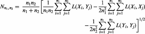(3)

Here, we consider only , the Euclidian distance in R^p. In the original papers, several other kernel functions, L were suggested as well (Baringhaus and Franz, 2004; Klebanov et al., 2007). N-statistic is actually a metric on the space of all probability measures on R^p (Klebanov et al., 2007).

Rotation gene set tests (ROAST) (Wu et al., 2010) uses the framework of linear models and tests whether for all genes in a set a particular contrast of the coefficients is non-zero (Wu et al., 2010). It can account for correlations between genes and has the flexibility of using different alternative hypotheses, testing whether the direction of changes for a gene in a set is ‘up’, ‘down’ or ‘mixed’ (up or down) (Wu et al., 2010). For all comparisons implemented here, the ‘mixed’ hypothesis was selected.

2.1.3 Univariate test

Gene-level tests for GSA can be easily designed in three steps: (i) select a gene-level score based on a univariate test statistic (e.g. a value of t-test) (ii) transform a score (e.g. take an absolute value of t-test, or consider its P-value) and (iii) summarize gene-level scores into a gene set statistic (e.g. take an average of transformed scores) (Ackermann and Strimmer, 2009). For instance, as a summary gene set statistic, the median and mean of gene-level P-values from t-tests were employed. We observed that the mean of P-values had less power compared with the median (data not shown). In the following, only results for the median of P-values (mpv-test) are presented.

Shrinking the standard error of a test statistic (e.g. a t-test) in testing differential expression of individual genes improves the power of the test. Several shrinkage approaches at the level of individual genes were suggested, including the Significance Analysis of Microarray (SAM) test (Tusher et al., 2001), the regularized t-test (Baldi and Long, 2001) and the moderated t-test (Smyth, 2004). An extension of SAM test to gene set analysis (SAM-GS) was also suggested (Dinu et al., 2007) and has been demonstrated to outperform several conventional self-contained tests, including competetive GSEA approach (Dinu et al., 2007, 2009; Liu et al., 2007). Therefore, we included SAM-GS in our comparative power analysis.

2.1.4 Significance testing

To estimate the null distribution of a test statistic numerically to obtain P-values, for all test statistics, except ROAST, 1000 sample permutations were used. ROAST uses a random rotation of the data matrix, which has been shown to give meaningful results, even for small sample sizes (Wu et al., 2010).

2.2 Simulation setup

In real biological settings not all genes in a gene set are differentially expressed, and intergene correlations vary in strength (Tripathi and Emmert-Streib, 2012). We therefore designed simulations specifically to be able to control: (i) the percentage of genes, truly differentially expressed between two phenotypes, parameter γ and (ii) the strength of the correlations between genes, parameter r. These parameters seriously influence the power of the test and it is important to understand the magnitude of influence for different tests statistics.

We simulated two samples of equal size, N/2 (N = 40, N = 20, N = 10) from the p-dimensional normal distribution and representing two biological conditions with different outcomes. We considered two scenarios: when the number of genes in a gene set (pathway), p is relatively small (p = 20) and relatively large (p = 100). The γ parameter, indicating the proportion of genes in a pathway under alternative hypothesis, was set to γ{0.25, 0.5, 0.75, 1}. To control the strength of intergene correlations for a gene set, three correlation regimes: low, medium and high (0.1, 0.5, 0.9) were simulated. Two alternative hypotheses were formulated:

H_a1. The mean vector for the first biological condition was fixed as 0 and all components of the mean vector, for the second biological condition were set to change from 0 to 2 with a step size of 0.2, that is was varied from to . The diagonal elements of the covariance matrix, i.e. variances of individual genes, were set to 1.

H_a2. The mean vectors for both conditions were fixed at but the diagonal elements of the covariance matrix , i.e. variances of individual genes, were fixed in one condition and set to change from 1 to 5 with a step size of 0.5 in the other.

For alternatives H_a1 and H_a2, different settings result in 24 and 6 simulated datasets, respectively. For each value of the mean or the variance, we averaged over 1000 independent runs (gene sets).

3 RESULTS

3.1 Simulation study

3.1.1 Type I error rate

Table 1 presents estimates for the attained significance levels of the seven tests. As can be seen, ROAST and SAM-GS provide more conservative estimates of the Type I error rate for small and medium intergene correlations than the N-statistic. In turn, the N-statistic controls the Type I error rate slightly better than non-parametric generalizations of the WW and KS tests, while the median P-values test shows the best control (Table 1).

Table 1.

Type I error rates for seven different test statistics in dependence on various correlation coefficient and pathway sizes p; α = 0.05, N = 40

rij	p = 20	p = 60	p = 100
N-statistic
rij = 0.1	0.0521	0.0499	0.0527
rij = 0.5	0.0525	0.0513	0.0534
rij = 0.9	0.0465	0.0526	0.0490
ROAST
rij = 0.1	0.0495	0.0479	0.0496
rij = 0.5	0.0515	0.0481	0.0498
rij = 0.9	0.0480	0.0521	0.0452
SAM-GS
rij = 0.1	0.0486	0.0459	0.0488
rij = 0.5	0.0491	0.0480	0.0492
rij = 0.9	0.0513	0.0560	0.0513
WW
rij = 0.1	0.0701	0.0666	0.0675
rij = 0.5	0.0736	0.0691	0.0711
rij = 0.9	0.0695	0.0703	0.0696
KS
rij = 0.1	0.0675	0.0693	0.0694
rij = 0.5	0.0680	0.0678	0.0706
rij = 0.9	0.0675	0.0691	0.0669
RKS
rij = 0.1	0.0634	0.0718	0.0662
rij = 0.5	0.0683	0.0696	0.0686
rij = 0.9	0.0707	0.0695	0.0687
Median of P-values
rij = 0.1	0.0000	0.0000	0.0000
rij = 0.5	0.0018	0.0020	0.0017
rij = 0.9	0.0192	0.0211	0.0169

3.1.2 The power of tests to detect shift alternatives

Figure 1 presents the results of power estimates, when H_a1 is true, for seven tests with p = 20 genes in a pathway. The parameter γ (the percentage of genes, truly differentially expressed between two phenotypes, γ {0.25, 0.5, 0.75, 1}) is increasing from the top to the bottom for all three columns. The parameter r{0.1, 0.5, 0.9} (intergene correlations) is increasing from the left to the right for all four rows.

Fig. 1.

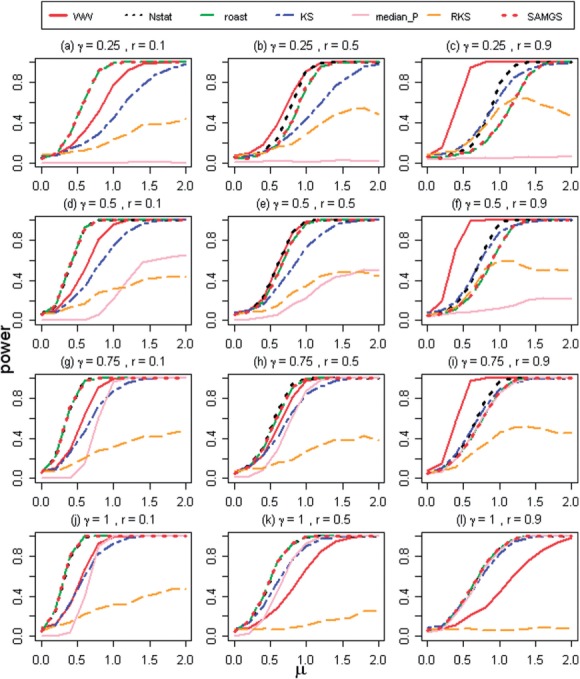
The power curves of seven tests when shift alternative hypothesis (H_a1) holds true and the number of genes in pathways p = 20 (N = 40)

First, consider the case, when all genes in a pathway are differentially expressed (γ = 1) and the intergene correlations are low (r = 0.1). In this case, the seven tests form three different groups (Fig. 1j). N-statistic, ROAST and SAM-GS have an identical power and form one group with a high power (HP) capable of detecting small changes; the median of P-values test (median of P-value test (mpv-test)), multivariate KS and WW tests form another group with a lower power (LP); the RKS test has almost no power (NP) to detect even large differences. This is actually what one would expect: the power of non-parametric tests is slightly lower than the power of parametric tests, the power of gene-level test without shrinking the standard error is lower than the power of the shrinkage (SAM-GS) and multivariate tests. The test sensitive for the scale alternative, expectedly, has almost no power to detect the shift alternative. This categorization remains unchanged (same tests belong to HP, LP, NP groups) even when we alter the number of differentially expressed genes, given the intergene correlations are still low (r = 0.1, first column of Fig. 1). Only the power of the mpv-test decreases to zero for γ = 0.25. Also, it should be noted that WW is becoming more powerful than KS when the γ parameter is decreasing.

Unexpected changes in the power curves are seen for higher correlations and γ {0.25, 0.5, 0.75} (middle column, bottom–up). Given r = 0.5, the content of the HP, LP, NP groups has been changed. Now the WW test joins the HP group, and only the KS test remains in the LP group. The power of the mpv-test decreases fast with γ. Further, the power of RKS remains low.

More dramatic changes in the power curves are seen when the intergene correlations become the highest (r = 0.9) and γ {0.25, 0.5, 0.75} (right-most column, Fig. 1). For these settings, the WW test outperforms all the others and populates along the HP group, whereas ROAST, SAM-GS, N-statistic and KS test form the LP group. As before, the power of the mpv-test decreases fast with γ. Again, the power of the N-statistic and the KS test is comparable and is becoming higher than the power of ROAST and SAM-GS when γ decreases.

The results for p = 100 (Supplementary Fig. S1) are similar to those for p = 20, but all the trends discussed above are more pronounced. In general, when p = 100, the power of all tests under different settings is higher and less dependent on γ. The power of the WW test is already higher than all the others when r = 0.5 and γ{0.25, 0.5, 0.75}. The power of the KS test is higher than the power of ROAST, SAM-GS and N-statistic when r = 0.9 and γ{0.25, 0.5, 0.75} (Supplementary Fig. S1, right-most column). The mpv-test has some power even when γ = 0.5.

To summarize, from the simulation results we can see that the power of all tests, except WW, decreases with the increase of intergene correlations. Unexpectedly, the power of WW test is higher than that of all the other tests when the intergene correlations are high: r{0.5, 0.9}, γ{0.25, 0.5, 0.75}. Notably, the power of the KS test is comparable with the N-statistic, ROAST and SAM-GS when simultaneously, γ decreases and the intergene correlations increase. RKS has almost no power in all conditions. The power of the mpv-test is similar (but lower) to ROAST, SAM-GS, KS and N-statistic when γ{1, 0.75}, but is very small when γ = 0.5 and decreases to zero when γ = 0.25. All these results are expected, except the result for the WW test. The question is: Why does WW outperform all other tests when γ{0.25, 0.5, 0.75} and the correlations are high?

To investigate the behavior of the WW test in these settings, we consider an example when p = 2 and there are two different phenotypes, X and Y from two bivariate normal distributions (Fig. 2). Consider the case when the intergene correlation is low (Fig. 2a) and either one (γ = 0.5), or two genes (γ = 1) in a pathway are differentially expressed (phenotypes Y_{γ = 0·5} and Y_{γ = 1}). Samples from two phenotypes (either X, Y_{γ = 0·5} or X, Y_{γ = 1}) are independent, scattered within two contours and the intersection areas between phenotypes X and Y_{γ = 0.5} and X and Y_{γ = 1} are of similar size. The number of disjoint subtrees obtained from the MST tree (R-statistic) is proportional to the number of samples from X and Y in a close proximity of each other. That means, when the correlation is low, the power of the WW test is similar for both cases, γ = 0.5 and γ = 1. When correlation is high (Fig. 2b), the samples are no longer independent and scattered in the same direction. If γ = 0.5, one gene is changing, and the distribution is shifted along one axis (45° with minor elliptical axis). If γ = 1, both genes are changing, and the distribution is shifted in the direction of the major elliptical axis. The difference in the shift directions results in a larger intersection area between X and Y_{γ = 1} when compared with X and Y_{γ = 0·5}, and as a consequence, a smaller power of the WW test for a high gamma and high correlations. This explanation can be generalized to cases with p > 2 and explains the high power exhibited by the WW test in Figure 1 when r = {0.5, 0.9} and γ = {0.25, 0.5, 0.75} compared with the low power when γ = 1.

Fig. 2.

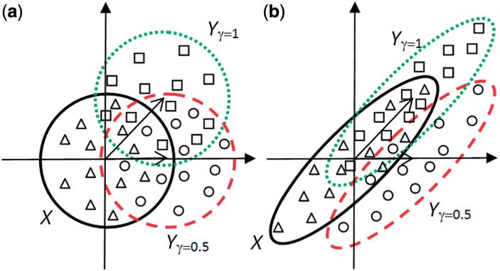
An example illustrating the effect of intergene correlation on the number of subtrees obtained from the MST when, (a) correlation is low and area(X ∩ Y_{γ = 0.5}) ≈ area(X ∩ Y_{γ = 1}), (b) correlation is high and area(X ∩ Y_{γ = 0·5}) < area(X ∩ Y_{γ = 1})

3.1.3 The power of tests to detect scale alternatives

Figure 3 presents the simulation results when H_a2 is true, for six tests with p = 20 genes in a pathway. The parameter r{0.1, 0.5, 0.9} (intergene correlations) is increasing from left to right. As expected, WW, ROAST, SAM-GS and KS have no power to detect changes in the scale, because they were not designed for this scenario. RKS has a high power to detect even small changes in the variance structure and outperforms the N-statistic for all values of the intergene correlations. The power of the N-statistic decreases significantly when the correlation increases to r = 0.9. Interestingly, in these settings, the WW test acquires some power that increases for large differences in scale (Fig. 3). The results for p = 100 (Supplementary Fig. S2) are similar to those for p = 20.

Fig. 3.

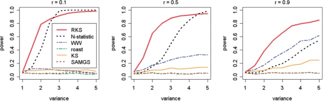
The power curves of six tests when scale alternative hypothesis (H_a2) holds true and the number of genes in a pathways p = 20 (N = 40)

For a sample size N = 20 the power of all tests was significantly smaller, however, the pattern of differences between the different tests remains the same (Supplementary Figs S3 and S4). However, with the smaller sample size (N = 10) all tests perform equally poor and comparative power analysis does not make sense anymore (Supplementary Figs S5 and S6). Because the result for ROAST and SAM-GS were almost identical in all settings, we did not include SAM-GS in the analysis of real data.

3.2 The analysis of solid tumors (kidney, lung and pancreas) expression arrays

Table 2 presents the overview of the datasets analyzed, selected from the comparative study of meta-analysis and integrated approaches in (Dawany and Tozeren, 2010). Data were normalized using the Robust Multi-array Average method and among multiple probes measuring the same target mRNA probes with maximum inter-quartile ranges (IQR) were selected. Half of the probes that exhibit the lowest variability (IQR) were filtered out, as recommended (e.g. by Bourgon et al., 2010; Hackstadt and Hess, 2009). At the end of these filtering steps, the final number of probes considered out of the total number for GSE7670, GSE15471 and GSE15641 were 6359 out of 22 283, 9899 out of 54 675 and 6359 out of 22 283.

Table 2.

Overview of the datasets used

Tissue	GEO ID	Samples	Affymetrix platform	Number of tested pathways
Lung	GSE7670	Normal 26 cancer 26	hgu133a	206
Pancreas	GSE15471	Normal 36 cancer 36	hgu133plus2	211
Kidney	GSE15641	Normal 23 cancer 32	hgu133a	209
Common				201

All three datasets (Table 2) have ‘normal’ and ‘cancer’ samples. To find pathways, differentially expressed between these two phenotypes, six aforementioned tests were applied, and the Kyoto Encyclopedia of Gene and Genome (KEGG) database (Kanehisa and Goto, 2000) was used as a source to define molecular pathways. Overall, three datasets had 201 KEGG pathways in common (Table 2). After controlling the false-discovery rate (FDR) at a level of 0.05 with the Benjamini and Hochberg (1995) procedure three tests, namely ROAST, N-statistic and WW (except for GSE7670) found all these pathways to be differentially expressed (Table 3). Although KS and the median P-values tests did not find all the pathways to be differentially expressed, the amount found was comparable (138–198 pathways). Finally, the RKS test has found 126, 169 and 131 pathways to be differentially expressed for the lung, pancreas and kidney cancer datasets, respectively. The result is similar to what one could expect from the simulation study. In most settings for the simulated data the N-statistic, ROAST and WW have had a better power than the KS, RKS and median P-values tests.

Table 3.

Number of differentially expressed KEGG pathways among the 201 common pathways in all three datasets

	Lung GSE7670	Pancreas GSE15471	Kidney GSE15641
ROAST	201	201	201
N	201	201	201
WW	200	201	201
KS	174	191	193
RKS	126	169	131
Median of P-values	138	198	194
RKS and not in KS	17	7	5
KS and not in RKS	65	29	67
Both KS and RKS	109	162	126

The rejection of the null hypothesis H₀ per se is important and informative. However, there are potentially many reasons for a rejection. Consider the most powerful test for the analysis of differentially expressed pathways, N-statistic which is designed to detect complex departures from the null hypothesis H₀, such as differences in marginal distributions, shift and scale alternatives and changes in the correlation structures. Therefore, if the null hypothesis is rejected by the N-statistic, we are not armed to dissect the specific alternative leading to rejection. Similarly, if ROAST or WW reject the null hypothesis, the true alternative hypothesis cannot be uniquely identified. The benefit of applying the new KS and RKS tests is that, while lacking the flexibility to test complex departures from H₀, they are designed to detect the simple alternatives: changes in the shift and scale. The knowledge about these specific alternatives can be important in interpreting the results. For this reason, we suggest using these two tests as complementary tools to clarify the cause for the rejection of the null hypothesis H₀ (see below).

From our analysis, we found 17, 7 and 5 pathways for GSE7670 (lung), GSE15471 (pancreas) and GSE15641 (kidney), respectively, only detected by RKS and not detected by KS, and there were 65, 29 and 67 pathways only detected by KS but not RKS (Table 3). RKS has the highest power to detect scale, whereas KS has the highest power to detect shift alternatives and in the pathways, detected exclusively by either one of them, exactly these two moments are changing. Figure 4 presents boxplots for the means and variances of genes, included in the pathways, detected by RKS only. As one can see, even the univariate differences in the mean variances between normal and cancer samples are very pronounced (Fig. 4a–c, right panels), more pronounced than differences in the univariate mean changes (Fig. 4a–c, left panels). Interestingly, for pathways detected by multivariate RKS and by both, RKS and KS tests, there is a good agreement between the multivariate tests and the univariate KS test of difference in the distributions of mean expression variances (Supplementary Table S1). However, there is no agreement between the univariate KS test of difference in the distributions of mean expressions and its multivariate counterpart (Supplementary Table S1). These observations underscore the high power of RKS to detect scale differences.

Fig. 4.

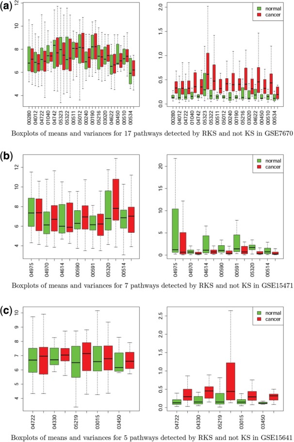
Boxplots of means and variances for pathways detected by RKS-only test for GSE7670, GSE15471 and GSE7670 series

Figure 5 presents boxplots and MST trees for three selected pathways (GSE15641, kidney cancer) detected by RKS only (Fig. 5a), KS only (Fig. 5b) and KS and RKS (Fig. 5c) tests. It is visually compelling that in all three cases the ‘amount’ of differences between the mean variances and the mean expressions between two phenotypes is in agreement with the test-specific alternatives. MST trees for the selected pathways (Fig. 5) show major differences. For the mRNA surveillance pathway (Fig. 5a), samples of one phenotype constitute the backbone of the MST, while samples of the other phenotype form the branches. Since the center node is naturally at the center of the backbone, there are significant differences in ranks assigned to two phenotypes. In contrast, for pathways detected by KS (Fig. 5b) and KS and RKS (Fig. 5c) on the corresponding MST trees samples of each phenotype are grouped together.

Fig. 5.

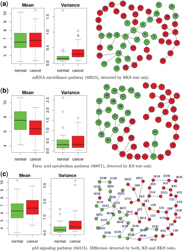
Selected pathways and their MST trees detected by (a) RKS, (b) KS and (c) RKS and KS tests in kidney cancer (GSE15641). Node ranks are given according to (a) RKS, (b) KS and (c) KS/RKS tests

Another important result is that pathways, detected exclusively by RKS (Supplementary Table S2) were tumor-specific, that means among them only one (‘Neurothrophin signaling pathway’, 04722) was simultaneously detected in two datasets (GSE7670, lung and GSE15641, kidney cancer data). Pathways, detected by the KS test only, were less specific: there were 8 and 21 common pathways, between GSE7670 (lung) and GSE15471 (pancreas), GSE15641 (kidney), respectively, and 9 common pathways between GSE15471 and GSE15641 (Supplementary Table S2). For all three datasets there was one pathway, ‘Circadian rhythm—mammal’ detected by KS as having differences in mean vectors between normal and cancer samples. Because the N-statistic detected all 201 pathways as being differentially expressed, not surprisingly, there were 53 pathways, detected simultaneously by RKS and KS in all three datasets (Supplementary Table S3). It may indicate that the rest of the pathways (that is pathways detected exclusively by the N-statistic, as well as ROAST and WW tests, and not by RKS and KS, or RKS only, or KS only) have a more complex departure from the null hypothesis H₀, than the scale and shift alternatives.

The analysis of the real data demonstrates that the N-statistic, ROAST and WW are robust and consistently detect any kind of departure from an alternative on a set of solid tumors. In turn, pathways, discovered exclusively by RKS or KS (to a smaller extent) highlight changes pertinent to a specific tumor.

4. DISCUSSION

Interpretation of the results of any large-scale genomic experiment is a challenge. Testing the differential expression of gene sets (GSA) is routinely used for gene expression data analysis (Ackermann and Strimmer, 2009; Emmert-Streib and Glazko, 2011; Hung et al., 2012) in particular, to gain more insights into specific pathways, underlying phenotypic changes. There are many self-contained GSA approaches available (Ackermann and Strimmer, 2009; Emmert-Streib and Glazko, 2011) but all of them have a potential weakness: the analysis result is difficult to interpret. For example, N-statistic, the most powerful multivariate test, has a complex alternative hypothesis: difference of two multivariate distributions (Klebanov et al., 2007). Similarly, tests employing aggregated score of gene-level test statistics do not have a well-specified alternative (Ackermann and Strimmer, 2009). Here, we demonstrate that the application of multivariate generalizations of the WW and KS (including RKS) non-parametric two-sample tests, that were developed by Friedman and Rafsky (1979), makes GSA approaches more comprehensive and helps to interpret the results better.

Our simulation study suggests that WW, KS and RKS all have specific characteristics important in the analysis of real biological data. Contrary to the conventional GSA multivariate tests (such as N-statistic and ROAST), the power of the WW test increases with the increase of the intergene correlations. This is an unexpected property suitable for the analysis of highly correlated expression data. In turn, the KS and RKS tests also have important differences from conventional tests: KS is exclusively sensitive to shift and RKS is mostly sensitive to scale alternatives, respectively. The analysis of real expression data confirms the major trends in the tests’ power, observed in simulations. Indeed, for all three expression datasets considered the WW test is as powerful as conventional approaches. In turn, RKS and KS tests can detect different alternatives.

From our analysis, we suggest the following approach for a GSA: first, use the most powerful multivariate test (e.g. N-statistic or WW test) for detecting all pathways for which the null hypothesis H₀ is rejected. Then, for a subset of these pathways the cause for their detection can be found by testing for a shift and scale alternatives, using KS or RKS. The pathways, selected under different alternatives potentially will help in interpreting the reasons of underlying phenotypic changes. The intersection of genes in these pathways can constitute a phenotype-specific gene signature, different for different alternatives and important in the follow-up studies.

There are many opportunities to improve the tests’ sensitivity and scope, provided by MST structure employed in non-parametric multivariate generalization of two-sample tests. For instance, a MST tree can be constructed using any dissimilarity measure and for any types of data (on an ordinal or ratio scale). That means the multivariate generalization of KS and WW are readily applicable for the analysis of RNA-Seq data, represented by read counts. Further, for such data a different dissimilarity measure than that used in our study (Euclidean distance) may lead to differences in the observed power. Another interesting opportunity provided by a MST structure is in defining a pertinent procedure for a subtrees ranking that can be sensitive to various alternatives. We conclude that the use of the multivariate non-parametric generalization of two-sample tests and the exploration of their potential improvement can increase our ability to interpret the results of large-scale expression experiments and dissect relevant biological processes leading to phenotypic changes between two conditions.

References

- Ackermann M, Strimmer K. A general modular framework for gene set enrichment analysis. BMC Bioinformatics. 2009;10:47. doi: 10.1186/1471-2105-10-47. [DOI] [PMC free article] [PubMed] [Google Scholar]
- Allison DB, et al. Microarray data analysis: from disarray to consolidation and consensus. Nat. Rev. Genet. 2006;7:55–65. doi: 10.1038/nrg1749. [DOI] [PubMed] [Google Scholar]
- Baldi P, Long AD. A Bayesian framework for the analysis of microarray expression data: regularized t -test and statistical inferences of gene changes. Bioinformatics. 2001;17:509–519. doi: 10.1093/bioinformatics/17.6.509. [DOI] [PubMed] [Google Scholar]
- Baringhaus L, Franz C. On a new multivariate two-sample test. J. Multivariate Anal. 2004;88:190–206. [Google Scholar]
- Benjamini Y, Hochberg Y. Controlling the false discovery rate: A practical and powerful approach to multiple testing. J. Roy. Statist. Soc. B. 1995;57:289–300. [Google Scholar]
- Bourgon R, et al. Independent filtering increases detection power for high-throughput experiments. Proc. Natl Acad. Sci. USA. 2010;107:9546–9551. doi: 10.1073/pnas.0914005107. [DOI] [PMC free article] [PubMed] [Google Scholar]
- Dawany NB, Tozeren A. Asymmetric microarray data produces gene lists highly predictive of research literature on multiple cancer types. BMC Bioinformatics. 2010;11:483. doi: 10.1186/1471-2105-11-483. [DOI] [PMC free article] [PubMed] [Google Scholar]
- Dinu I, et al. Improving gene set analysis of microarray data by SAM-GS. BMC Bioinformatics. 2007;8:242. doi: 10.1186/1471-2105-8-242. [DOI] [PMC free article] [PubMed] [Google Scholar]
- Dinu I, et al. Gene-set analysis and reduction. Brief. Bioinform. 2009;10:24–34. doi: 10.1093/bib/bbn042. [DOI] [PMC free article] [PubMed] [Google Scholar]
- Emmert-Streib F. The chronic fatigue syndrome: a comparative pathway analysis. J. Comput. Biol. 2007;14:961–972. doi: 10.1089/cmb.2007.0041. [DOI] [PubMed] [Google Scholar]
- Emmert-Streib F, Glazko GV. Pathway analysis of expression data: deciphering functional building blocks of complex diseases. PLoS Comput. Biol. 2011;7:e1002053. doi: 10.1371/journal.pcbi.1002053. [DOI] [PMC free article] [PubMed] [Google Scholar]
- Friedman J, Rafsky L. Multivariate generalization of the Wald-Wolfowitz and Smirnov two-sample tests. Ann. Stat. 1979;7:697–717. [Google Scholar]
- Gatti DM, et al. Heading down the wrong pathway: on the influence of correlation within gene sets. BMC Genomics. 2010;11:574. doi: 10.1186/1471-2164-11-574. [DOI] [PMC free article] [PubMed] [Google Scholar]
- Glazko GV, Emmert-Streib F. Unite and conquer: univariate and multivariate approaches for finding differentially expressed gene sets. Bioinformatics. 2009;25:2348–2354. doi: 10.1093/bioinformatics/btp406. [DOI] [PMC free article] [PubMed] [Google Scholar]
- Goeman JJ, Buhlmann P. Analyzing gene expression data in terms of gene sets: methodological issues. Bioinformatics. 2007;23:980–987. doi: 10.1093/bioinformatics/btm051. [DOI] [PubMed] [Google Scholar]
- Hackstadt AJ, Hess AM. Filtering for increased power for microarray data analysis. BMC Bioinformatics. 2009;10:11. doi: 10.1186/1471-2105-10-11. [DOI] [PMC free article] [PubMed] [Google Scholar]
- Huang da W, et al. Bioinformatics enrichment tools: paths toward the comprehensive functional analysis of large gene lists. Nucleic Acids Res. 2009;37:1–13. doi: 10.1093/nar/gkn923. [DOI] [PMC free article] [PubMed] [Google Scholar]
- Hung JH, et al. Gene set enrichment analysis: performance evaluation and usage guidelines. Brief. Bioinform. 2012;13:281–291. doi: 10.1093/bib/bbr049. [DOI] [PMC free article] [PubMed] [Google Scholar]
- Jiang Z, Gentleman R. Extensions to gene set enrichment. Bioinformatics. 2007;23:306–313. doi: 10.1093/bioinformatics/btl599. [DOI] [PubMed] [Google Scholar]
- Kanehisa M, Goto S. KEGG: kyoto encyclopedia of genes and genomes. Nucleic Acids Res. 2000;28:27–30. doi: 10.1093/nar/28.1.27. [DOI] [PMC free article] [PubMed] [Google Scholar]
- Klebanov L, et al. A multivariate extension of the gene set enrichment analysis. J. Bioinform. Comput. Biol. 2007;5:1139–1153. doi: 10.1142/s0219720007003041. [DOI] [PubMed] [Google Scholar]
- Kong SW, et al. A multivariate approach for integrating genome-wide expression data and biological knowledge. Bioinformatics. 2006;22:2373–2380. doi: 10.1093/bioinformatics/btl401. [DOI] [PMC free article] [PubMed] [Google Scholar]
- Liu Q, et al. Comparative evaluation of gene-set analysis methods. BMC Bioinformatics. 2007;8:431. doi: 10.1186/1471-2105-8-431. [DOI] [PMC free article] [PubMed] [Google Scholar]
- Lu Y, et al. Hotelling's T2 multivariate profiling for detecting differential expression in microarrays. Bioinformatics. 2005;21:3105–3113. doi: 10.1093/bioinformatics/bti496. [DOI] [PubMed] [Google Scholar]
- Montaner D, et al. Gene set internal coherence in the context of functional profiling. BMC Genomics. 2009;10:197. doi: 10.1186/1471-2164-10-197. [DOI] [PMC free article] [PubMed] [Google Scholar]
- Mootha VK, et al. PGC-1alpha-responsive genes involved in oxidative phosphorylation are coordinately downregulated in human diabetes. Nat. Genet. 2003;34:267–273. doi: 10.1038/ng1180. [DOI] [PubMed] [Google Scholar]
- Smyth GK. Linear models and empirical bayes methods for assessing differential expression in microarray experiments. Stat. Appl. Genet. Mol. Biol. 2004;3:Article3. doi: 10.2202/1544-6115.1027. [DOI] [PubMed] [Google Scholar]
- Tian L, et al. Discovering statistically significant pathways in expression profiling studies. Proc. Natl Acad. Sci. USA. 2005;102:13544–13549. doi: 10.1073/pnas.0506577102. [DOI] [PMC free article] [PubMed] [Google Scholar]
- Tripathi S, Emmert-Streib F. Assessment method for a power analysis to identify differentially expressed pathways. PLoS One. 2012;7:e37510. doi: 10.1371/journal.pone.0037510. [DOI] [PMC free article] [PubMed] [Google Scholar]
- Tusher VG, et al. Significance analysis of microarrays applied to the ionizing radiation response. Proc. Natl Acad. Sci. USA. 2001;98:5116–5121. doi: 10.1073/pnas.091062498. [DOI] [PMC free article] [PubMed] [Google Scholar]
- Wang X, et al. Linear combination test for hierarchical gene set analysis. Stat. Appl. Genet. Mol. Biol. 2011;10:Article 13. doi: 10.2202/1544-6115.1641. [DOI] [PubMed] [Google Scholar]
- Wu D, et al. ROAST: rotation gene set tests for complex microarray experiments. Bioinformatics. 2010;26:2176–2182. doi: 10.1093/bioinformatics/btq401. [DOI] [PMC free article] [PubMed] [Google Scholar]
- Xiong H. Non-linear tests for identifying differentially expressed genes or genetic networks. Bioinformatics. 2006;22:919–923. doi: 10.1093/bioinformatics/btl034. [DOI] [PubMed] [Google Scholar]
Associated Data
This section collects any data citations, data availability statements, or supplementary materials included in this article.