Site identification in high-throughput RNA–protein interaction data

Abstract

Motivation: Post-transcriptional and co-transcriptional regulation is a crucial link between genotype and phenotype. The central players are the RNA-binding proteins, and experimental technologies [such as cross-linking with immunoprecipitation- (CLIP-) and RIP-seq] for probing their activities have advanced rapidly over the course of the past decade. Statistically robust, flexible computational methods for binding site identification from high-throughput immunoprecipitation assays are largely lacking however.

Results: We introduce a method for site identification which provides four key advantages over previous methods: (i) it can be applied on all variations of CLIP and RIP-seq technologies, (ii) it accurately models the underlying read-count distributions, (iii) it allows external covariates, such as transcript abundance (which we demonstrate is highly correlated with read count) to inform the site identification process and (iv) it allows for direct comparison of site usage across cell types or conditions.

Availability and implementation: We have implemented our method in a software tool called Piranha. Source code and binaries, licensed under the GNU General Public License (version 3) are freely available for download from http://smithlab.usc.edu.

Contact: andrewds@usc.edu

Supplementary information: Supplementary data available at Bioinformatics online.

1 INTRODUCTION

Originally thought simply to be a vehicle for the transport of genetic information, RNA has come to be seen as a crucial nexus for eukaryotic diversity and control of expression (Licatalosi and Darnell, 2010; Sharp, 2009). The mechanisms which govern this are diverse and include splicing, localization, polyadenylation and the control of both transcript stability and abundance. RNA-binding proteins (RBPs), which associate with RNA through specialized protein domains called RNA-binding domains, drive these processes. The activities of these proteins can be complex and involve not only other proteins but also other RNA species (Kedde et al., 2010; Kloosterman and Plasterk, 2006; le Sage et al., 2007; Siomi and Siomi, 2009). The functions of some RBPs are so essential that perturbation of their activity can lead to remarkable phenotypic changes (Chénard and Richard, 2008; Lukong et al., 2008; Lunde et al., 2007; Wang et al., 2010a).

Understanding the functions and mechanisms of the many RBPs is one of the key challenges currently facing cellular biology. Despite tremendous recent progress, there are still many unanswered questions (König et al., 2012; Wang et al., 2010a). Perhaps the most direct approach to profiling these interactions is the immunoprecipitation of the RBP of interest through a process similar in principle to chromatin immunoprecipitation (ChIP). Modern high-throughput immunoprecipitation assays for protein–RNA interaction can trace their lineage back to RIP-chip, an array-based assay (Tenenbaum et al., 2000). Cross-linking with immunoprecipitation (CLIP) extended upon the success of RIP-Chip by introducing ultraviolet cross-linking of the protein to the RNA and more stringent washing to increase specificity, though potentially at the cost of reduced sensitivity (Ule et al., 2005). More recently, CLIP has been coupled with high-throughput sequencing (HITS-CLIP) to enable a much greater range and depth of coverage (Licatalosi and Darnell, 2010). Further improvements to allow single-nucleotide resolution have been achieved by iCLIP (Konig et al., 2010) and photoactivatable-ribonucleoside-enhance CLIP (PAR-CLIP) variants (Hafner et al., 2010).

There are substantial challenges to be overcome in terms of the effective analysis of CLIP-seq data however. In this article, our focus is on-site identification (or, peak-calling), which is the crucial step that follows mapping of reads to a reference and deals with identifying those genomic locations that are true protein interaction sites. For simplicity, we refer to this step as site identification regardless of the resolution. That is to say, the process may be as coarse-grained as calling target transcripts or as fine-grained as identifying sites at a single-nucleotide level.

We begin by outlining three key challenges in RBP site identification. The first is intrinsic to the peak-calling process: many sites to which reads map only receive a very small number of reads and are likely noise. The levels of noise may be far from negligible and have multiple causes. The sequenced sample may contain RNA that has not been cross-linked to a protein or alternatively that was cross-linked to some different protein, but pulled down through antibody cross-reactivity. In addition, reads can map to non-target transcripts due to sequencing errors or mapping problems. Effective use of the data requires separating these noise sites or false positives, from functional sites. Most studies, explicitly or implicitly, assume read counts at individual sites, follow a particular distribution and use this distribution to determine the probability of seeing a given number of reads at a site by chance. However, there has been no large-scale analysis of CLIP- and RIP-seq data to determine the most appropriate choice of distribution to model these counts.

The second challenge is somewhat more esoteric. The proportion of total reads falling in a given transcript does not give the probability of that transcript being a target, but rather informs the probability that a bound RNA is of that transcript. No knowledge of the number of unbound copies is available and hence the RBPs preference for that transcript is not directly discernible. This is true at higher resolutions also. Reads accumulate in transcripts in proportion not only to the RBPs preference for that transcript but also the transcript abundance. This is in contrast to ChIP, where there is (in general) no variation in multiplicity between different parts of the genome.

The final challenge we consider is that of incorporating external information into the peak-calling process. There are a number of types of external information, but here we consider what is essentially control data. We give details of other external information in Supplementary Material.

Previous studies involving CLIP-seq data have applied a range of different approaches to site identification. Because of the high fidelity of the CLIP assay, it is possible to side step the problem and retain all sites (Licatalosi et al., 2008). This does not allow for the filtering of noise interactions. Another simple approach is to take the top n sites under some scoring, such as normalized read count. This requires selecting a threshold, usually arbitrarily and clearly prevents comparing the number of sites between RBPs or conditions (Hafner et al., 2010; Kishore et al., 2011). More sophisticated methods employ a simulation of the CLIP-seq experiment assuming no site-specific preference and use this to arrive at a false discovery rate for any given peak height (Chi et al., 2009; Konig et al., 2010; Leung et al., 2011; Yeo et al., 2009). Although this allows for consideration of transcript abundance, there is no mechanism to explicitly adjust for other sequencing biases and the approach is not applicable to situations, where a second condition or control is available (e.g. RIP-seq).

Finally, some site identification methods intrinsically consider information specific to a particular immunoprecipitation assay (Corcoran et al., 2011; Hafner et al., 2010; Lebedeva et al., 2011; Zhang and Darnell, 2011). Although these have been highly successful, they cannot be applied in the more general setting.

Several databases of CLIP-seq data also exist, for example CLIPZ, StarBase and doRiNA (Anders et al., 2012; Khorshid et al., 2011; Yang et al., 2011). The latter two focuses on microRNA (miRNA)–RBP interactions. CLIPZ and StarBase group reads into clusters but do not perform any further site identification. In contrast, doRiNA uses a site identification strategy for PAR-CLIP that relies upon T to C conversions at the cross-link site, but is unable to automatically score or rank sites from RIP-seq or other CLIP-seq variants.

We present a method for site identification that is applicable across the three commonly used CLIP-seq variants and in addition can be applied to RIP-seq data (for which, to our knowledge, no peak-calling tools currently exist). Our method addresses each of the three challenges outlined earlier: effectively modeling the underlying distribution, utilizing transcript abundance information and flexibly allowing the incorporation of external data. Further, we demonstrate how such a tool can be applied to answer more advanced biological questions regarding RBP binding sites that vary in usage between different cell types, conditions or stages of development.

2 METHODS

2.1 Data

We compiled all CLIP-seq (HITS, iCLIP and PAR-CLIP) datasets that were publicly available at the time of writing (see Table 1). In addition, we analyzed a previously unpublished HITS-CLIP dataset for Ago2/miR-124 and a RIP-seq dataset for hTra2, which we briefly describe.

Table 1.

We assembled a large collection of CLIP- and RIP-Seq datasets representing 22 distinct RBPs, 6 cell types and 4 technologies (iCLIP, HITS-CLIP, PAR-CLIP and RIP-Seq)

RBP	Technology	Cell	Citation
Ago	HITS-CLIP	HeLa	Chi et al. (2009)
Ago{1 … 4}, IGF2BP{1 … 3}, PUM2, QKI, TNRC6{A … C}	PAR-CLIP	HEK293	Hafner et al. (2010)
HnRNPH	HITS-CLIP	HEK293	Katz et al. (2010)
Ago2, HuR	HITS-CLIP, PAR-CLIP	HEK293	Kishore et al. (2011)
Fox2	HITS-CLIP	hESC	Yeo et al. (2009)
hnRNPC	iCLIP	HeLa	Konig et al. (2010)
HuR	PAR-CLIP	HeLa	Lebedeva et al. (2011)
HuR	PAR-CLIP	HEK293	Mukherjee et al. (2011)
HuR	iCLIP	HeLa	Uren et al. (2011)
Ago2	HITS-CLIP	mESC	Leung et al. (2011)
TIA1, TIAL1	iCLIP	HeLa	Wang et al. (2010b)
PTB	HITS-CLIP	HeLa	Xue et al. (2009)
TDP43	HITS-CLIP	Mouse brain	Polymenidou et al. (2011)
TDP43	iCLIP	SH-SY5Y	Tollervey et al. (2011)
Nova	HITS-CLIP	Brain	Zhang et al. (2010)
Ago2	HITS-CLIP	HEK293	This publication
hTra2	RIP-seq	HeLa	This publication

For the identification of miR-124-guided Ago2 binding sites by CLIP, 5 cm × 15 cm plates of 293S cells at 70% confluency per condition/replicate were used. Cells were transfected for 24 h with 100 nM mir-124 siRNA (5′-UAAGGCACGCGGUGAAUGCCA-3′ and 5′-GCAUUCACCGCGUGCCUUACA-3′ duplex) or control gl3.1 siRNA (5′-CUUACGCUGAGUACUUCGAUU-3′ and 5′-UCGAAGUACUCAGCGUAAGUU-3′ duplex) using Mirus Trans-IT TKO. The CLIP procedure was carried out by a modified protocol of Chi et al. (2009) as described in Supplementary Material.

The RIP protocol used for hTra2 is as follows: 400 μl of Protein A sepharose (50% slurry) was washed five times with NT2 buffer (50 mM Tris–HCl pH 7.4, 1 M Tris–HCl, 150 mM NaCl, 1 mM MgCl₂, 0.05% NP40) and resuspended in 1 ml of NT2 plus 5% BSA and 10 μg of rabbit anti-hTRA2B (Abcam) or normal rabbit IgG. Beads plus antibodies were incubated overnight at 4°C with rotation and washed five times with cold NT2 buffer. Lysates were prepared from semi-confluent HeLa cells in polysomal lysis buffer (10 mM HEPES pH 7.0, 100 mM KCl, 5 mM MgCl₂, 0.5% NP40, 2 mM dithiothreitol) containing proteinase and RNA inhibitors. After centrifugation for 10 min, supernatant was adjusted to 2 mg/ml and 6 ml of lysate were combined with the bead/antibody and rotated at room temperature for 3–5 h. Beads were washed five times with cold NT2. After last wash samples were digested with RNase III; 4 μl of RNaseIII (Ambion) were combined with 600 μl of 1× buffer, added to samples and incubated for 30 min at 37°C with agitation. Beads were recovered by centrifugation and washed three times with NT2 buffer. Proteins were extracted with 25 μl (20 mg/ml) proteinase K in 600 μl of 1× buffer at 50°C for 30 min. Samples were vortexed for 1 min and beads pelleted by centrifugation. The supernantant was extracted with 700 μl of acid phenol–chloroform and precipitated with sodium acetate and isopropanol. RNA was recovered by centrifugation, washed and resuspended in 13 μl of RNase free water. Quantity and quality were checked with Nanodrop and Bioanalyzer. Fifty nanograms of RNA were amplified using Nugen Ovation RNA-seq System I and libraries prepared with the Nugen Encore NGS Library System I per manufacturer’s protocol.

To adjust for transcript abundance, we also make use of RNA-seq data for HeLa cells (Uren et al., 2011) and HEK293 cells. All previously unpublished sequence data have been deposited into the sequence read archive (SRA), accession numbers: SRA056343, SRA056308, SRA056344.

2.2 Pre-processing

For each dataset, we trimmed adapters and mapped to an appropriate reference genome (full genome—hg19 or mm9) and junction database using rmap (Smith et al., 2009). Transcripts were defined per the University of California Santa Cruz (UCSC) genome browser known-genes track. We allowed up to three mismatches when mapping and retained only reads that unambiguously mapped to a single location. Junction reads were split and assigned to both side of the junction. Full details of the mapping results are given in Supplementary Material. Our method does not depend on any particular mapping or pre-processing strategy. Research is ongoing with respect to the most effective methods for mapping RNA reads and will be further spurred on as immunoprecipitation-based assays are paired with emerging sequencing platforms promising longer read lengths. Coupled with an effective choice of mapping and pre-processing techniques, our site identification method will remain relevant.

2.3 Peak finding

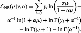
The input for site identification is a set of reads mapped to the reference genome. All reads are binned based on the nucleotide at which they begin. A bin represents a genomic interval and can be single nucleotide in width. Appropriate choice of bin size is dependent on depth of coverage and technology used (see Section 3.3). Let y_i be the count of the number of reads which start in the ith bin. Each bin optionally has an associated vector of covariates, which we denote . A covariate is a measure of some property that is expected to vary in parallel with the immunoprecipitation read counts, but need not be count data. An example is mappability of the bin, a measure of how many locations within the bin start sequences of length equal to the read length, which are not duplicated elsewhere in the genome and hence can be non-ambiguously mapped to. Bins with low mappability are expected to correlate with lower read count. We model the read counts within bins using a zero-truncated negative binomial distribution (see Section 3.2 for justification). Read counts from high-throughput immunoprecipitation experiments are Poisson over-dispersed. The negative binomial is an appropriate choice of distribution for dealing with Poisson over-dispersion, but does not correctly handle the adjusted weight for zero observations. One option is to use the zero-inflated negative binomial, as was adopted by the zero-inflated negative binomial algorithm (ZINBA) for peak calling in ChIP-seq data (Rashid et al., 2011). However, the zero-inflated negative binomial assumes a mixture, where a certain number of zeros are drawn from the negative binomial component (and the remainder from the zero-inflated component); this does not genuinely reflect the true underlying distribution, which does not produce zeros. Moreover, the additional complexity makes model fitting more difficult and time consuming. Instead, we retain only those bins with one or more reads mapping. We discuss this further in Supplementary Material. The zero-truncated negative binomial (ZTNB) has the following log-likelihood function:

(1)

where μ is the (un-truncated) mean, α is the dispersion parameter and is the log-likelihood of the non-adjusted negative binomial, that is

(2)

We fit the model by finding the maximum likelihood estimates for μ and α. We assume that the majority of sites with reads are low-occupancy or noise sites (see Section 3.2 for details and justification) and so the fit model represents a background. At an abstract level, our method is modeling the read-count distribution of the dataset, which is an acceptable proxy for the background noise distribution. We then look for locations with read counts that are unexpectedly large based on this theoretical distribution. To do this, after model fitting, each bin is assigned a P-value by subtracting from 1 the sum of densities for all values less than the read count associated with that bin. Significant bins can then be selected by a P-value threshold; the smaller the P-value, the more unlikely the read count in the bin is given the fit distribution.

When additional external data (covariates) are available, we use a zero-truncated negative binomial regression (ZTNBR) model (Cameron and Trivedi, 2008; Hilbe, 2011). Briefly, this requires replacing the scalar parameter μ with a vector , where each 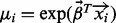and is the vector of regression coefficients. The model is fit using a Newton–Raphson algorithm for the estimation of the regression parameters and a dispersion dampening algorithm for estimating α (Hilbe, 1993, 2011). Each bin is assigned a P-value in the same way as previously described. A short illustration of applying the regression model to calculate P-values is given in Table 2. Notice how large read counts do not necessarily lead to significant P-values. A full description of the model, its derivation and fitting is provided in Supplementary Material.

Table 2.

Example of calculating P-values for bins using the ZTNBR with two covariates: mappability (X₁, in arbitrary units) and transcript abundance (X₂, in reads mapped from RNA-seq control), assuming the model has already been fit with β = 0.17, 0.02 and α = 2

Y				P-value
1	4	10	exp(0.17 × 4 + 0.02 × 10) = 2.41	1 − Pr(yi = j |μ = 2.41, α = 2) = 0.71
3	2	37	exp(0.17 × 2 + 0.02 × 37) = 2.94	1 − Pr(yi = j |μ = 2.94, α = 2) = 0.45
250	5	30	exp(0.17 × 5 + 0.02 × 30) = 4.26	1 − Pr(yi = j |μ = 4.26, α = 2) < 8.63 × 10−14 ***
5	4	17	exp(0.17 × 4 + 0.02 × 17) = 2.77	1 − Pr(yi = j |μ = 2.77, α = 2) = 0.27
7	7	13	exp(0.17 × 6 + 0.02 × 13) = 3.60	1 − Pr(yi = j |μ = 3.60, α = 2) = 0.24
300	10	180	exp(0.17 × 10 + 0.02 × 180) = 200.34	1 − Pr(yi = j |μ = 200.34, α = 2) = 0.23

2.4 Implementation and post-processing

Our method has been implemented in a software tool called Piranha. When no covariates are provided, it will fit a ZTNB model. If covariates are provided, it will fit a ZTNBR model. Input may be either raw reads in browser extensible data (BED) or binary sequence alignment/map (BAM) format, or pre-binned read counts in BED format. Covariates are provided in BED format. Output is in an extended BED format, where an additional column gives the P-value. The implementation and instructions for its use are given at http://smithlab.usc.edu

For the analysis in this article, we adjust output P-values to correct for multiple hypothesis testing using the method of Benjamini and Hochberg (1995).

3 RESULTS AND DISCUSSION

3.1 Alternative methods

Two recent approaches have been proposed specifically for addressing the problem of site identification in CLIP-seq data (Corcoran et al., 2011; Zhang and Darnell, 2011). Zhang’s method works on HITS-CLIP data and employs cross-linking-induced mutation sites (CIMS, primarily deletions) to refine site location, while PARalyzer is designed for PAR-CLIP data and relies on T to C conversions at the cross-link site. In contrast, the method we propose works on all CLIP-seq variants (iCLIP, PAR-CLIP, HITS-CLIP), as well as RIP-seq, while still being able to consider the positional deletion and mutation information used in these two methods as covariates. Further, our method allows the consideration of additional covariates (such as transcript abundance, which we demonstrate impacts read counts considerably). Moreover, Zhang et al. (2010) found that deletion events occur only in ∼8–20% of mRNA tags, meaning a substantial proportion of reads would not be informative, while our method can take advantage of all the mapped reads in each study. PARalyzer is publicly available and we compare its performance to our method (details of usage are in Supplementary Material); The CIMS-based method has no public implementation at the time of writing.

3.2 Read counts follow a zero-truncated negative binomial distribution

For each dataset, we estimated the parameters of a zero-truncated Poisson, negative binomial and zero-truncated negative binomial distribution for the counts when binned at single-nucleotide resolution. Figure 1A and B shows visually the improved fit provided by the ZTNB when compared to the NB; both panels show the average density of the real data in red and all of the fit densities for the NB and ZTNB in blue and green, respectively. To validate the improvement seen visually in Figure 1A and B we conducted a set of Pearson’s χ² tests. For 90.8% (109 of 120) of the datasets, the Pearson’s χ² test showed that the zero-truncated negative binomial provides a superior fit to a Poisson, zero-truncated Poisson or regular negative binomial distributions (see Fig. 1C for an example and Supplementary Table S2 for the complete set of results from the χ² tests). The majority of sites with reads mapping are low-occupancy or noise sites (Fig. 1D); in most of the datasets analyzed, >80% of locations with reads mapping saw <5 reads. Theoretically, read counts at sites are a mixture, with some drawn from a foreground distribution and some from a background noise distribution. In practice, though the mixing parameter is so heavily weighted toward the background that parameter estimates for the whole data closely approximate the background component. This is one reason that we eschew fitting a mixture and instead prefer the simpler single distribution.

Fig. 1.

CLIP read counts are fit well by zero-truncated negative binomial. (A) The average read count density for all datasets is shown in red (error bars are 95% confidence interval). The fitted densities for a negative binomial on all of the datasets is shown in blue (note that all densities are shown, rather than an average for each read count). Only read counts <20 are shown. (B) As with (A), but replacing the fit densities from the negative binomial with those of a zero-truncated negative binomial distribution. (C) Histogram of read counts from an iCLIP experiment for TIA1 (Wang et al., 2010b) showing fit zero-truncated Poisson, negative binomial and zero-truncated negative binomial distributions. (D) Histogram showing the count of datasets for which 80% of the locations receiving reads have no more reads than the given count; the majority of datasets have >80% of their locations with <5 reads. Four outliers are not shown, with read counts of 79, 93, 88 and 228

3.3 Read count is correlated with transcript abundance

The most common approach for site identification is a threshold. Applying a single threshold across the whole transcriptome is problematic since it does not consider transcript abundance. To quantify this, we compared RNA-seq data from HeLa and HEK293 to those IP experiments conducted in these cell lines. We observed a substantial positive correlation between RNA-seq read counts for a transcript and IP read counts (see Fig. 2A for the distribution of correlation coefficients and Fig. 2B for an example dataset), with an average correlation coefficient of 0.36 over the 85 datasets examined. We also compared 200 nt bins (see Fig. 2C) to ascertain the extent to which this relationship holds at a more fine-grained level. Here, we observed a lesser, but still substantial degree of correlation, with an average correlation coefficient of 0.16.

Fig. 2.

CLIP- and RIP-seq read counts are correlated with transcript abundance. (A) Distribution of Spearman correlation coefficients for RNA-seq and immunoprecipitation read counts at transcript level over all examined datasets shows frequent strong correlation (B) Example hexbin plot showing transcript-level correlation between IP read count for HuR (selected at random from the set of highly correlated datasets; data from Mukherjee et al., 2011) and RNA-seq read count in HEK293 cells. Spearman correlation coefficient: 0.67 (C) As in (A), but with 200 nt-wide non-overlapping bins; correlation is reduced in smaller bins, but still present

To address the problem of varying transcript abundance, we incorporate an RNA-seq control into our peak calling by supplying it as a covariate for the ZTNB regression method of Piranha. For this analysis, we considered a bin size of 200 nt, as was used earlier. An appropriate choice of bin size is dependent on the technology used and sequencing depth. Here, we have opted to select a bin size that allows us to capture the correlation between IP and RNA-seq given the level of coverage we have and is generally appropriate across all of the technologies profiled.

The number of experimentally verified binding sites for any given RBP is currently too low to realistically be used as a gold standard for peak calling. Instead, we turn to motif enrichment as a measure of accuracy—a similar approach was taken by Zhang and Darnell (2011). To be agnostic of existing characterizations of an RBPs motif, we perform de novo motif discovery for each dataset and consider the top enriched motif to be the correct one. For motif discovery, we use the DME algorithm (Smith et al., 2005). Full details of the scoring method used are given in Supplementary Material. We observed an average 11.6% improvement in motif score on the examined datasets when using the ZTNBR with RNA-seq covariate over the regular ZTNB (P < 5.9 × 10⁻³, Wilcoxon test), demonstrating that inclusion of this additional data can improve site identification.

We compared the performance of our method to PARalyzer, the only other publicly available site identification tool for CLIP-seq data. On PAR-CLIP datasets (which it is designed for), PARalyzer scores are on an average 3% better than ZTNB; however, the difference is not statistically significant. On an average the ZTNBR with transcript abundance covariate scores 17.2% higher (P < 0.002, Wilcoxon test). Full details are given in Supplementary Material.

3.4 Incorporating general external information

3.4.1 Using non-specific antibody controls in RIP-seq data

RIP-seq is not as specific as CLIP-seq, but is a more sensitive assay. An additional immunoprecipitation experiment using a non-specific antibody acts as a control. The appropriate use of this control in a statistically sound and robust fashion is essential for site identification in RIP-seq data; to our knowledge, no tools currently exist for this task. Piranha is able to use the non-specific antibody control as a covariate when calling peaks.

We applied our method to a RIP-seq dataset for hTra2, a ubiquitously expressed member of the serine/argenine-rich protein family. hTra2 functions as a splicing regulator, with its aberrant activity implicated in several diseases (Cléry et al., 2011; Gabriel et al., 2009; Hirschfeld et al., 2009; Hofmann et al., 2000; Sumner, 2007; Tsuda et al., 2011). The canonical hTra2 binding site is the (GAA)₂ repeat (Tsuda et al., 2011).

We provide the non-specific antibody control as a covariate to our zero-truncated negative binomial regression method. After selection of those sites which are significant, we performed de novo motif detection. The top identified motif enriched around the sites we identified is a match for the previously known (GAA)₂ motif and shows preferential localization near significant RIP-seq sites (see Fig. 3A). To determine whether the use of the non-specific antibody improves performance, we also ran Piranha without this extra input. Although the motif found is the same, we observe an increased occurrence around sites identified when using the non-specific antibody control. This demonstrates that our peak-calling tool can successfully be applied not only to CLIP-seq but also RIP-seq data. Full details of the hTra2 analysis, including identified sites, are given in Supplementary Material.

Fig. 3.

(A) Top identified motif and motif occurrence histogram for hTra2 identified from RIP-seq data using ZTNBR with non-specific control (red) and using ZTNB with no control (blue). (B) The top six enriched motifs and their positional occurrence histograms from the HITS-CLIP Ago2/miR-124 data. All motifs match to the miR-124 reverse-complement. Seed highlighted in red. (C) Number of target sequences in Ago2/miR-124 with a match to any 7-mer from the reverse-complement miR-124 sequence. One nucleotide miss-match was allowed. Blue box: 164 sites (51.2%) contain a match within 90 nt of the peak centre

3.4.2 Identification of differentially used binding sites

Another challenge is the identification of sites which are differentially bound between tissue types or conditions. Our method allows for such a comparison by considering read counts in the first tissue/condition as a covariate of the second. Bins receiving significantly low P-values are enriched for binding in the second tissue/condition relative to the first. We applied this idea to a HITS-CLIP dataset for the RBP Ago2, which is part of a ribonucleoprotein complex that is predominantly MiRNA targeted. We transfected HEK293 cells with miR-124 (which is not endogenously expressed) and identify its targets by a comparison against non-transfected cells. We applied our method to this dataset (see Supplementary Material for full details) and identified a set of 318 locations enriched for binding upon miR-124 transfection (false-discovery-rate-corrected P < 0.05). This is comparable to the number of genes found to be down-regulated by Lim et al. (2005) upon transfection of miR-124. Performing de novo motif search on windows of 800 bp (400 upstream and 400 downstream) of these sites identified the motifs in Figure 3B. Our method identifies sites which are enriched for sequences that are complementary to the miR-124 sequence, supporting these as true miR-124 target sites. Further, the matching motifs are positionally enriched around the cross-link sites, supporting their functional importance. Finally, we also show in Figure 3C the number of sites that have a match to any 7-mer from the miR-124 complement around the identified sites; more than half the sites have a match within 45 nt of the peak centre.

We compared this approach to simply calling sites separately in each condition using the ZTNB (without covariates) and then taking those sites which are significant in the miR-124 transfection, but not in the control. Using this approach, the top six enriched motifs match miRNAs other than miR-124; none of them is a match for miR-124. Further details are in Supplementary Material.

Although here we have applied this to the problem of miRNA target site identification, the same approach could be used to identify differentially bound sites in any conceivable pair of tissues or conditions, an exciting research direction that promises to further expand our understanding of how RBPs participate in cell-fate determination and pathogenesis or for exploring RBP evolution by comparing across species.

4 CONCLUSION

HITS coupled with immunoprecipitation assays have provided an unprecedented level of accuracy in identifying the targets and binding sites for RBPs. Despite this, the data collected from such experiments require some considerable care to extract the most meaningful information from it. Within this article, we have highlighted three challenges that are presented when attempting to identify protein–RNA interactions sites in high-throughput immunoprecipitation sequencing data: selecting the correct distribution for modeling reads, dealing with the transcript abundance bias and incorporating additional external information into the peak-calling process.

We introduced Piranha, a peak-calling tool based on the zero-truncated negative binomial regression model that is able to incorporate external information to guide the site identification process. We demonstrated that transcript abundance influences the read counts at sites in IP datasets, that Piranha can successfully incorporate RNA-seq control data to ameliorate this bias and that by considering this additional information, more accurate peak calls are arrived at. We also showed that our method can be applied across all of the currently existing CLIP-seq technologies and also handles the more complex case of RIP-seq data. Finally, we also demonstrated Piranha’s application to more complex biological questions involving multiple cell types, conditions, stages of development or species.

Funding: National Institutes of Health [5R21HG004664-02 to L.O.F.P. and 1R01HG006015-01A1 to L.O.F.P. and A.D.S.].

Conflict of Interest: none declared.

REFERENCES

- Anders G, et al. Dorina: a database of RNA interactions in post-transcriptional regulation. Nucleic Acids Res. 2012;40:D180–D186. doi: 10.1093/nar/gkr1007. [DOI] [PMC free article] [PubMed] [Google Scholar]
- Benjamini Y, Hochberg Y. Controlling the false discovery rate: a practical and powerful approach to multiple testing. J. R. Stat. Soc. B Methodological. 1995;57:289–300. [Google Scholar]
- Cameron AC, Trivedi PK. Regression Analysis of Count Data. Cambridge MA, UK: Cambridge University Press; 2008. [Google Scholar]
- Chénard CA, Richard S. New implications for the QUAKING RNA binding protein in human disease. J. Neurosci. Res. 2008;86:233–242. doi: 10.1002/jnr.21485. [DOI] [PubMed] [Google Scholar]
- Chi SW, et al. Argonaute HITS-CLIP decodes microRNA-mRNA interaction maps. Nature. 2009;460:479–486. doi: 10.1038/nature08170. [DOI] [PMC free article] [PubMed] [Google Scholar]
- Cléry A, et al. Molecular basis of purine-rich RNA recognition by the human SR-like protein Tra2-β1. Nat. Struct. Mol. Biol. 2011;18:443–450. doi: 10.1038/nsmb.2001. [DOI] [PubMed] [Google Scholar]
- Corcoran DL, et al. PARalyzer: definition of RNA binding sites from PAR-CLIP short-read sequence data. Genome Biol. 2011;12:R79. doi: 10.1186/gb-2011-12-8-r79. [DOI] [PMC free article] [PubMed] [Google Scholar]
- Gabriel B, et al. Significance of nuclear hTra2-beta1 expression in cervical cancer. Acta Obstet. Gynecol. Scand. 2009;88:216–221. doi: 10.1080/00016340802503021. [DOI] [PubMed] [Google Scholar]
- Hafner M, et al. Transcriptome-wide identification of RNA-binding protein and microRNA target sites by PAR-CLIP. Cell. 2010;141:129–141. doi: 10.1016/j.cell.2010.03.009. [DOI] [PMC free article] [PubMed] [Google Scholar]
- Hilbe JM. Log negative binomial regression as a generalized linear model. Technical report COS93/94-5-26. 1993 Department of Sociology, Arizona State University. [Google Scholar]
- Hilbe JM. Negative Binomial Regression. Cambridge MA, UK: Cambridge University Press; 2011. [Google Scholar]
- Hirschfeld M, et al. Alternative splicing of Cyr61 is regulated by hypoxia and significantly changed in breast cancer. Cancer Res. 2009;69:2082–2090. doi: 10.1158/0008-5472.CAN-08-1997. [DOI] [PubMed] [Google Scholar]
- Hofmann Y, et al. Htra2-1 stimulates an exonic splicing enhancer and can restore full-length SMN expression to survival motor neuron 2 (SMN2) Proc. Natl Acad. Sci. 2000;97:9618–9623. doi: 10.1073/pnas.160181697. [DOI] [PMC free article] [PubMed] [Google Scholar]
- Katz Y, et al. Analysis and design of RNA sequencing experiments for identifying isoform regulation. Nat. Methods. 2010;7:1009–1015. doi: 10.1038/nmeth.1528. [DOI] [PMC free article] [PubMed] [Google Scholar]
- Kedde M, et al. A pumilio-induced RNA structure switch in p27-3′ UTR controls miR-221 and miR-222 accessibility. Nat. Cell Biol. 2010;12:1014–1020. doi: 10.1038/ncb2105. [DOI] [PubMed] [Google Scholar]
- Khorshid M, et al. Clipz: a database and analysis environment for experimentally determined binding sites of rna-binding proteins. Nucleic Acids Res. 2011;39(Suppl. 1):D245–D252. doi: 10.1093/nar/gkq940. [DOI] [PMC free article] [PubMed] [Google Scholar]
- Kishore S, et al. A quantitative analysis of CLIP methods for identifying binding sites of RNA-binding proteins. Nat. Methods. 2011;8:559–564. doi: 10.1038/nmeth.1608. [DOI] [PubMed] [Google Scholar]
- Kloosterman WP, Plasterk RHA. The diverse functions of microRNAs in animal development and disease. Dev. Cell. 2006;11:441–450. doi: 10.1016/j.devcel.2006.09.009. [DOI] [PubMed] [Google Scholar]
- König J, et al. Protein–RNA interactions: new genomic technologies and perspectives. Nat. Rev. Genet. 2012;13:77–83. doi: 10.1038/nrg3141. [DOI] [PubMed] [Google Scholar]
- Konig J, et al. iCLIP reveals the function of hnRNP particles in splicing at individual nucleotide resolution. Nat. Struct. Mol. Biol. 2010;17:909–915. doi: 10.1038/nsmb.1838. [DOI] [PMC free article] [PubMed] [Google Scholar]
- le Sage C, et al. Regulation of the p27(Kip1) tumor suppressor by miR-221 and miR-222 promotes cancer cell proliferation. EMBO J. 2007;26:3699–3708. doi: 10.1038/sj.emboj.7601790. [DOI] [PMC free article] [PubMed] [Google Scholar]
- Lebedeva S, et al. Transcriptome-wide analysis of regulatory interactions of the RNA-binding protein HuR. Mol. Cell. 2011;43:340–352. doi: 10.1016/j.molcel.2011.06.008. [DOI] [PubMed] [Google Scholar]
- Leung AKL, et al. Genome-wide identification of Ago2 binding sites from mouse embryonic stem cells with and without mature microRNAs. Nat. Struct. Mol. Biol. 2011;18:237–244. doi: 10.1038/nsmb.1991. [DOI] [PMC free article] [PubMed] [Google Scholar]
- Licatalosi DD, Darnell RB. RNA processing and its regulation: global insights into biological networks. Nat. Rev. Genet. 2010;11:75–87. doi: 10.1038/nrg2673. [DOI] [PMC free article] [PubMed] [Google Scholar]
- Licatalosi DD, et al. HITS-CLIP yields genome-wide insights into brain alternative RNA processing. Nature. 2008;456:464–469. doi: 10.1038/nature07488. [DOI] [PMC free article] [PubMed] [Google Scholar]
- Lim LP, et al. Microarray analysis shows that some microRNAs downregulate large numbers of target mRNAs. Nature. 2005;433:769–773. doi: 10.1038/nature03315. [DOI] [PubMed] [Google Scholar]
- Lukong KE, et al. RNA-binding proteins in human genetic disease. Trends Genet. 2008;24:416–425. doi: 10.1016/j.tig.2008.05.004. [DOI] [PubMed] [Google Scholar]
- Lunde B, et al. RNA-binding proteins: modular design for efficient function. Nat. Rev. Mol. Cell Biol. 2007;8:479–490. doi: 10.1038/nrm2178. [DOI] [PMC free article] [PubMed] [Google Scholar]
- Mukherjee N, et al. Integrative regulatory mapping indicates that the RNA-binding protein HuR couples pre-mRNA processing and mRNA stability. Mol. Cell. 2011;43:327–339. doi: 10.1016/j.molcel.2011.06.007. [DOI] [PMC free article] [PubMed] [Google Scholar]
- Polymenidou M, et al. Long pre-mRNA depletion and RNA missplicing contribute to neuronal vulnerability from loss of TDP-43. Nat. Neurosci. 2011;14:459–468. doi: 10.1038/nn.2779. [DOI] [PMC free article] [PubMed] [Google Scholar]
- Rashid N, et al. ZINBA integrates local covariates with DNA-seq data to identify broad and narrow regions of enrichment, even within amplified genomic regions. Genome Biol. 2011;12:R67. doi: 10.1186/gb-2011-12-7-r67. [DOI] [PMC free article] [PubMed] [Google Scholar]
- Sharp PA. The centrality of RNA. Cell. 2009;136:577–580. doi: 10.1016/j.cell.2009.02.007. [DOI] [PubMed] [Google Scholar]
- Siomi H, Siomi MC. On the road to reading the RNA-interference code. Nature. 2009;457:396–404. doi: 10.1038/nature07754. [DOI] [PubMed] [Google Scholar]
- Smith AD, et al. Updates to the RMAP short-read mapping software. Bioinformatics. 2009;25:2841–2842. doi: 10.1093/bioinformatics/btp533. [DOI] [PMC free article] [PubMed] [Google Scholar]
- Smith AD, et al. Identifying tissue-selective transcription factor binding sites in vertebrate promoters. Proc. Natl. Acad. Sci. US.A. 2005;102:1560–1565. doi: 10.1073/pnas.0406123102. [DOI] [PMC free article] [PubMed] [Google Scholar]
- Sumner CJ. Molecular mechanisms of spinal muscular atrophy. J. Child Neurol. 2007;22:979–989. doi: 10.1177/0883073807305787. [DOI] [PubMed] [Google Scholar]
- Tenenbaum SA, et al. Identifying mRNA subsets in messenger ribonucleoprotein complexes by using cDNA arrays. Proc. Natl. Acad. Sci. 2000;97:14085–14090. doi: 10.1073/pnas.97.26.14085. [DOI] [PMC free article] [PubMed] [Google Scholar]
- Tollervey JR, et al. Characterizing the RNA targets and position-dependent splicing regulation by TDP-43. Nat. Neurosci. 2011;14:452–458. doi: 10.1038/nn.2778. [DOI] [PMC free article] [PubMed] [Google Scholar]
- Tsuda K, et al. Structural basis for the dual RNA-recognition modes of human Tra2-β RRM. Nucleic Acids Res. 2011;39:1538–1553. doi: 10.1093/nar/gkq854. [DOI] [PMC free article] [PubMed] [Google Scholar]
- Ule J, et al. CLIP: a method for identifying protein–RNA interaction sites in living cells. Methods. 2005;37:376–386. doi: 10.1016/j.ymeth.2005.07.018. [DOI] [PubMed] [Google Scholar]
- Uren PJ, et al. Genomic analyses of the RNA binding protein Hu antigen R (HuR) identify a complex network of target genes and novel characteristics of its binding sites. J. Biol. Chem. 2011;286:37063–37066. doi: 10.1074/jbc.C111.266882. [DOI] [PMC free article] [PubMed] [Google Scholar]
- Wang XY, et al. Musashi1 regulates breast tumor cell proliferation and is a prognostic indicator of poor survival. Mol. Cancer. 2010a;9:221. doi: 10.1186/1476-4598-9-221. [DOI] [PMC free article] [PubMed] [Google Scholar]
- Wang Z, et al. iCLIP predicts the dual splicing effects of TIA-RNA interactions. PLoS Biol. 2010b;8:e1000530. doi: 10.1371/journal.pbio.1000530. [DOI] [PMC free article] [PubMed] [Google Scholar]
- Xue Y, et al. Genome-wide analysis of PTB-RNA interactions reveals a strategy used by the general splicing repressor to modulate exon inclusion or skipping. Mol. Cell. 2009;36:996–1006. doi: 10.1016/j.molcel.2009.12.003. [DOI] [PMC free article] [PubMed] [Google Scholar]
- Yang JH, et al. starbase: a database for exploring microRNA–mRNA interaction maps from argonaute clip-seq and degradome-seq data. Nucleic Acids Res. 2011;39(Suppl. 1):D202–D209. doi: 10.1093/nar/gkq1056. [DOI] [PMC free article] [PubMed] [Google Scholar]
- Yeo GW, et al. An RNA code for the FOX2 splicing regulator revealed by mapping RNA–protein interactions in stem cells. Nat. Struct. Mol. Biol. 2009;16:130–137. doi: 10.1038/nsmb.1545. [DOI] [PMC free article] [PubMed] [Google Scholar]
- Zhang C, Darnell RB. Mapping in vivo protein–RNA interactions at single-nucleotide resolution from HITS-CLIP data. Nat. Biotechnol. 2011;29:607–614. doi: 10.1038/nbt.1873. [DOI] [PMC free article] [PubMed] [Google Scholar]
- Zhang C, et al. Integrative modeling defines the Nova splicing-regulatory network and its combinatorial controls. Science. 2010;329:439–443. doi: 10.1126/science.1191150. [DOI] [PMC free article] [PubMed] [Google Scholar]
Associated Data
This section collects any data citations, data availability statements, or supplementary materials included in this article.