Generalized reproduction numbers and the prediction of patterns in waterborne disease

Abstract

Understanding, predicting, and controlling outbreaks of waterborne diseases are crucial goals of public health policies, but pose challenging problems because infection patterns are influenced by spatial structure and temporal asynchrony. Although explicit spatial modeling is made possible by widespread data mapping of hydrology, transportation infrastructure, population distribution, and sanitation, the precise condition under which a waterborne disease epidemic can start in a spatially explicit setting is still lacking. Here we show that the requirement that all the local reproduction numbers be larger than unity is neither necessary nor sufficient for outbreaks to occur when local settlements are connected by networks of primary and secondary infection mechanisms. To determine onset conditions, we derive general analytical expressions for a reproduction matrix , explicitly accounting for spatial distributions of human settlements and pathogen transmission via hydrological and human mobility networks. At disease onset, a generalized reproduction number (the dominant eigenvalue of ) must be larger than unity. We also show that geographical outbreak patterns in complex environments are linked to the dominant eigenvector and to spectral properties of . Tests against data and computations for the 2010 Haiti and 2000 KwaZulu-Natal cholera outbreaks, as well as against computations for metapopulation networks, demonstrate that eigenvectors of provide a synthetic and effective tool for predicting the disease course in space and time. Networked connectivity models, describing the interplay between hydrology, epidemiology, and social behavior sustaining human mobility, thus prove to be key tools for emergency management of waterborne infections.

Waterborne diseases, mainly due to protozoa or bacteria and often resulting in profuse diarrhea (cholera is a prominent example), are one of the leading causes of death and especially strike infants and children in low-income countries (1). Therefore, it is fundamental to develop realistic dynamical models that can provide insights into the course of past and ongoing epidemics, assist in emergency management, and allocate health-care resources via an assessment of alternative intervention strategies (2–7). These models must properly account for the relevant disease and transport timescales (8–10). Whereas some diarrheal infections, like Rotavirus, have basically a fecal–oral transmission and their spread can thus be modeled as susceptible-infected-recovered (SIR) systems (11), traditional waterborne disease models (12, 13) include, in addition to susceptibles (S) and infectives (I) (14), the population dynamics of bacteria (B) in water reservoirs. More recent modeling has considered hyperinfectivity of newly excreted vibrios (15), prey–predator interactions with phages (16), and seasonal and climate forcings (17–22). All these models, however, have not considered explicitly the spatial spread that, in waterborne diseases, occurs primarily along hydrological pathways, from coastal to inland regions or vice versa and from inland epidemic sites to neighboring areas. Integrating hydrology into epidemiological models is clearly of paramount importance and represents a recent accomplishment (5, 6, 9, 10). Moreover, infected individuals are often asymptomatic—as much as 75% for cholera (23) and 80% for amoebiasis caused by Entamoeba histolytica (24)—and thus can move and spread the disease to communities other than those where they were infected. Therefore, including human mobility—via either diffusion-based (25) or gravity-like models (2–6, 26)—is mandatory. The widespread availability of georeferenced data regarding hydrological and transportation networks, human demography, water sanitation, and treatment centers distribution has facilitated the introduction of explicitly spatial models (3, 5). However, a systematic analysis of the conditions under which a waterborne disease epidemic can start within a specific territory is not yet available. Here, we determine the onset conditions and link them to explicit geographic descriptions of demographic, epidemiological, climatic, and socio-economic characteristics. From these conditions, spatiotemporal patterns of the infection are derived in a predictive manner.

Model and the Onset Conditions

The basis of our analysis is a spatially explicit nonlinear differential model (Materials and Methods) that accounts for both the hydrological and the human mobility network (3, 6). The hydrological networks can be those of river basins, extracted from landscape topography (27), or those of human-made water distribution and sewage systems (or both). Depending on spatial resolution, network nodes can be cities, towns, or villages. In the ith community of size , with (n is the number of nodes) the state variables at time t are the local abundances of susceptibles, , infected/infective individuals, , and the concentration of pathogens in water reservoirs of volume . Infectives release pathogens at a site-dependent rate . Susceptibles are exposed to contaminated water at a rate and become infected according to a saturating function of (K = half-saturation constant). Connections between communities are described by two matrices (3, 6), (hydrologic network) and (human mobility) with . Pathogens die at a rate and move in water from node i to node j with a probability at a rate l depending on downstream advection and other water-mediated transport pathways (e.g, attachment to plankton). They are also spread by human mobility: individuals leave their home node i with probability for susceptibles and for infectives (usually ), reach their target j with probability , and then come back to i. Consistency requires 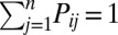and for any i. We assume that the union of - and -associated graphs is strongly connected; namely the infection can spread to any community along either network.

Disease onset is determined by the instability of the disease-free equilibrium (, for all i). If the communities were isolated (no hydrological or mobility connections), the onset condition in each community (13) would require that the local basic reproduction number

where γ is the recovery rate, and μ and α are, respectively, human baseline and disease-induced mortality rates. The connection with more traditional derivations of local values of for classic SIR models is reported in SI Text. Note that various versions of SIR-like local models would command different expressions of , accounting for parameters of the relevant mechanisms (e.g., ref. 28). For the spatially connected system, instead, onset in the metacommunity does not correspond to one or more local reproduction numbers .

Technically, our approach is similar to that of the next-generation matrix (NGM) (29–31), which has been used for compartmental models rather than spatially explicit ones. Both methods are based on dominant eigenvalue analysis (32). More specifically, however, we use a bifurcation analysis (33) to determine how the eigenvalues of the Jacobian at vary with the model parameters (Materials and Methods). As the system is positive and is characterized by null values of and , the bifurcation can occur only via an exchange of stability; i.e., the disease-free equilibrium switches from stable node to saddle through a transcritical bifurcation (the Jacobian has one zero eigenvalue).

Define and introduce the diagonal matrices , , , , and (whose diagonals consist of parameters , , , , and with , respectively). is also diagonal with elements equal to ; thus, . The bifurcation corresponds to

where is the (-dimensional) identity matrix and

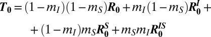is a transmission matrix accounting for different probabilities of movement. , , and are matrices that correspond, respectively, to metacommunities with (i) infectives only, (ii) susceptibles only, or (iii) both infectives and susceptibles being mobile. thus depends on mobility through the terms (movement to a community), (movement from a community), and (movement to and from) (Materials and Methods).

Equivalent to Eq. 1 is that the dominant eigenvalue of the generalized reproduction matrix

equals unity. Our main result is therefore that the onset of the disease can be triggered whenever switches from being less than to being larger than 1; namely

is the sum of two matrices, one depending (linearly) on the hydrological matrix and the other (nonlinearly) on the human mobility matrix . Therefore, the two networks interplay in a complex manner to determine disease insurgence and spread.

The geographical distribution of disease insurgence can be linked to the dominant eigenvector of (SI Text). When is slightly larger than unity and no other eigenvalue has modulus , is a saddle and the dominant eigenvector corresponds to the unique unstable direction in the state space along which the system orbit will diverge from the equilibrium. Once the eigenvector is suitably projected onto the subspace of infectives and normalized, its n components are the relative proportions of the infectives in the n communities (SI Text). Whenever the dominant eigenvalue is sufficiently larger than one, there may be other eigenvalues of with modulus and more than one unstable direction of . However, after a short-term transient due to initial conditions, the disease will mainly propagate to the nodes corresponding to the largest components of the dominant eigenvector. These communities are those where the number of infectives will be highest during the onset and will thus act as the main foci of the disease.

Case Studies

Our approach is applied to the cholera epidemic that struck Haiti in 2010 and is still ongoing (details in SI Text). We use Haiti epidemiological data from November 2010 to May 2011 (Fig. 1 A and B) and a model (based on a network of 366 hydrologic/demographic entities, SI Text) derived from the reassessment (6) of the disease unfolding. Attractivity of a certain destination site is supposed to be given by a constrained gravity model (34),

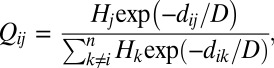Fig. 1.

Data and model predictions of Haiti epidemic. (A) Total incidence data (weekly cases) from November 2010 to May 2011. (B) Fine-grained spatial distribution of recorded cases cumulated during the onset phase of the epidemic (defined as period from beginning to peak, gray area in A). (C) Comparison of coarse-grained data (department level, labels as in A, Inset) on spatial distributions of cumulated cases (gray bars, onset phase; black bars, whole period) vs. predictions based on the dominant eigenvector (white bars). = coefficient of determination for the onset phase = 0.81, = coefficient of determination for the whole period = 0.90. (D) Sensitivity to parameter variations of the dominant eigenvalue of G₀. The dotted horizontal line indicates the value below which the disease cannot start. (E) Fine-grained spatial distribution as predicted by dominant eigenvector (SI Text). = 0.92, = 0.95. (F) Sensitivity to parameter variations of correlations between spatial distribution as predicted by dominant eigenvector and actual spatial distribution of cumulated cases (gray, onset phase; black, whole period). Parameter values and details are in SI Text.

where is the distance between node i and node j and D is the average travel distance. Results of the analysis are reported in Fig. 1 C–F. In the Haitian case is practically insensitive to changes in pathogen movement rate l and average mobility distance D and to increases of the human mobility rate m (Fig. 1D), whereas it is quite sensitive to variations of the exposure and contamination rates β and p, of the pathogen mortality rate , and of the recovery rate (which is the largest component of parameter ϕ). Therefore, an effective way to prevent the onset of cholera would have been to implement sanitation measures to decrease the exposure (or contamination) rate by more than 40%. The alternative would have been to increase the rate of recovery by more than 50% via, e.g., the use of antibiotics, a measure that is not recommended, however, on a massive scale (35). The dominant eigenvector is a good indicator of the spatial distribution of recorded cases at both the coarse administrative level (10 departments, Fig. 1C) and the fine-grained scale (1-km² population pixels, Fig. 1E), as demonstrated by the corresponding coefficients of determination (Fig. 1 legend). A sensitivity analysis has been run to determine how the predictive ability of the dominant eigenvector and the value of change with parameter variations. The coefficients of determination (Fig. 1F) exceed 75% even for variations as high as 50%, thus indicating robustness in the prediction of the spatial pattern.

The Haitian study was purely retrospective. We attempt a real-time predictive use for another monitored case of cholera epidemic (Thukela river basin in KwaZulu-Natal, South Africa, which was struck by cholera in 2000) (Fig. 2 A and B). The structure of the water network (287 nodes) is borrowed from a previous work (9). Model parameters have been estimated via Markov chain Monte Carlo sampling (36), using only the first weeks of epidemiological records as calibration data (Fig. 2A and SI Text). The results are reported in Fig. 2 C–F. The dominant eigenvector (associated to ) is a good indicator of the spatial patterns of disease spread (Fig. 2C), with coefficients of determination for disease onset (gray area in Fig. 2A) and for the epidemic course in 2000–2001. On the contrary, the local reproduction number in excess of one is neither necessary nor sufficient to pinpoint the ensuing epidemic in a spatially connected system. Fig. 2D, in fact, shows a map of the local reproduction numbers at the onset of the epidemic that can be contrasted with the spatial distribution of infection cases in excess of 10 (Fig. 2E). Strikingly, the comparison shows that several regions where still have disease because they are connected to other infected areas. Furthermore, a correlation analysis (details in SI Text) between the number of cases and the local reproduction numbers reveals that the distribution of has a much lower explanatory power than the dominant eigenvector of . Similar results hold for the correlation with the local population sizes and the fraction of households without piped water or toilet facilities, as well as for the related model parameters (exposure probabilities and contamination rates ; SI Text). Their coefficients of determination cannot compete with those resulting from the eigenvector analysis, thus suggesting that not only local living conditions but also pathogen transport (along waterways and induced by human mobility) must be properly taken into account to understand the formation of the spatial patterns of disease spread.

Fig. 2.

Data and model predictions of cholera epidemic along the Thukela river network (A, Inset). (A) Total incidence data (weekly cases) from October 2000 to July 2001. Dotted lines mark the model calibration window. (B) Normalized spatial distribution of recorded cases cumulated during the epidemic onset phase (gray in A). (C) Spatial distribution of cases as predicted by the dominant eigenvector. (D) Spatial distribution of local basic reproduction numbers (details in SI Text). Locations in red (blue) are characterized by (). (E) Cholera cases (as in B). Red (blue) dots indicate communities with more (less) than 10 reported cases during disease onset. (F) Sensitivity to parameter variations of coefficients of determination and (defined in Fig. 1). Parameter values and additional details are in SI Text.

A sensitivity analysis of the Thukela model (Fig. 2F) shows that the dominant eigenvector is quite a robust spatial indicator of disease incidence. Performances are lower than for the Haiti case study, in which, however, model parameters were calibrated using the whole epidemiological dataset. The dominant eigenvector of , as calculated at the end of initial calibration, is not only a good indicator, but also a satisfactory predictor of the disease spatial distribution in the months following the calibration’s end. In fact, of the eigenvector components vs. the fractions of cumulative cases from the end of the calibration window to the epidemic peak is 0.91, whereas it is 0.84 if calculated against the cases from the end of calibration to epidemic fading.

Metapopulation Networks

More insight derives from exploring complex theoretical landscapes with different characteristics of river basin network, population distribution, and human mobility. To this end, we construct abstract hydrological networks endowed with a realistic topology, the Peano networks (37–39), which are deterministic fractals (40) whose scaling topology and metrics have been solved analytically (41) (SI Text). We study both the spatially homogeneous case (all the site-dependent parameters are identical and so are all the ) and the more realistic one in which the population of different communities is distributed according to Zipf’s law (42) (SI Text), mobility is gravity-like, and water volumes are proportional to . Fig. 3 A and B shows the parameter combinations corresponding to disease onset for the homogeneous case. The higher the values are of either l ( is the average residence time of pathogens in each node) or the downstream transport bias b (proportional to stream velocity; SI Text), the higher the local reproduction number must be for an epidemic to be possibly triggered (or triggered with high probability in the case of inhomogeneous population distributions, Fig. 3C). Conversely, for low values of l and b the disease can start even if all the are smaller than unity. We term this phenomenon a locally subthreshold epidemic as was done for compartmental models (43). In fact, when l, , , the local onset conditions () are neither necessary nor sufficient for disease outbreak. Human mobility can remarkably favor disease onset, especially if large population shares move (high m) over either intermediate (homogeneous population, Fig. 3B) or short (Zipf-like distribution, Fig. 3D) distances D. The analysis can be extended to different mobility models based on small-world and scale-free graphs (SI Text). The predictive ability of the dominant eigenvector against the spatial distribution of cases for both homogeneous and Zipf-like population distributions is shown in SI Text. It is very good at disease emergence and during the onset phase, whereas it usually decreases as the epidemic outbreak unfolds (homogeneous population distribution, for disease emergence; for the onset phase; for the whole epidemic course; and Zipf-like population distribution, , , ). This negative trend is especially apparent for the homogeneous case, whereas it is much less evident for Zipf-like population distributions, suggesting that population heterogeneity may play an important role in the definition of long-term spatial patterns of epidemic spread.

Fig. 3.

Onset conditions of a waterborne disease epidemic in a Peano network. (A) Effects of hydrological transport parameters for different local reproductive numbers (labels of isolines) in a homogeneous population. Epidemics can start for combinations lying on the left of the curves with , whereas subthreshold epidemics (gray shading) can be triggered for combinations lying in between the relevant isolines. (B) Same as A for human mobility parameters. Epidemics can start for combinations lying on the right of the isolines. (C) As in A, with and Zipf-like population distribution. Different colors code the fraction of realizations (different population distributions) for which onset conditions are met (SI Text). (D) As in C, with reference to mobility parameters. Other parameter values: , , , (A and C), (A and C), (B and D), and (B and D).

Conclusion

We have derived an epidemiological matrix accounting for both hydrological transport and human mobility. Its dominant eigenvalue is the generalized reproduction number controlling the onset of waterborne disease whereas the dominant eigenvector well characterizes the geography of disease insurgence. Despite the simplicity of the model, the method not only is successful from a theoretical viewpoint, but also proves valid as a tool for analyzing real epidemics (Haiti and KwaZulu-Natal) and inspiring appropriate control measures and sanitation actions, which are the subject of ongoing debate (44, 45). In particular, the model is a good compromise between traditional space-homogeneous approaches (13) and individual-based simulation (5), thus coupling realism with a sufficiently simple structure that allows statistically significant tuning of a few relevant parameters. Spatially explicit data, now widely available, can be easily incorporated into the transmission matrices to describe real landscapes as networks of any complexity, ranging from a few to hundreds of nodes. Obviously, it should be remarked that the approach is valid to study just the onset conditions and cannot be extrapolated to draw conclusions about the long-term fate of waterborne disease. This requires the further inclusion of other fundamental determinants such as immunity loss (6) and seasonal and interannual variations of hydrological conditions (46).

The model can be generalized in many important ways. Including different age classes of human hosts (47), spatial heterogeneity of pathogen ecology (48, 49), and competition between pathogen strains (50) can add further realism to the methodology. Although not easy, expressions for the reproduction matrix can be obtained even for these cases. Our methodology, based on dominant eigenvalue and eigenvector analysis (32) coupled with georeferenced data assimilation, will provide, in our opinion, a valuable and reasonably simple approach for predicting the spatiotemporal epidemic course of waterborne disease outbreaks.

Materials and Methods

Local Epidemic Model.

Epidemiological dynamics of susceptibles and infected/infectives in the ith community, with , and transport of pathogens (represented by their concentrations ) over the networks are described by the following set of ordinary differential equations (t is time):

The evolution of susceptibles (first equation) is a balance between population demography and infections due to contact with a pathogen. The host population, if uninfected, is at demographic equilibrium (the size of the ith local community), with μ being the baseline mortality rate of humans. The parameter is the site-dependent rate of exposure to contaminated water, and (dose-response function) is the probability of becoming infected due to exposure to concentration of pathogens. In accordance with much literature on cholera (13), we use the hyperbolic and saturating function (K is the half-saturation constant). The dynamics of infectives (second equation) are a balance between newly infected individuals and losses due to recovery or natural/pathogen-induced mortality, with γ and α being recovery and disease-induced mortality rates, respectively. The dynamics of recovered individuals are neglected, because waterborne diseases confer at least temporary immunity and its loss neither determines conditions for disease onset nor affects its evolution in the immediate development following the epidemic peak. The dynamics of free-living pathogens concentration (third equation) assume that bacteria or protozoa are released in water (e.g., excreted) by infective individuals and immediately diluted in a well-mixed local water reservoir of volume at a site-dependent rate . Free-living pathogens are also assumed to die at a constant, site-independent rate . Regarding the hydrological transport, the spread of pathogens over the river network is described as a biased random-walk process on an oriented graph (9). Here, we assume that pathogens can move at a rate l from node i to node j of the hydrological network with a probability . The rate depends on both downstream advection and other possible pathogen transport pathways along the hydrological network, e.g., short-range distribution of water for consumption or irrigation or bacterial attachment to phyto- and zooplankton. Possible topological structures for the hydrological network range from simple one-dimensional lattices to realistic mathematical characterizations of existing river networks. The nodes of the human mobility network are assumed to correspond to those of the hydrological layer, whereas edges are defined by connections among communities. We also assume that susceptible and infective individuals can undertake short-term trips from the communities where they live toward other settlements. While traveling or commuting, susceptible individuals can be exposed to pathogens and return as infected carriers to the settlement where they usually live. Similarly, infected hosts can disseminate the disease away from their home community. In many cases infected individuals are asymptomatic and thus are not barred, or are only partially barred, from their usual activities by the presence of the pathogen in their intestine. Human mobility patterns are defined according to a connection matrix in which individuals leave their original node (say i) with an infection-dependent probability (respectively for susceptibles and for infectives, usually with ), reach their target location (say j) with a probability , and then come back to node i. Topological and transition probability structures for human mobility networks used in epidemiology can be based on suitable measures of node-to-node distance like in gravity models (34); on the actual transportation network; or on models based on conceptually different interactions, such as Erdős–Rényi random graphs (51), scale-free networks (52), small-world–like graphs (53), and radiation models (54).

Derivation of Onset Conditions.

To analyze stability, we consider the Jacobian of the linearized system evaluated at the disease-free equilibrium ₀ (, for all i), which is given by

where

Note that the variables for pathogen have been scaled as . Because of its block-triangular structure, the Jacobian has obviously n eigenvalues equal to ; therefore, instability is determined by the eigenvalues of the block matrix

is a proper Metzler matrix (55); namely its off-diagonal entries are all nonnegative and at least one diagonal entry is negative. Thus its eigenvalue with maximal real part (dominant eigenvalue) is real. If the union of the graphs associated with matrices and is strongly connected, then the graph associated with is also strongly connected. Therefore one can apply the Perron–Frobenius theorem (56) for irreducible matrices and state that the dominant eigenvalue is a simple real root of the characteristic polynomial. The condition for the transcritical bifurcation of the disease-free equilibrium is that the dominant eigenvalue crosses the imaginary axis at zero; namely, the determinant of is zero (33). Actually, when the disease-free equilibrium is stable, all the eigenvalues have negative real parts and is positive because is a matrix of order . So the disease-free equilibrium becomes unstable when switches from positive to negative or equivalently the dominant eigenvalue becomes zero.

As obviously commutes with any matrix, we have (ref. 57 and SI Text)

Because , , and are diagonal, thus commuting, matrices, we can state that and rework the determinant of (SI Text). The condition is thus given by

In addition to the matrix we can now introduce three other matrices of reproduction numbers; namely,

corresponding to metacommunities with infectives only being mobile, susceptibles only being mobile, and both infectives and susceptibles being mobile, respectively. If we account for the different probabilities of movement in the metacommunity, we can define a transmission matrix averaged over nonmobile individuals, mobile infectives, and mobile susceptibles as

Therefore, the bifurcation of the disease-free equilibrium corresponds to the condition

Equivalently, the dominant eigenvalue of the matrix

which is a convex combination of and , must equal unity. Actually, the disease-free equilibrium switches from being stable to being a saddle, thus triggering the start of the disease, whenever the dominant eigenvalue of switches from positive to negative and hence whenever switches from being less than 1 to being larger than 1.

References

- 1.World Health Organization . The Global Burden of Disease: 2004 Update. Geneva: WHO; 2008. [Google Scholar]
- 2.Bertuzzo E, et al. Prediction of the spatial evolution and effects of control measures for the unfolding Haiti cholera outbreak. Geophys Res Lett. 2011;38:L06403. [Google Scholar]
- 3.Mari L, et al. Modelling cholera epidemics: The role of waterways, human mobility and sanitation. J R Soc Interface. 2012;9(67):376–388. doi: 10.1098/rsif.2011.0304. [DOI] [PMC free article] [PubMed] [Google Scholar]
- 4.Tuite AR, et al. Cholera epidemic in Haiti, 2010: Using a transmission model to explain spatial spread of disease and identify optimal control interventions. Ann Intern Med. 2011;154(9):593–601. doi: 10.7326/0003-4819-154-9-201105030-00334. [DOI] [PubMed] [Google Scholar]
- 5.Chao DL, Halloran ME, Longini IM., Jr Vaccination strategies for epidemic cholera in Haiti with implications for the developing world. Proc Natl Acad Sci USA. 2011;108(17):7081–7085. doi: 10.1073/pnas.1102149108. [DOI] [PMC free article] [PubMed] [Google Scholar]
- 6.Rinaldo A, et al. Reassessment of the 2010–2011 Haiti cholera outbreak and multi-season projections via inclusion of rainfall and waning immunity. Proc Natl Acad Sci USA. 2012;109:6602–6607. doi: 10.1073/pnas.1203333109. [DOI] [PMC free article] [PubMed] [Google Scholar]
- 7.Mukandavire Z, et al. Estimating the reproductive numbers for the 2008-2009 cholera outbreaks in Zimbabwe. Proc Natl Acad Sci USA. 2011;108(21):8767–8772. doi: 10.1073/pnas.1019712108. [DOI] [PMC free article] [PubMed] [Google Scholar]
- 8.Rohani P, Earn DJ, Grenfell BT. Opposite patterns of synchrony in sympatric disease metapopulations. Science. 1999;286(5441):968–971. doi: 10.1126/science.286.5441.968. [DOI] [PubMed] [Google Scholar]
- 9.Bertuzzo E, et al. On the space-time evolution of a cholera epidemic. Water Resour Res. 2008;44:W01424. [Google Scholar]
- 10.Bertuzzo E, Casagrandi R, Gatto M, Rodriguez-Iturbe I, Rinaldo A. On spatially explicit models of cholera epidemics. J R Soc Interface. 2010;7(43):321–333. doi: 10.1098/rsif.2009.0204. [DOI] [PMC free article] [PubMed] [Google Scholar]
- 11.Pitzer VE, et al. Demographic variability, vaccination, and the spatiotemporal dynamics of rotavirus epidemics. Science. 2009;325(5938):290–294. doi: 10.1126/science.1172330. [DOI] [PMC free article] [PubMed] [Google Scholar]
- 12.Capasso V, Paveri-Fontana SL. A mathematical model for the 1973 cholera epidemic in the European Mediterranean region. Rev Epidemiol Sante Publique. 1979;27(2):121–132. [PubMed] [Google Scholar]
- 13.Codeço CT. Endemic and epidemic dynamics of cholera: The role of the aquatic reservoir. BMC Infect Dis. 2001;1:1. doi: 10.1186/1471-2334-1-1. [DOI] [PMC free article] [PubMed] [Google Scholar]
- 14.Anderson R, May R. Infectious Diseases of Humans: Dynamics and Control. Oxford: Oxford Univ Press; 1991. [Google Scholar]
- 15.Hartley DM, Morris JG, Jr, Smith DL. Hyperinfectivity: A critical element in the ability of V. cholerae to cause epidemics? PLoS Med. 2006;3(1):e7. doi: 10.1371/journal.pmed.0030007. [DOI] [PMC free article] [PubMed] [Google Scholar]
- 16.Jensen MA, Faruque SM, Mekalanos JJ, Levin BR. Modeling the role of bacteriophage in the control of cholera outbreaks. Proc Natl Acad Sci USA. 2006;103(12):4652–4657. doi: 10.1073/pnas.0600166103. [DOI] [PMC free article] [PubMed] [Google Scholar]
- 17.Colwell RR. Global climate and infectious disease: The cholera paradigm. Science. 1996;274(5295):2025–2031. doi: 10.1126/science.274.5295.2025. [DOI] [PubMed] [Google Scholar]
- 18.Pascual M, Bouma MJ, Dobson AP. Cholera and climate: Revisiting the quantitative evidence. Microbes Infect. 2002;4(2):237–245. doi: 10.1016/s1286-4579(01)01533-7. [DOI] [PubMed] [Google Scholar]
- 19.Lipp EK, Huq A, Colwell RR. Effects of global climate on infectious disease: The cholera model. Clin Microbiol Rev. 2002;15(4):757–770. doi: 10.1128/CMR.15.4.757-770.2002. [DOI] [PMC free article] [PubMed] [Google Scholar]
- 20.Koelle K, Rodó X, Pascual M, Yunus M, Mostafa G. Refractory periods and climate forcing in cholera dynamics. Nature. 2005;436(7051):696–700. doi: 10.1038/nature03820. [DOI] [PubMed] [Google Scholar]
- 21.Reiner RC, Jr, et al. Highly localized sensitivity to climate forcing drives endemic cholera in a megacity. Proc Natl Acad Sci USA. 2012;109(6):2033–2036. doi: 10.1073/pnas.1108438109. [DOI] [PMC free article] [PubMed] [Google Scholar]
- 22.Righetto L, et al. The role of aquatic reservoir fluctuations in long-term cholera patterns. Epidemics. 2012;4(1):33–42. doi: 10.1016/j.epidem.2011.11.002. [DOI] [PubMed] [Google Scholar]
- 23.World Health Organization 2010. Prevention and Control of Cholera Outbreaks: WHO Policy and Recommendations, Technical Report (WHO Global Task Force on Cholera Control, Geneva, Switzerland)
- 24.Guerrant R. The global problem of amebiasis: Current status, research needs, and opportunities for progress. Rev Infect Dis. 1986;8:218–227. doi: 10.1093/clinids/8.2.218. [DOI] [PubMed] [Google Scholar]
- 25.Righetto L, et al. Modelling human movement in cholera spreading along fluvial systems. Ecohydrology. 2011;4:49–55. [Google Scholar]
- 26.Mari L, et al. On the role of human mobility in the spread of cholera epidemics: Towards an epidemiological movement ecology. Ecohydrology. 2012;5(5):531–540. [Google Scholar]
- 27.Rodriguez-Iturbe I, Rinaldo A. Fractal River Basins: Chance and Self-Organization. New York: Cambridge Univ Press; 1997. [Google Scholar]
- 28.Grad YH, Miller JC, Lipsitch M. Cholera modeling: Challenges to quantitative analysis and predicting the impact of interventions. Epidemiology. 2012;23(4):523–530. doi: 10.1097/EDE.0b013e3182572581. [DOI] [PMC free article] [PubMed] [Google Scholar]
- 29.Diekmann O, Heesterbeek JAP, Roberts MG. The construction of next-generation matrices for compartmental epidemic models. J R Soc Interface. 2010;7(47):873–885. doi: 10.1098/rsif.2009.0386. [DOI] [PMC free article] [PubMed] [Google Scholar]
- 30.Roberts MG, Heesterbeek JAP. A new method for estimating the effort required to control an infectious disease. Proc Biol Sci. 2003;270(1522):1359–1364. doi: 10.1098/rspb.2003.2339. [DOI] [PMC free article] [PubMed] [Google Scholar]
- 31.Lopez LF, Coutinho FAB, Burattini MN, Massad E. Threshold conditions for infection persistence in complex host-vectors interactions. C R Biol. 2002;325(11):1073–1084. doi: 10.1016/s1631-0691(02)01534-2. [DOI] [PubMed] [Google Scholar]
-
32.Diekmann O, Heesterbeek JA, Metz JA. On the definition and the computation of the basic reproduction ratio
in models for infectious diseases in heterogeneous populations. J Math Biol. 1990;28(4):365–382. doi: 10.1007/BF00178324. [DOI] [PubMed] [Google Scholar]
- 33.Kuznetsov Y. Elements of Applied Bifurcation Theory. New York: Springer; 1995. [Google Scholar]
- 34.Erlander S, Stewart NF. The Gravity Model in Transportation Analysis – Theory and Extensions. Zeist, The Netherlands: VSP Books; 1990. [Google Scholar]
- 35.Nelson EJ, Nelson DS, Salam MA, Sack DA. Antibiotics for both moderate and severe cholera. N Engl J Med. 2011;364(1):5–7. doi: 10.1056/NEJMp1013771. [DOI] [PubMed] [Google Scholar]
- 36.Gilks WR, Richardson S, Spiegelharter DJ. Markov Chain Monte Carlo in Practice. New York: Chapman & Hall; 1995. [Google Scholar]
- 37.Peano G. Sur une courbe qui remplit toute une air plane [On an area-filling curve] Math. Ann. 1890;36:157–160. [Google Scholar]
- 38.Campos D, Fort J, Méndez V. Transport on fractal river networks: Application to migration fronts. Theor Popul Biol. 2006;69(1):88–93. doi: 10.1016/j.tpb.2005.09.001. [DOI] [PubMed] [Google Scholar]
- 39.Bertuzzo E, Maritan A, Gatto M, Rodriguez-Iturbe I, Rinaldo A. River networks and ecological corridors: Reactive transport on fractals, migration fronts, hydrochory. Water Resour Res. 2007;43:W04419. [Google Scholar]
- 40.Mandelbrot B. The Fractal Geometry of Nature. New York: Freeman; 1983. [Google Scholar]
- 41.Marani A, Rigon R, Rinaldo A. A note on fractal channel networks. Water Resour Res. 1991;27:3041–3049. [Google Scholar]
- 42.Zipf GK. Human Behavior and the Principle of Least Effort: An Introduction to Human Ecology. Cambridge, MA: Addison-Wesley; 1949. [Google Scholar]
- 43.van den Driessche P, Watmough J. Reproduction numbers and sub-threshold endemic equilibria for compartmental models of disease transmission. Math Biosci. 2002;180:29–48. doi: 10.1016/s0025-5564(02)00108-6. [DOI] [PubMed] [Google Scholar]
- 44.Farmer P, et al. Meeting cholera’s challenge to Haiti and the world: A joint statement on cholera prevention and care. PLoS Negl Trop Dis. 2011;5(5):e1145. doi: 10.1371/journal.pntd.0001145. [DOI] [PMC free article] [PubMed] [Google Scholar]
- 45.Walton DA, Ivers LC. Responding to cholera in post-earthquake Haiti. N Engl J Med. 2011;364(1):3–5. doi: 10.1056/NEJMp1012997. [DOI] [PubMed] [Google Scholar]
- 46.Bertuzzo E, et al. Hydroclimatology of dual-peak cholera epidemics: Inferences from a spatially explicit model. Geophys Res Lett. 2012;39:L05403. [Google Scholar]
- 47.Siddique AK, et al. Epidemiology of rotavirus and cholera in children aged less than five years in rural Bangladesh. J Health Popul Nutr. 2011;29(1):1–8. doi: 10.3329/jhpn.v29i1.7560. [DOI] [PMC free article] [PubMed] [Google Scholar]
- 48.Vezzulli L, Pruzzo C, Huq A, Colwell R. Environmental reservoirs of Vibrio cholerae and their role in cholera. Environ Microbiol Rep. 2010;2:27–33. doi: 10.1111/j.1758-2229.2009.00128.x. [DOI] [PubMed] [Google Scholar]
- 49.Lara R, et al. Vibrio cholerae in waters of the Sunderban mangrove: Relationship with biogeochemical parameters and chitin in seston size fractions. Wetlands Ecol Manage. 2011;19:109–119. [Google Scholar]
- 50.Faruque SM, et al. Pathogenic potential of environmental Vibrio cholerae strains carrying genetic variants of the toxin-coregulated pilus pathogenicity island. Infect Immun. 2003;71(2):1020–1025. doi: 10.1128/IAI.71.2.1020-1025.2003. [DOI] [PMC free article] [PubMed] [Google Scholar]
- 51.Erdős P, Rényi A. On random graphs. Publicationes Mathematicae. 1959;6:290–297. [Google Scholar]
- 52.Albert R, Barabási A-L. Statistical mechanics of complex networks. Rev Mod Phys. 2002;74:4797. [Google Scholar]
- 53.Watts DJ, Strogatz SH. Collective dynamics of ‘small-world’ networks. Nature. 1998;393(6684):440–442. doi: 10.1038/30918. [DOI] [PubMed] [Google Scholar]
- 54.Simini F, González MC, Maritan A, Barabási A-L. A universal model for mobility and migration patterns. Nature. 2012;484(7392):96–100. doi: 10.1038/nature10856. [DOI] [PubMed] [Google Scholar]
- 55.Farina L, Rinaldi S. Positive Linear Systems: Theory and Applications. New York: Wiley Interscience; 2000. [Google Scholar]
- 56.Gantmacher F. Theory of Matrices. Providence, RI: AMS Chelsea Publishing; 1959. [Google Scholar]
- 57.Silvester J. Determinants of block matrices. Math Gazette. 2000;84:460–467. [Google Scholar]
Associated Data
This section collects any data citations, data availability statements, or supplementary materials included in this article.