Hierarchical Model of Fibrillar Collagen Organization for Interpreting the Second-Order Susceptibility Tensors in Biological Tissue

Abstract

The second-order nonlinear polarization properties of fibrillar collagen in various rat tissues (vertebrae, tibia, tail tendon, dermis, and cornea) are investigated with polarization-dependent second-harmonic generation (P-SHG) microscopy. Three parameters are extracted: the second-order susceptibility ratio, R = ${\chi }_{ZZZ}^{{\left(2\right)}^{\prime }}/{\chi }_{ZXX}^{{\left(2\right)}^{\prime }}$; a measure of the fibril distribution asymmetry, |A|; and the weighted-average fibril orientation, 〈δ〉. A hierarchical organizational model of fibrillar collagen is developed to interpret the second-harmonic generation polarization properties. Highlights of the model include: collagen type (e.g., type-I, type-II), fibril internal structure (e.g., straight, constant-tilt), and fibril architecture (e.g., parallel fibers, intertwined, lamellae). Quantifiable differences in internal structure and architecture of the fibrils are observed. Occurrence histograms of R and |A| distinguished parallel from nonparallel fibril distributions. Parallel distributions possessed low parameter values and variability, whereas nonparallel distributions displayed an increase in values and variability. From the P-SHG parameters of vertebrae tissue, a three-dimensional reconstruction of lamellae of intervertebral disk is presented.

Introduction

Tissue architecture and function are intimately linked with the organization of collagen. Through alterations to the organization of collagen, forces can be transferred in tendon, pressures can be resisted in bone, shocks can be absorbed in cartilage, and light can be better focused with cornea (1–4). Collagen even provides the scaffolding of blood vessels and most organs (2,4). Therefore, it should come of little surprise that over the last half century, systems of collagen have been actively studied using an assortment of chemical and physical methods (1–6).

The collagen molecule is composed of three left-handed helical chains, which assemble to form a triple-helix structure (5–7). Each helical chain is constructed from a sequence of amino acids, where every third amino acid is glycine (GLY). The collagen triple-helices then organize into larger fibrils and, ultimately, fibers by way of cross-linking molecules. The most common fibrillar collagen types (type-I and -II) are genetically distinct and composed of different sequences of amino acids. The relative variation in amino-acid composition between type-I and -II is minimal (<±2%) and equivalent to the interchain variation of type-I (2,3,8), reasonably suggesting the two types, on average, are comprised of a similar collagen triple-helix.

With sufficient knowledge of the elementary structure of collagen fibrils, focus has shifted to investigating dynamic changes to the organization of collagen and its effect on the functional and structural integrity of tissue (9–13). One method, promising to be a valuable tool for quantifying organizational changes in collagen, is polarization-dependent second-harmonic generation (P-SHG) microscopy (14–19). This technique has many attractive characteristics including submicron resolution and label-free structural specificity (20,21). For second-harmonic to be generated, inversion symmetry must be absent from the molecules and material (22). The spatial symmetry of the system and the orientation of the incident field polarization affect the efficiency of the conversion process. The propensity of a system to generate second-harmonic is commonly described in terms of its microscopic and macroscopic components—the first hyperpolarizability tensor and the second-order nonlinear susceptibility tensor, respectively (23).

The hyperpolarizability contains spatial symmetry information regarding the molecules comprising the material of interest. The second-order nonlinear susceptibility is the volume-averaged molecular hyperpolarizability, with local field corrections. The second-order nonlinear susceptibility depends on the molecular composition within the focal volume, as well as the spatial organization of the macromolecular units. Therefore, when SHG polarization properties of collagen are observed to differ in various biological tissues, one must remember it is not necessarily only the composition of the collagen macromolecules that are varying but possibly the organization of the macromolecules as well. The susceptibility tensor contains 27 elements, though certain spatial symmetries reduce the number of unique elements. For example, cylindrical symmetry (C_6ν) is often employed for collagen, reducing the number of nonvanishing independent elements to three (14–19,24–26). Originally, Roth and Freund (27) studied and quantified collagen properties, with P-SHG. The P-SHG experiments involve varying the incident polarization and measuring the second-harmonic intensity. Additionally, an analyzer may be used to collect second-harmonic at two orthogonal orientations (17,27). With knowledge of the SHG polarization dependence, ratios of the second-order susceptibility elements may be determined.

The aim of this work is to provide a consistent framework to understand and interpret the susceptibility ratios of fibrillar collagen in biological tissues. An extension of the original experimental method used by Roth and Freund (27), termed “polarization-in, polarization-out” (PIPO), will be presented; the theory of a hierarchical model of collagen organization for interpreting collagen susceptibility ratios will be developed; and distributions of collagen susceptibility ratios measured in various tissues will be interpreted in light of the developed model.

Theoretical Background

To meaningfully quantify SHG from systems of collagen with PIPO microscopy, correct interpretation of the susceptibility ratios is essential. To interpret the susceptibility ratios, in terms of the spatial arrangement of collagen, review of the hierarchical organization of collagen is useful.

Organization of individual collagen fibrils

The lowest level of organization after the triple-helix is the collagen fibril. Two fibril models are considered here: a straight fibril and a constant-tilt fibril (1). The straight fibril is self-explanatory, with all the triple-helices aligned along the fibril axis. Straight fibrils are found in rat-tail tendon (1,4). The ${\chi }_{zzz}^{\left(2\right)}/{\chi }_{zxx}^{\left(2\right)}$ ratio of straight fibrils is equal to the average hyperpolarizability ratio, β_zzz/β_zxx, of the collagen triple-helices (28, 29). The fibril coordinate system is defined as xyz, with the z axis corresponding to the fibril axis. Constant-tilt fibrils have been observed in dermis and cornea (1,4,7). This model has the triple-helices wrapping around the fibril axis (i.e., the z axis) at a constant-tilt angle of 16–18°. The ${\chi }_{zzz}^{\left(2\right)}/{\chi }_{zxx}^{\left(2\right)}$ ratio has been shown to be (28)

$$\frac{{\chi }_{zzz}^{\left(2\right)}}{{\chi }_{zxx}^{\left(2\right)}}=\frac{2\left(3+\left(\frac{{\beta }_{zzz}}{{\beta }_{zxx}}-3\right){\text{cos}}^2{\theta }_{t-h}\right)}{\frac{{\beta }_{zzz}}{{\beta }_{zxx}}-1-\left(\frac{{\beta }_{zzz}}{{\beta }_{zxx}}-3\right){\text{cos}}^2{\theta }_{t-h}},$$ (1)

where θ_t–h refers to the constant-tilt angle.

Susceptibility ratio dependence on collagen fibril organization in tissue

With the fibril models established, the organization of the fibrils in tissue must be considered (30). Cartesian coordinates, XYZ, are introduced to describe the laboratory frame, where the tissue section is positioned in the XZ plane (i.e., microscope sample stage) and the wave-vectors orient along the Y axis (see Fig. 1 a). In the simplest case, for each voxel (i.e., focal volume) of the imaged tissue section, a single collagen fibril may be arbitrarily oriented, with the orientation of the fibrils freely varying between imaged voxels. The orientation of collagen fibrils can be defined in the laboratory frame with modified spherical coordinates, α and δ (Fig. 1 a). The angle α is the tilt of the fibril with respect to the XZ plane, whereas δ is the angle between the projection of the fibril onto the XZ plane and the Z axis. The ratios of the second-order susceptibility tensor elements, ${\chi }_{IJK}^{{\left(2\right)}^{\prime }}$, of an arbitrarily oriented fibril are related to the spherical coordinates of the fibril orientation, in the laboratory frame, as follows (see derivations in Appendix A):

$$\frac{{\chi }_{ZZZ}^{{\left(2\right)}^{\prime }}}{{\chi }_{ZXX}^{{\left(2\right)}^{\prime }}}=\frac{\left(\frac{{\chi }_{zzz}^{\left(2\right)}}{{\chi }_{zxx}^{\left(2\right)}}-3\right){\text{cos}}^2\alpha {\text{cos}}^2\delta +3}{\left(\frac{{\chi }_{zzz}^{\left(2\right)}}{{\chi }_{zxx}^{\left(2\right)}}-3\right){\text{cos}}^2\alpha {\text{sin}}^2\delta +1},$$ (2)

$$\frac{{\chi }_{XXX}^{{\left(2\right)}^{\prime }}}{{\chi }_{ZXX}^{{\left(2\right)}^{\prime }}}=\frac{\text{sin}\delta \left[\left(\frac{{\chi }_{zzz}^{\left(2\right)}}{{\chi }_{zxx}^{\left(2\right)}}-3\right){\text{cos}}^2\alpha {\text{sin}}^2\delta +3\right]}{\text{cos}\delta \left[\left(\frac{{\chi }_{zzz}^{\left(2\right)}}{{\chi }_{zxx}^{\left(2\right)}}-3\right){\text{cos}}^2\alpha {\text{sin}}^2\delta +1\right]},$$ (3)

$$\frac{{\chi }_{XZZ}^{{\left(2\right)}^{\prime }}}{{\chi }_{ZXX}^{{\left(2\right)}^{\prime }}}=\frac{\text{sin}\delta \left[\left(\frac{{\chi }_{zzz}^{\left(2\right)}}{{\chi }_{zxx}^{\left(2\right)}}-3\right){\text{cos}}^2\alpha {\text{cos}}^2\delta +1\right]}{\text{cos}\delta \left[\left(\frac{{\chi }_{zzz}^{\left(2\right)}}{{\chi }_{zxx}^{\left(2\right)}}-3\right){\text{cos}}^2\alpha {\text{sin}}^2\delta +1\right]}.$$ (4)

Equations 2–4 assume single fibrils in each voxel. However, in tissue, collagen fibrils may have broad orientation distributions that differ for various tissue types. For the case of multiple fibrils, the volume-weighted average orientation of all collagen fibrils in the voxel must be considered.

Figure 1.

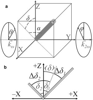
Orientation of fibril(s) in optical setup. (a) Orientation of a collagen fibril is shown in terms of modified spherical coordinates, α and δ, in the laboratory frame, XYZ. The values ${\overrightarrow{k}}_{\omega }$ and ${\overrightarrow{k}}_{2\omega }$ indicate the wave-vectors of the incident and second-harmonic electric fields, respectively. The values θ and φ are the polarizer and analyzer angles with respect to the Z axis. (b) Projection of a distribution of fibrils (e.g., two fibrils) on the XZ plane. The value 〈δ〉 is the weighted-average orientation, Δδ₁ is the difference between δ₁ and 〈δ〉 for fibril 1, and Δδ₂ is the difference between δ₂ and 〈δ〉 for fibril 2.

From Eqs. 2–4, two relevant ratios may be defined for arbitrary distributions of fibrils (e.g., crossed, out-of-plane, interwoven meshwork, etc.). The first ratio, R, is standard for P-SHG experiments (14–19,24–30), whereas a second ratio, A, for the first time, to our knowledge, presented here, provides a measure of the asymmetry of a distribution (see Appendix A),

$$R=\frac{{\chi }_{ZZZ}^{{\left(2\right)}^{\prime }}}{{\chi }_{ZXX}^{{\left(2\right)}^{\prime }}}=\frac{\left(\frac{{\chi }_{zzz}^{\left(2\right)}}{{\chi }_{zxx}^{\left(2\right)}}-3\right)\frac{\langle {\text{cos}}^3\alpha {\text{cos}}^3\Delta \delta \rangle }{\langle \text{cos}\alpha \text{cos}\Delta \delta \rangle }+3}{\left(\frac{{\chi }_{zzz}^{\left(2\right)}}{{\chi }_{zxx}^{\left(2\right)}}-3\right)\left(\frac{\langle {\text{cos}}^3\alpha \text{cos}\Delta \delta \rangle }{\langle \text{cos}\alpha \text{cos}\Delta \delta \rangle }-\frac{\langle {\text{cos}}^3\alpha {\text{cos}}^3\Delta \delta \rangle }{\langle \text{cos}\alpha \text{cos}\Delta \delta \rangle }\right)+1},$$ (5)

$$A=\frac{{\chi }_{XXX}^{{\left(2\right)}^{\prime }}+{\chi }_{XZZ}^{{\left(2\right)}^{\prime }}}{{\chi }_{ZZZ}^{{\left(2\right)}^{\prime }}+{\chi }_{ZXX}^{{\left(2\right)}^{\prime }}}=\frac{\left(\frac{{\chi }_{zzz}^{\left(2\right)}}{{\chi }_{zxx}^{\left(2\right)}}-3\right)\langle {\text{cos}}^3\alpha \text{sin}\Delta \delta \rangle +4\langle \text{cos}\alpha \text{sin}\Delta \delta \rangle }{\left(\frac{{\chi }_{zzz}^{\left(2\right)}}{{\chi }_{zxx}^{\left(2\right)}}-3\right)\langle {\text{cos}}^3\alpha \text{cos}\Delta \delta \rangle +4\langle \text{cos}\alpha \text{cos}\Delta \delta \rangle },$$ (6)

where 〈…〉 indicates the weighted average and Δδ = δ − 〈δ〉 is defined for each fibril (Fig. 1 b). From the measured ratios, the orientation of collagen fibrils present in the tissue can be extracted. For example, from Eqs. 5 and 6, isolating α is achieved by assuming a parallel distribution of collagen fibrils (i.e., Δδ = 0 and α is constant for all fibrils in the distribution), resulting in R and A simplifying to the more traditional case of $R={\chi }_{zzz}^{\left(2\right)}/{\chi }_{zxx}^{\left(2\right)}{\text{cos}}^2\alpha +3{\text{sin}}^2\alpha$ and A = 0.

Intensity dependence of polarization-in, polarization-out SHG microscopy

To gain insight into the general fibril distributions within the microscope focal volume, the relevant second-order susceptibility tensor element ratios must be deduced from polarization-in, polarization-out (PIPO) measurements. Therefore, a general intensity equation for PIPO SHG measurements is derived, with the assumption of Kleinman symmetry (see derivation in Appendix B),

$$I_{2\omega }\propto |\text{sin}\left(\phi +\langle \delta \rangle \right)\left(\frac{{\chi }_{XXX}^{{\left(2\right)}^{\prime }}}{{\chi }_{ZXX}^{{\left(2\right)}^{\prime }}}{\text{sin}}^2\left(\theta +\langle \delta \rangle \right)+\text{sin}2\left(\theta +\langle \delta \rangle \right)+\frac{{\chi }_{XZZ}^{{\left(2\right)}^{\prime }}}{{\chi }_{ZXX}^{{\left(2\right)}^{\prime }}}{\text{cos}}^2\left(\theta +\langle \delta \rangle \right)\right)+{\text{cos}\left(\phi +\langle \delta \rangle \right)\left({\text{sin}}^2\left(\theta +\langle \delta \rangle \right)+\frac{{\chi }_{XZZ}^{{\left(2\right)}^{\prime }}}{{\chi }_{ZXX}^{{\left(2\right)}^{\prime }}}\text{sin}2\left(\theta +\langle \delta \rangle \right)+\frac{{\chi }_{ZZZ}^{{\left(2\right)}^{\prime }}}{{\chi }_{ZXX}^{{\left(2\right)}^{\prime }}}{\text{cos}}^2\left(\theta +\langle \delta \rangle \right)\right)|}^2,$$ (7)

where ${\chi }_{IJK}^{{\left(2\right)}^{\prime }}$ refers to the IJK^th element of the second-order nonlinear susceptibility in the laboratory frame, θ is the angle of the incident polarization with respect to the Z axis, and φ is the angle of the analyzer with respect to the Z axis. Equation 7 assumes birefringence is negligible, which is reasonable for thin sections of tissue. However, if the tissue sample is relatively thick, birefringence must be accounted for (25).

Materials and Methods

PIPO microscope

A multicontrast nonlinear microscope modified for PIPO measurements has been previously described (28,31). Briefly, a linear polarizer (Laser Components, Nashua, NH) and a custom half-wave plate (Comar Optics, Regina, Saskatchewan, Canada) were placed before the excitation objective and a linear polarizer (Laser Components) was introduced in front of the SHG photomultiplier tube (Hamamatsu, Bridgewater, NJ). The microscope was coupled with a custom-built femtosecond Yb:KGd(WO₄)₂ oscillator. The 1028-nm laser provided ∼430-fs pulses at a 14.3-MHz repetition rate (32). A 20× 0.75 NA air objective (Carl Zeiss, Thornwood, NY) was used for focusing the laser beam. A 514 ± 10 nm band-pass filter (Semrock, Rochester, NY) was used for SHG collection. The collagen samples were imaged with ∼30 pJ pulse energy for 50–100 frames at a 2-μs pixel dwell-time forming an image with 128 × 128 pixels. SHG images were collected at 132 sets of excitation and analyzer angles. The half-wave plate was rotated to 11 different evenly spaced excitation angles from −π/2 to π/2 whereas the analyzer was rotated to 11 different evenly spaced angles from −π/2 to π/2 for each excitation angle. References frames, to monitor SHG intensity fluctuations, were imaged every 11 measurements (11 × 12 = 132 sets).

Data analysis

For each 2 × 2 pixel area (approximately the area of the focal spot size), the variation in SHG intensity as a function of θ and φ was fit using Eq. 7 and a custom Levenberg-Marquardt algorithm. Great care must be taken when implementing a Levenberg-Marquardt algorithm to obtain meaningful results, as the process is sensitive to initial conditions and whether the fitting parameters are orthogonal (i.e., no coupling). To test the algorithm, hundreds of simulations of SHG from various collagen distributions were performed using a chirp-z transform method. The method will be described in detail elsewhere (D. Sandkujil, A. E. Tuer, D. Tokarz, J. Sipe, and V. Barzda, unpublished). The optimal algorithm was a two-step process. Initially, ${\chi }_{ZXX}^{{\left(2\right)}^{\prime }}=1$ and ${\chi }_{XXX}^{{\left(2\right)}^{\prime }}={\chi }_{XZZ}^{{\left(2\right)}^{\prime }}=0$, whereas ${\chi }_{ZZZ}^{{\left(2\right)}^{\prime }}$ and 〈δ〉 were fit under various initial conditions, with the optimal values determined by the adjusted-R². This is robust, as ${\chi }_{ZZZ}^{{\left(2\right)}^{\prime }}$ and 〈δ〉 are orthogonal, with ${\chi }_{ZZZ}^{{\left(2\right)}^{\prime }}$ fitting the shape of the peaks in the PIPO plot and 〈δ〉 determining the diagonal peak positions (see Principle Features of PIPO Plots, below, and see Fig. 2). The second step was fitting ${\chi }_{XXX}^{{\left(2\right)}^{\prime }}$ and ${\chi }_{XZZ}^{{\left(2\right)}^{\prime }}$, which can account for asymmetry in the PIPO plot. However, as 〈δ〉 is coupled to ${\chi }_{XXX}^{{\left(2\right)}^{\prime }}$ and ${\chi }_{XZZ}^{{\left(2\right)}^{\prime }}$ (see Eqs. 3 and 4), the additional constraint of minimizing $\left|{\chi }_{XXX}^{{\left(2\right)}^{\prime }}\right|$ and $\left|{\chi }_{XZZ}^{{\left(2\right)}^{\prime }}\right|$ had to be implemented.

Figure 2.

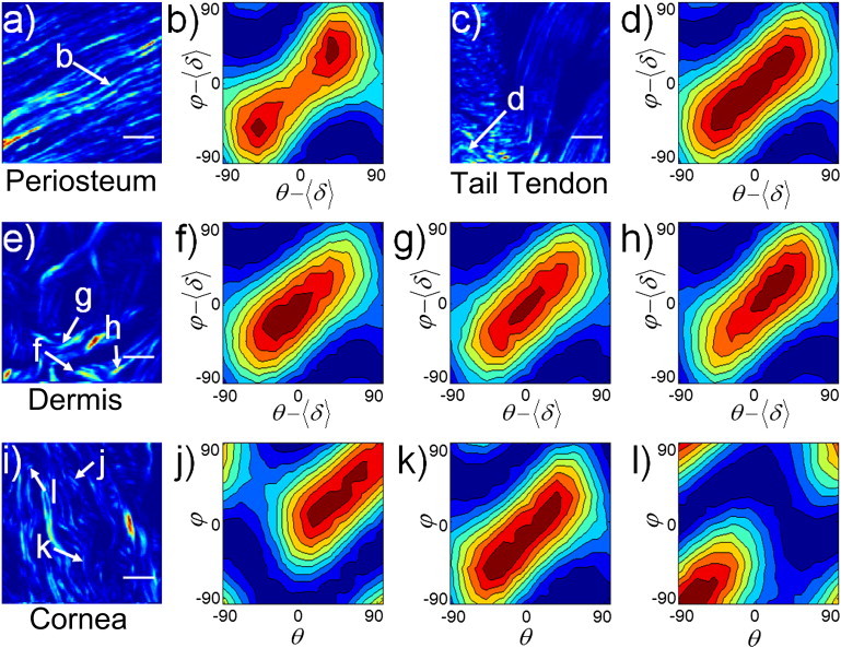
Experimental characteristic PIPO plots. (a, c, e, and i) SHG images of periosteum, rat-tail tendon, dermis, and cornea, respectively. (b, d, f–h, and j–l) PIPO plots of the 2 × 2 pixel arrays indicated on the SHG images (arrows). The scale bar is 10 μm.

From simulations, this additional constraint on the fitting algorithm was found to decouple ${\chi }_{XXX}^{{\left(2\right)}^{\prime }}$ and ${\chi }_{XZZ}^{{\left(2\right)}^{\prime }}$ from the determination of 〈δ〉. The values ${\chi }_{ZZZ}^{{\left(2\right)}^{\prime }}$ and 〈δ〉 of the first step were used as initial parameters with tight bounds (±25%) and the Levenberg-Marquardt algorithm was iterated. If there was appreciable improvement in the fitting (defined as a 1.5% increase in the adjusted-R²) when allowing ${\chi }_{XXX}^{{\left(2\right)}^{\prime }}$ and ${\chi }_{XZZ}^{{\left(2\right)}^{\prime }}$ to be free, then the results of the second step were used; however, if this condition was not met, then the fitting results of the first step were selected. The adjusted-R² goodness-of-fit criterion was deemed suitable as it only increases with the introduction of new parameters, if the improvement is greater than that which would be expected by chance. The process was repeated for each selected area (i.e., 2 × 2 pixel area), if the average maximum signal per pixel was above 20 counts (noise was ∼1 count/pixel). All code was custom-written in MATLAB (The MathWorks, Natick, MA).

Sample preparation: collagen in tissue

The following collagen containing rat tissues were obtained: tail tendon, dermis, cornea, tibia, and vertebrae. The tissues were fixed in 10% neutral buffered formalin and processed into paraffin blocks. The bone containing specimens—tibia and vertebrae—were decalcified using 10% EDTA (ethylenediaminetetraacetic acid) before further processing. Two 4-μm sections were cut, one stained with hematoxylin and eosin (H&E), and the other used for SHG imaging. One sample of rat-tail tendon was left crimped and another was fixed elongated to prevent crimping and maintain the parallel distribution of fibrils.

Results

Principle features of PIPO plots

PIPO microscopy can probe the ultrastructure of fibrillar collagen within the focal volume of the optical setup. With the aim of interpreting the second-order polarization properties of fibrillar collagen, it is informative to visualize P-SHG results, from a 2 × 2 voxel bundle (i.e., pixel area), with PIPO contour plots. For collagen fibrils, a number of characteristic PIPO plots arise from various tissue architectures (Fig. 2). For parallel distributions of type-I collagen fibrils lying in the focal plane, like those observed in the periosteum of a vertebrae section (Fig. 2 a), the PIPO plot reveals a diagonal figure-eight pattern with two equally weighted lobes (Fig. 2 b). The plot corresponds to an R-ratio of ∼1.4 and possesses no appreciable asymmetry (|A| ≈ 0). If a parallel distribution of collagen fibrils is oriented at an angle α to the focal plane (XZ plane), a higher R-ratio results, according to Eq. 5. Indeed for a region of rat-tail tendon sectioned at an angle (Fig. 2 c), the PIPO plot is characteristic of a higher R-ratio (1.8 compared to 1.4) (Fig. 2 d). There also is no appreciable asymmetry. A higher R-ratio may also result if a nonparallel distribution (e.g., lamellae or woven meshwork of fibrils) of multiple fibrils projected on the XZ plane are present in the focal volume. PIPO plots of a rat skin (dermis) section (Fig. 2 e) revealed a higher R-ratio (∼2), where a nonparallel distribution of fibrils is expected (Fig. 2, f–h) (33).

Contrary to the previous two examples, asymmetries are observed in the PIPO plots of dermis (Fig. 2, f–h). Whereas the central PIPO plot has no appreciable asymmetry (Fig. 2 g), the adjacent plots have magnitudes for the |A|-ratio of ∼0.2 (Fig. 2, f and h), with the sign corresponding to the quadrant of the asymmetry (i.e., whether the intensity distribution is skewed to the upper-right quadrant, i.e., positive, or the lower-left quadrant, i.e., negative, of the PIPO plot).

The weighted-average fibril angle, 〈δ〉, shifts the polarizer and analyzer zero positions (see Eq. 7) and thus translates the PIPO intensity patterns along the diagonal, defined by θ = φ. The lamellae of rat cornea were measured to demonstrate the diagonal translation of the intensity pattern (i.e., the shift along θ = φ of the plot) (Fig. 2, i–l). From the translation, the weighted-average orientation of the collagen fibrils projected on to the XZ plane may be extracted as 〈δ〉 (Fig. 2, j–l). The central PIPO plot shows no translation (Fig. 2 k), corresponding to the average fibril orientation being along the laboratory Z axis (Fig. 2 i). Fig. 2, parts j and l, reveal a positive and negative diagonal translation, respectively, corresponding to the orientations of the fibrils observed in the SHG image (Fig. 2 i).

Distribution of PIPO parameters in tissue

With the ability to interpret the PIPO plots and extract relevant parameters, the second-order polarization properties of various rat tissues were investigated (vertebrae, tail tendon, dermis, cornea, and tibia). The dimension of a single pixel in the SHG images is approximately half the lateral resolution of the microscope. Thus a 2 × 2 pixel array (if a pixel array larger than the focal spot size is used on a nonparallel distribution, erroneous results may ensue if the appropriate model is not employed, as essentially, this corresponds to integrating 〈δ〉 over the pixels) was swept across the SHG images and a fitting algorithm was performed (see Data Analysis, above). A minimum threshold for the goodness-of-fit was used as criteria in displaying the images.

An adjusted-R² of >0.95 was used for R and |A|, whereas 0.8 was used for 〈δ〉, as fitting the intensity pattern position is a more robust procedure. The asymmetry was only fit if the goodness-of-fit criteria improved appreciably (i.e., increase in adjusted-R² of 0.015); otherwise it was fixed at zero. The relevant parameters are presented as images, providing insight into the various tissue architectures. For the |A| images, it is the magnitude of the asymmetry, which is displayed because it is independent of the sample orientation (i.e., invariant under reflection about the section plane). The high correspondence between the images of the relevant parameters and the SHG intensity images is not due to a two-dimensional image intensity analysis but is only the result of the second-order polarization information contained within each 2 × 2 array of pixels, thus providing confirmation of the PIPO method.

The tissue regions were classified by suspected fibril organization (i.e., parallel or nonparallel) and fibril model (i.e., straight or constant-tilt). The fibrils of rat-tail tendon are known to have an internal structure corresponding to the straight fibril model (1,4,34). Cortical bone of tibia, periosteum, and growth plate cartilage were grouped with tendon as the observed PIPO parameters are quite similar. Cortical bone, periosteum, and tendon are composed of type-I fibrils, whereas hyaline cartilage contains type-II fibrils.

Parallel fibers residing in the image plane are observed in the H&E image of rat-tail tendon (Fig. 3 a), which was confirmed with the SHG image, where the fibers are continuously observed over the length of the image (Fig. 3 b). Type-I collagen fibrils oriented in-the-plane are expected to have low R-ratio values (see Eq. 5), which was confirmed in the R-ratio image where the values (∼1.2–1.5) were quite low (Fig. 3 c). Additionally, the variability of R was low. The |A| ratio showed no appreciable asymmetry (Fig. 3 d). The fibril orientations showed extreme uniformity (Fig. 3 e), where lines at each pixel indicate the average fibril orientation defined by 〈δ〉, with their direction coinciding with the SHG image. The orientation image suggests a sheetlike fibril distribution (Fig. 3 e). The H&E and SHG images of the periosteum reveal wavy, well-aligned type-I collagen fibers (Fig. 3, f and g). The fibers are continuously observed over the 50-μm length of the image, suggesting the fibrils lie within the XZ plane. The R-ratio image is quite uniform with relatively low values (∼1.3–1.5) (Fig. 3 h). The |A|-ratio image similarly shows good uniformity close to zero for areas where strong SHG signal was observed, indicating a symmetric fibril distribution on the scale of the focal volume (Fig. 3 i). The average orientation of the fibrils (Fig. 3 j) corresponds well with the wavy pattern observed in the H&E and SHG images.

Figure 3.

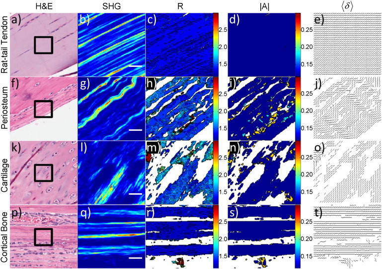
PIPO parameters in tissues with parallel collagen fibril distributions. (Rows a–e) Rat-tail tendon, (rows f–j) periosteum, (rows k–o) tibia cartilage, and (rows p–t) tibia cortical bone, respectively. (a, f, k, and p) White-light images of H&E stained sections. (Black box) 50 × 50 μm² region similar to the SHG images in panels b, g, l, and q. (c, h, m, and r) Corresponding R-ratio images. Coloring corresponds to the R-ratio value and the color-bar ranges from a ratio of 1.2–3.0. (d, i, n, and s) Corresponding |A|-ratio images, where the coloring ranges from 0 to 0.3. (e, j, o, and t) Corresponding fibril orientation images. Each line indicates the direction of the 〈δ〉. (White space) Absence of a ratio. The scale bar is 10 μm.

The H&E and SHG images of the growth-plate region of tibia reveal the distribution of type-II collagen fibers found in hyaline cartilage (Fig. 3, k and l). Though sagittal-cut sections were used, the fibers are not continuously observed throughout the SHG image, suggesting the fibrils are not perfectly oriented in the XZ plane (i.e., the image plane), which results in a higher R-ratio compared to the ${\chi }_{zzz}^{\left(2\right)}/{\chi }_{zxx}^{\left(2\right)}$ of type-II fibrils. The R-ratio image displays uniformity and possesses values (∼1.4–1.6) that fall slightly above those in periosteum and tendon (Fig. 3 m). The |A|-ratio image is similar to the previous two examples, with low asymmetry (∼0–0.1), particularly for areas where strong SHG signal was observed (Fig. 3 n). The fibril orientations were also similar to tendon, showing low variability and a sheetlike distribution (Fig. 3 o). In cortical bone of tibia, H&E and SHG images reveal a parallel organization of collagen fibrils (Fig. 3, p and q). Strips of alternating bright and dark regions in SHG are present with thicknesses of ∼10 μm. The region is close to the insertion of the patellar ligament and likely a mixture of tendon and cortical bone. Cortical bone can be composed of alternating lamellae of collagen fibrils depending on the state of the bone tissue; therefore, the dark regions of SHG could correspond to lamellae with the fibrils oriented orthogonally to the XZ plane. The high R-ratios in the dark regions provide further evidence for orthogonally oriented fibrils (Fig. 3 r). The bright regions in SHG correspond to extremely uniform low R-ratio values in the R-ratio image (Fig. 3 r). The R-ratios (R ∼ 1.2) are the lowest for any collagen measured in all the tissues. This suggests the collagen fibrils lie perfectly in the plane and parallel to the long axis of the tibia. There is no asymmetry present in the cortical bone (Fig. 3 s). The orientation of the collagen fibrils confirms that the preferential direction is along the long axis of the tibia (Fig. 3 t). Additionally, there is no appreciable variability in the orientation of the fibrils for the lamellae imaged. These tissues have low R-ratios (<2), are fairly symmetric (|A| ≈ 0), and the observed collagen fibrils tend to orient in a preferential direction. The R, |A|, and 〈δ〉 images for the parallel fibril organizations may be adequately summarized as having low variability.

By contrast, the tissues containing nonparallel distributions and constant-tilt fibrils (e.g., dermis and cornea (1,4)) showed much greater variability in their PIPO parameters. The H&E and SHG images of dermis display a dramatically different distribution from that of the parallel examples previously given (Fig. 4, a and b). The fibers appear as a woven meshwork (Fig. 4, a and b). The R-ratio values are substantially higher than the previous examples (∼1.6–2.2), with domains of alternating R values (Fig. 4 c). The asymmetry is also moderately higher in certain regions (∼0.2) (Fig. 4 d). However, there is no apparent correlation between the R domains and the |A|-ratio. The fibril orientation image also displays alternating regions of fibril direction (Fig. 4 e). The directions of the fibrils show no observable correspondence with the coloring of the R-ratio image. Cornea reveals alternating lamellae of collagen type-I fibrils from the H&E and SHG images (Fig. 4, f and g). The cross-section of the lamellae appears as fibrils in the SHG image (Fig. 4 g). However, the lamellae are more readily observed in the R-ratio image (Fig. 4 h), where alternating regions of higher and lower R values are present (1.5 compared to 1.8).

Figure 4.

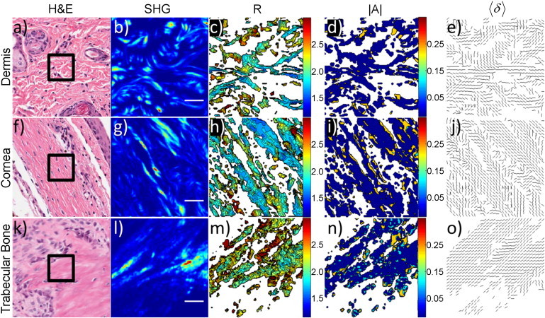
PIPO parameters in tissues with nonparallel collagen fibril distributions. (Rows a–e) Dermis, (rows f–j) cornea, and (rows k–o) vertebrae trabecular bone. (a, f, and k) White-light images of H&E stained sections. (Black box) 50 × 50 μm² region similar to the SHG images in panels b, g, and l. (c, h, and m) Corresponding R-ratio images. (d, i, and n) Corresponding |A|-ratio images. (e, j, and o) Corresponding fibril orientation images. Each line indicates the direction of the 〈δ〉. All coloring is the same as Fig. 3.The scale bar is 10 μm.

The |A|-ratio image possesses higher values (∼0.2) near the boundaries of apparent lamellae compared to the straight fibril examples (Fig. 4 i). The fibril orientation image, like the dermis, shows alternating regions of preferential direction (Fig. 4 j). The domains of preferential direction appear weakly correlated with the R-ratio image, suggesting uniformity within the lamellae.

Trabecular bone in the vertebra displays a woven pattern of threads with a preferential direction in the H&E and SHG images (Fig. 4, k and l). The R-ratio image shows the highest values (∼1.8–2.5) of the tissue samples investigated (Fig. 4 m); however, the variability is lower than that of dermis and cornea. The |A|-ratio image reveals a broader distribution of values (∼0.1–0.2) compared to dermis and cornea (Fig. 4 n). The fibril orientation in trabecular bone is affected by the history of the mechanical stresses on the bone. The collagen fibrils organize into interconnected rods and plates, which form a lattice structure of bone filled with bone marrow (35–37). The fibril orientation image shows fibrils preferentially oriented with low variability along the fibril directions observed in the SHG image (Fig. 4 o).

For a more quantitative comparison of the PIPO parameters of the various tissues, construction of occurrence histograms is informative (Fig. 5). For each tissue, seven-to-ten 50 × 50 μm² regions were investigated and only fitting parameters possessing an adjusted-R² > 0.99 were used (∼10⁴ data points per distribution). Two different shapes of histograms arose: a narrow distribution and a broad skewed distribution. Cortical bone of tibia (R ∼ 1.1–1.5), tail tendon (R ∼ 1.2–1.5), periosteum (R ∼ 1.2–1.8), and growth plate cartilage (R ∼ 1.3–2.2) displayed the former type of distribution, whereas dermis (R ∼ 1.5–2.7), cornea (R ∼ 1.5–2.7), and trabecular bone in vertebrae (R ∼ 1.8–3.0) displayed the latter type of distribution (Fig. 5 a). The shape of the distribution correlates well with the symmetry of the tissue observed in SHG images (i.e., parallel versus nonparallel). Furthermore, the observed spatial organization of collagen in the SHG images corresponds well with scanning electron microscopy (SEM) and transmission electron microscopy studies previously performed on similar tissues (33–38). In addition to the shape of the distribution, the minimum value for R, R_min, corresponds to the ${\chi }_{zzz}^{\left(2\right)}/{\chi }_{zxx}^{\left(2\right)}$ of the fibrils, when the distributions of α and Δδ are narrow and lie in the XZ plane (see Eq. 5).

Figure 5.

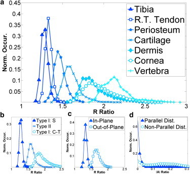
Occurrence histograms of PIPO parameters. (a) Occurrence histograms of the R ratios for tibia cortical bone (triangle), rat tail tendon (box), periosteum (star), tibia cartilage (cross), dermis (diamond), cornea (circle), and vertebrae trabecular bone (plus). (b) Histogram of R ratios for straight type-I fibrils (triangle), type-II fibrils (cross), and constant-tilt type-I fibrils (circle). (c) Histogram of R ratio showing the effect of in-plane (triangle) and out-of-the-plane (circle) fibrils in rat-tail tendon. (d) Histogram of |A| for parallel (triangle) and nonparallel (circle) fibril distributions. Only fits with an adjusted-R² value > 0.99 were used for the construction of the histograms.

Histograms of the different fibril models and types were constructed (Fig. 5 b). The R_min ratios for straight type-I (tendon), type-II (cartilage), and constant-tilt type-I (dermis, cornea) were 1.24 ± 0.03, 1.38 ± 0.05, and 1.58 ± 0.08, respectively. The difference between the R_min of straight and constant-tilt fibril tissue is statistically significant according to the Welch t-test. Using Eq. 1, a constant-tilt angle of ∼19° is calculated, corresponding well with various studies performed on dermis and cornea tissue (1,4). The R_min for trabecular bone in vertebrae was 1.9 ± 0.1. The distribution and minimum are higher than all the other tissue types, likely due to the crossing of fibrils or lamellae in trabecular bone (35–37), which is simply the result of sectioning at an angle to the fibrils or lamellae. The R_min values for straight type-I and type-II are also statistically distinguishable. However, the uncertainty in the α-distribution of the type-II fibrils diminishes the statistical significance. Multiple samples were sectioned along the sagittal axis, with no sample giving perfectly parallel fibrils like those observed for type-I. To demonstrate the effect of a nonzero α-distribution, rat-tail tendon (in-plane) is compared to rat-tail tendon (out-of-plane). From the SHG images (e.g., Fig. 2 c), it is apparent that the tendon fibers lie out-of-the-plane for samples not elongated during fixation. The effect is a shift to higher R-ratios (∼1.35–1.65), corresponding to an average angle to the image plane of 25°. The overall shape of the distribution is not appreciably altered from the shift. However, the width of the distribution widens slightly due to the second derivative of Eq. 5 with respect to α.

To measure the asymmetry of the PIPO plots, the following formula was utilized:

$$a=\langle \left|\frac{I\left(\theta ,\phi \right)-I\left(-\theta ,-\phi \right)}{\raisebox{1ex}{$1$}\!\left/ \!\raisebox{-1ex}{$2$}\right.\left(I\left(\theta ,\phi \right)+I\left(-\theta ,-\phi \right)\right)}\right|\rangle .$$ (8)

where I(θ,φ) is the SHG intensity for the angles θ and φ, which are defined from 0 to π/2 (i.e., upper-left PIPO quadrant). This measures a spread in intensity around an average intensity of the PIPO plots at each pixel. This asymmetry has distributions centered on zero for both parallel (cortical bone in tibia) and nonparallel (dermis and cornea) tissue distributions (see Fig. S1 in the Supporting Material) with the nonparallel fibril distribution having a more pronounced tail than the parallel. Comparing this result to the distribution of the |A|-ratio confirmed its validity for measuring the PIPO plot asymmetry, with the |A|-ratio distributions being more pronounced (Fig. 5 d). The asymmetry is likely influenced by both the collagen distribution and the focusing conditions of the optical setup. Therefore, care should be taken when interpreting the |A|-ratio in terms of the collagen organization. The maximum |A| was larger for the nonparallel fibril distributions than the parallel (∼0.3 compared to ∼0.05). Both |A|-ratio distributions had center peaks on zero; however, the nonparallel fibrils had a secondary peak at ∼0.15–0.2 (Fig. 5 d).

The parameters R, |A|, and 〈δ〉 relate to the underlying structure of the collagen fibrils. A priori, if information is known about the tissue (e.g., hyperpolarizability ratio of the fibrils, parallel symmetry, etc.), then three-dimensional structural information may be inferred from the P-SHG data. As an example, if a parallel distribution (i.e., α and δ are constant in each voxel) is assumed to be comprised of straight fibrils, then R and 〈δ〉 may be used to determine the three-dimensional organization of the collagen fibrils. With the assumption of a single fibril, Eq. 5 can be used to extract the angle α. With the modified spherical coordinates, α and δ, the orientation of the fibrils in the tissue section may be visualized (Fig. 6). In Fig. 6, the scalar color bar indicates the R value for each voxel (included for visual clarity), where the voxel is represented as a cylindrical fibril. The structure visualized is the intervertebral disk in a rat vertebrae section. The outer region of the disk (predominately type-I (2)) reveals alternating stacked lamellae. The blue fibrils orient roughly at an average angle of −20° to the XZ plane, whereas the red fibrils are oriented in the opposite direction, roughly at an average angle of 40° to the XZ plane (Fig. 6 a). This is consistent with the expected structure of intervertebral disk, and similar structures were observed with SEM images of a similar region of the tissue (Fig. 6 b). Because Eq. 5 is an even function, there is degeneracy in α and, therefore, Fig. 6 shows only one possible organization from a larger set of possibilities. Nevertheless, there is value in visualizing the three-dimensional architecture, even if it is only representative and not absolute.

Figure 6.

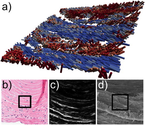
Structural visualization of intervertebral disk. (a) Three-dimensional reconstruction of intervertebral disk in the rat vertebrae section where cylinders represent an average fibril at each pixel. Coloring indicates the R ratio for visual clarity (blue is ∼1.45 and red is ∼1.95). (b) H&E image of a similar region of intervertebral disk. (c) SHG image of the disk. (d) SEM image of a similar region of the disk. (Black boxes) 50 × 50 μm² region.

Discussion

Hierarchical structure of collagen

The popularity of P-SHG microscopy for investigating fibrillar collagen-rich tissue is increasing (18,19), along with the desire to extract as much structural information as possible. Often in the literature, the average R-ratio is interpreted as resulting from the pitch of the collagen triple-helix (24), the type of collagen (26), or the angle of the collagen fibril with respect to the image plane (30,39). Though all are valid, there is a danger in focusing solely on one and neglecting other equally important effects resulting from the hierarchical nature of collagen in tissue. The structure of collagen at every level of organization must be understood to interpret P-SHG data. Useful hierarchical levels for the interpretation of P-SHG data are: fibril organization in biological tissue (e.g., fibers, lamellae), the ultrastructure of individual fibrils (e.g., straight, constant-tilt), and the molecular composition of collagen fibrils (e.g., type-I, type-II). With this framework in mind, interpretation of P-SHG data can be made in a more consistent manner across various tissues.

Fibril organization in biological tissue

A number of different fibril organizations were investigated in this study (e.g., the parallel fibers of rat-tail tendon, the lamellae of cornea, and the woven meshwork of dermis). For parallel distributions, the effect of fibrils orienting out of the image plane was presented for rat-tail tendon (Fig. 5 c), where according to Eq. 5 the out-of-plane fibrils showed an expected increase in R relative to in-plane fibrils (∼1.65 compared to ∼1.35). The high R-ratio for dermis, cornea, and trabecular bone of vertebrae, however, should be interpreted in terms of collagen fibrils oriented nonuniformly. Electron microscopy studies of dermis, cornea, and trabecular bone reveal a woven meshwork of fibrils for dermis, stacked lamellae for cornea, and a porous organization of rods and plates for trabecular bone (33,35–38). This can lead to a nonzero distribution in Δδ and α, depending on the section angle, which leads to a higher R-ratio following Eq. 5. The dependence on the sectioning angle is tissue-dependent. From the occurrence histograms of cortical and trabecular bone (Fig. 5 a), the effect of sectioning and fibril organization is evident. When sectioning is along the axis of the collagen fibrils, the R-ratio is minimized; however, when fibrils grow in a distribution of orientations to the section plane, the R-ratios are appreciably higher (>1.9).

The PIPO occurrence histograms are analogous to a fingerprint for particular regions of tissue, with every region of tissue possessing a unique pattern (Fig. 5 a). Nevertheless, as with fingerprints, there are certain universal attributes accessible from studying the PIPO histograms. One such attribute is the shape of the distribution, which appear to provide insight into the underlying spatial symmetries of the fibril organization. An observed general rule-of-thumb, useful in developing an intuition, is a narrow distribution corresponds to parallel tissue symmetry (i.e., well-aligned fibrils), whereas broad distributions correspond to nonparallel systems (i.e., woven meshwork). A positive correlation between R-ratio values and the distribution widths was also observed, simply the result of the nonlinear nature and curvature (i.e., second derivative with respect to α and Δδ), and of Eq. 5.

R_min ratio and the ultrastructure of fibrils

Another attribute accessible from studying the PIPO histograms is the ${\chi }_{zzz}^{\left(2\right)}/{\chi }_{zxx}^{\left(2\right)}$ ratio of a collagen fibril. Often in the literature, the average R-ratio is quoted for the collagen fibril types; however, this value includes additional information regarding average fibril organization. Thus, a measure of the R_min ratio of a tissue region seems a better indicator of the ${\chi }_{zzz}^{\left(2\right)}/{\chi }_{zxx}^{\left(2\right)}$ ratio of a particular type of collagen fibril, because following Eq. 5 this corresponds to minimal contribution from the spatial organization of the fibrils in the tissue (i.e., α = Δδ = 0). For straight type-I fibrils, where all of the collagen triple-helices are aligned parallel to the fibril axis, the fibril ${\chi }_{zzz}^{\left(2\right)}/{\chi }_{zxx}^{\left(2\right)}$ ratio corresponds to the β_zzz/β_zxx ratio of the type-I collagen triple-helix (28,29). The results, therefore, suggest that the type-I collagen triple-helix has a β_zzz/β_zxx ratio of 1.24 ± 0.03. This value is slightly lower relative to the average values (1.3–1.4) often cited in the literature (14–17,24,25), though it is in reasonable agreement with recent quantum mechanical calculations performed on a GLY-PRO-HYP collagen model (R ∼ 1.4) (28).

Using β_zzz/β_zxx = 1.24 ± 0.03 for type-I collagen and following Eq. 1, the tilt angle of the triple-helices in fibrils of dermis and cornea was ∼19°, which is in excellent agreement with multiple electron microscopy studies (1,4). The angle estimation used an R_min ratio of 1.58 for the constant-tilt fibrils. The expected R_min ratio, assuming a tilt angle of 16–18°, is 1.47–1.54. The higher R_min for the constant-tilt fibrils is likely due to contributions from α and Δδ. This highlights an important point that while the R_min ratio attempts to determine the ${\chi }_{zzz}^{\left(2\right)}/{\chi }_{zxx}^{\left(2\right)}$ of the individual fibrils, there is no guarantee, if the section does not contain any well-aligned fibrils (i.e., parallel and in-plane). The very high R_min ratio, 1.9 ± 0.1, for trabecular bone in vertebrae is also likely due to the packing arrangement of the collagen fibrils in the section and not the internal structure of the individual fibrils. When fibrils in bone are well aligned—as they were for the cortical bone of the tibia sample—an R_min ratio of ∼1.2 was observed.

R_min and collagen type

As with straight type-I, the R_min ratio for type-II fibrils should correspond to the β_zzz/β_zxx ratio of type-II triple-helices. There is evidence that the type-II fibril banding pattern is 67 nm, like for type-I straight fibrils in rat-tail tendon (40). This implies the β_zzz/β_zxx of type-II is 1.38 ± 0.05 compared to 1.24 ± 0.03 for type-I. This is somewhat surprising as the variation in the amino-acid composition between type-I and -II is minimal, equal to the intrachain variation of type-I (2). Nevertheless, these preliminary results suggest a difference. Despite attempts for perfect sectioning, the most reasonable explanation is a nonzero α-distribution. This is evidenced by the observation that the fibrils are not continuously present throughout the 50-μm SHG images as they are for the tail tendon sample (see, for example, Fig. 3). Alternatively, internal cross-linking of type-II has been suggested to be different from type-I (40), which could result in a different R_min ratio. Further investigations must be carried out to elucidate the origin of the discrepancy between type-I and type-II fibrils, irrespective of fibril organization.

The magnitude of the difference between type-I and -II fibrils is substantially smaller than that previously reported by Su et al. (41). The disparity may be explained by a number of factors. To start, different tissues (rat epiphyseal cartilage compared to rat trachea) and different imaging conditions were used (e.g., 800 nm compared to 1030 nm, as well as different numerical apertures). Additionally, from the SHG images of Su et al. the collagen type-II-containing tissues appear nonparallel. Therefore, the substantial differences in R values observed by Su et al. for the different types of collagen are also likely due to the organizational differences of the collagen fibrils within the tissues.

Conclusions

The three polarization parameters extracted from P-SHG microscopy experiments—$R={\chi }_{ZZZ}^{{\left(2\right)}^{\prime }}/{\chi }_{ZXX}^{{\left(2\right)}^{\prime }}$, the second-order susceptibility ratio; |A|, a measure of the fibril distribution asymmetry; and 〈δ〉, the weighted-average fibril orientation—should be understood in terms of the hierarchical organization of collagen, which includes

• 1.collagen type determined by the sequence of amino acids in the triple-helix,
• 2.fibril internal structure mostly affected by the triple-helix tilt angle to the fibril axis, and
• 3.the tissue-specific distribution of fibrils within the three-dimensional volume of each voxel of the image.

Using the hierarchical model, quantifiable differences between straight fibrils (rat-tail tendon) and constant-tilt fibrils (dermis and cornea) are observed, leading to the correct prediction of the triple-helix tilt angle with respect to the fibril axis. The fibril organization is differentiated through occurrence histograms of R and |A|, which distinguishes parallel from nonparallel fibril distributions. Additionally, the histograms provide a measure of R_min, which offers a prediction of the fibril R-ratio. With knowledge of the R-ratio of the fibrils, as well as the 〈δ〉 angles, three-dimensional reconstruction of the distribution of fibril orientations in tissue can be deduced. The three-dimensional fibril distribution of lamellae in intervertebral disk was presented as a demonstration, visualizing correctly the alternating orientations of collagen fibrils within neighboring lamellae. Therefore, the hierarchical model of fibrillar collagen and the measured R, |A|, and 〈δ〉 parameters of the tissue, provide a method for quantifying tissue architecture, when the tissue-specific ${\chi }_{ZZZ}^{\left(2\right)}/{\chi }_{ZXX}^{\left(2\right)}$ ratio of the fibrils (often similar to R_min) is known a priori.

Appendix A: Dependence Of Second-Order Susceptibility Ratios On Collagen Organization

From general tensor rotation theory,

$${\chi }_{IJK}^{{\left(2\right)}^{\prime }}=T_{Ii}{T}_{Jj}{T}_{Kk}{\chi }_{ijk}^{{\left(2\right)}^{\prime }},$$ (A1)

where T_mn is the mn^th element of a rotation matrix and Einstein summation is implied. For rotations, first by δ about the Y axis and then by α about the Z axis, the susceptibility elements may be expressed as

$${\chi }_{ZZZ}^{{\left(2\right)}^{\prime }}=\text{cos}\alpha \text{cos}\delta \left[\left({\chi }_{zzz}^{\left(2\right)}/{\chi }_{zxx}^{\left(2\right)}-3\right){\text{cos}}^2\alpha {\text{cos}}^2\delta +3\right]{\chi }_{zxx}^{\left(2\right)},$$ (A2)

$${\chi }_{ZXX}^{{\left(2\right)}^{\prime }}=\text{cos}\alpha \text{cos}\delta \left[\left({\chi }_{zzz}^{\left(2\right)}/{\chi }_{zxx}^{\left(2\right)}-3\right){\text{cos}}^2\alpha {\text{sin}}^2\delta +1\right]{\chi }_{zxx}^{\left(2\right)},$$ (A3)

$${\chi }_{XXX}^{{\left(2\right)}^{\prime }}=\text{cos}\alpha \text{sin}\delta \left[\left({\chi }_{zzz}^{\left(2\right)}/{\chi }_{zxx}^{\left(2\right)}-3\right){\text{cos}}^2\alpha {\text{sin}}^2\delta +3\right]{\chi }_{zxx}^{\left(2\right)},$$ (A4)

$${\chi }_{XZZ}^{{\left(2\right)}^{\prime }}=\text{cos}\alpha \text{sin}\delta \left[\left({\chi }_{zzz}^{\left(2\right)}/{\chi }_{zxx}^{\left(2\right)}-3\right){\text{cos}}^2\alpha {\text{cos}}^2\delta +1\right]{\chi }_{zxx}^{\left(2\right)},$$ (A5)

where ${\chi }_{zzz}^{\left(2\right)}/{\chi }_{zxx}^{\left(2\right)}$ is for the collagen fibril. Lower-case coordinates, xyz, refer to the fibril system (i.e., fibril axis along the z axis), whereas XYZ refers to the laboratory coordinate system. If there are multiple fibrils present in the voxel, then the ${\chi }_{ZZZ}^{{\left(2\right)}^{\prime }}$ element may be defined as

$$\begin{array}{c}{\chi }_{ZZZ}^{{\left(2\right)}^{\prime }}=\left[\left({\chi }_{zzz}^{\left(2\right)}/{\chi }_{zxx}^{\left(2\right)}-3\right)\left(\sum _i{\omega }_i{\text{cos}}^3{\alpha }_i{\text{cos}}^3{\delta }_i\right)+3\left(\sum _i{\omega }_i\text{cos}{\alpha }_i\text{cos}{\delta }_i\right)\right]{\chi }_{zxx}^{\left(2\right)}\\ =\left[\left({\chi }_{zzz}^{\left(2\right)}/{\chi }_{zxx}^{\left(2\right)}-3\right)\langle {\text{cos}}^3\alpha {\text{cos}}^3\delta \rangle +3\langle \text{cos}\alpha \text{cos}\delta \rangle \right]{\chi }_{zxx}^{\left(2\right)},\end{array}$$ (A6)

where ω_i is the probability associated with the i^th fibril orientation. The elements ${\chi }_{ZXX}^{{\left(2\right)}^{\prime }}$, ${\chi }_{XXX}^{{\left(2\right)}^{\prime }}$, and ${\chi }_{XZZ}^{{\left(2\right)}^{\prime }}$ may be determined for multiple fibrils in a similar manner. The relevant ratios then may be defined as

$$R=\frac{{\chi }_{ZZZ}^{{\left(2\right)}^{\prime }}}{{\chi }_{ZXX}^{{\left(2\right)}^{\prime }}}=\frac{\left(\frac{{\chi }_{zzz}^{\left(2\right)}}{{\chi }_{zxx}^{\left(2\right)}}-3\right)\frac{\langle {\text{cos}}^3\alpha {\text{cos}}^3\delta \rangle }{\langle \text{cos}\alpha \text{cos}\delta \rangle }+3}{\left(\frac{{\chi }_{zzz}^{\left(2\right)}}{{\chi }_{zxx}^{\left(2\right)}}-3\right)\left(\frac{\langle {\text{cos}}^3\alpha \text{cos}\delta \rangle }{\langle \text{cos}\alpha \text{cos}\delta \rangle }-\frac{\langle {\text{cos}}^3\alpha {\text{cos}}^3\delta \rangle }{\langle \text{cos}\alpha \text{cos}\delta \rangle }\right)+1},$$ (A7)

$$A=\frac{{\chi }_{XXX}^{{\left(2\right)}^{\prime }}+{\chi }_{XZZ}^{{\left(2\right)}^{\prime }}}{{\chi }_{ZZZ}^{{\left(2\right)}^{\prime }}+{\chi }_{ZXX}^{{\left(2\right)}^{\prime }}}=\frac{\left(\frac{{\chi }_{zzz}^{\left(2\right)}}{{\chi }_{zxx}^{\left(2\right)}}-3\right)\langle {\text{cos}}^3\alpha \text{sin}\delta \rangle +4\langle \text{cos}\alpha \text{sin}\delta \rangle }{\left(\frac{{\chi }_{zzz}^{\left(2\right)}}{{\chi }_{zxx}^{\left(2\right)}}-3\right)\langle {\text{cos}}^3\alpha \text{cos}\delta \rangle +4\langle \text{cos}\alpha \text{cos}\delta \rangle }.$$ (A8)

The above ratios are valid for any distribution of collagen fibrils. If a constant α is assumed valid, then Eqs. A7 and A8 simplify to

$$R=\frac{{\chi }_{ZZZ}^{{\left(2\right)}^{\prime }}}{{\chi }_{ZXX}^{{\left(2\right)}^{\prime }}}=\frac{\left(\frac{{\chi }_{zzz}^{\left(2\right)}}{{\chi }_{zxx}^{\left(2\right)}}-3\right){\text{cos}}^2\alpha \frac{\langle {\text{cos}}^3\delta \rangle }{\langle \text{cos}\delta \rangle }+3}{\left(\frac{{\chi }_{zzz}^{\left(2\right)}}{{\chi }_{zxx}^{\left(2\right)}}-3\right){\text{cos}}^2\alpha \left(1-\frac{\langle {\text{cos}}^3\delta \rangle }{\langle \text{cos}\delta \rangle }\right)+1},$$ (A9)

$$A=\frac{{\chi }_{XXX}^{{\left(2\right)}^{\prime }}+{\chi }_{XZZ}^{{\left(2\right)}^{\prime }}}{{\chi }_{ZZZ}^{{\left(2\right)}^{\prime }}+{\chi }_{ZXX}^{{\left(2\right)}^{\prime }}}=\frac{\langle \text{sin}\delta \rangle }{\langle \text{cos}\delta \rangle }.$$ (A10)

For PIPO experiments, it is often convenient to change coordinates and replace δ with Δδ = δ − 〈δ〉, where 〈δ〉 is the weighted-average fibril orientation.

Appendix B: PIPO SHG Intensity Derivation

The second-harmonic intensity through an analyzer, oriented at the angle φ from the Z axis, can be expressed as

$$I_{2\omega }\propto {\left|\left[\begin{array}{cc}{\text{sin}}^2\phi & \text{sin}\phi \text{cos}\phi \\ \text{sin}\phi \text{cos}\phi & {\text{cos}}^2\phi \end{array}\right]{\overrightarrow{E}}_{2\omega }\right|}^2=\left|E_i{\left(A^2\right)}_{ij}{E}_j\right|,$$ (B1)

where ${\overrightarrow{E}}_{2\omega }\equiv \overrightarrow{E}$ is the harmonic electric field and A is the Jones matrix of an analyzer defined as

$$A=\tilde{A}=\left[\begin{array}{cc}{\text{sin}}^2\phi & \text{sin}\phi \text{cos}\phi \\ \text{sin}\phi \text{cos}\phi & {\text{cos}}^2\phi \end{array}\right],$$

and where $\tilde{A}$ (${\tilde{A}}_{ji}=A_{ij}$) is the transposed matrix, and obeys the property, A² = A (i.e. it is the projection matrix possessing the eigenvalues 1 and 0). It is easy to verify that

$$A^{\prime }=BA{B}^{-1}=\left[\begin{array}{cc}1& 0\\ 0& 0\end{array}\right],$$

where

$$\begin{array}{l}B=\left[\begin{array}{cc}\text{sin}\phi & \text{cos}\phi \\ -\text{cos}\phi & \text{sin}\phi \end{array}\right],\\ B^{-1}=\tilde{B}=\left[\begin{array}{cc}\text{sin}\phi & -\text{cos}\phi \\ \text{cos}\phi & \text{sin}\phi \end{array}\right].\end{array}$$

In a new basis, defined as E^′ = BE, the harmonic intensity is expressed as

$$I_{2\omega }=\left|E_j^{\prime }{\left(A^{\prime }\right)}_{ij}{E}_j^{\prime }\right|.$$ (B3)

Equation B3 is the general PIPO intensity equation. The SHG electric field is

$${\overrightarrow{E}}_{2\omega }\propto \left[\begin{array}{c}{\chi }_{XXX}^{{\left(2\right)}^{\prime }}{\text{sin}}^2\theta +{\chi }_{XZX}^{{\left(2\right)}^{\prime }}\text{sin}2\theta +{\chi }_{XZZ}^{{\left(2\right)}^{\prime }}{\text{cos}}^2\theta \\ {\chi }_{ZXX}^{{\left(2\right)}^{\prime }}{\text{sin}}^2\theta +{\chi }_{ZZX}^{{\left(2\right)}^{\prime }}\text{sin}2\theta +{\chi }_{ZZZ}^{{\left(2\right)}^{\prime }}{\text{cos}}^2\theta \end{array}\right],$$ (B4)

where ${\chi }_{XXX}^{{\left(2\right)}^{\prime }}=T_{Xi}{T}_{Xj}{T}_{Xk}{\chi }_{ijk}^{\left(2\right)}$ and so on, and the incident electric field is assumed to be a unit vector in the XZ plane with θ being the angle between the incident polarization and the Z axis. Substituting Eq. B4 into Eq. B3 gives the general PIPO SHG intensity equation

$$I_{2\omega }\propto {\left|(\text{sin}\phi \left({\chi }_{XXX}^{{\left(2\right)}^{\prime }}{\text{sin}}^2\theta +{\chi }_{XZX}^{{\left(2\right)}^{\prime }}\text{sin}2\theta +{\chi }_{XZZ}^{{\left(2\right)}^{\prime }}{\text{cos}}^2\theta \right)+\text{cos}\phi \left({\chi }_{ZXX}^{{\left(2\right)}^{\prime }}{\text{sin}}^2\theta +{\chi }_{ZZX}^{{\left(2\right)}^{\prime }}\text{sin}2\theta +{\chi }_{ZZZ}^{{\left(2\right)}^{\prime }}{\text{cos}}^2\theta \right))\right|}^2.$$ (B5)

Of course, Eq. B5 can also be found directly from Eq. B1. For the specific case of C_6ν symmetry, Eq. B5 simplifies to

$$I_{2\omega }\propto {\left[\frac{{\chi }_{ZZZ}^{{\left(2\right)}^{\prime }}}{{\chi }_{ZXX}^{{\left(2\right)}^{\prime }}}\text{cos}\phi {\text{cos}}^2\theta +\frac{{\chi }_{XZX}^{{\left(2\right)}^{\prime }}}{{\chi }_{ZXX}^{{\left(2\right)}^{\prime }}}\text{sin}\phi \text{sin}2\theta +\text{cos}\phi {\text{sin}}^2\theta \right]}^2.$$

The derivation assumes birefringence is negligible, which is reasonably satisfied for thin sections of tissue. If the tissue sample of interest is relatively thick, birefringence must be accounted for.

References

- 1.Wess T.J. Collagen fibril form and function. Adv. Protein Chem. 2005;70:341–374. doi: 10.1016/S0065-3233(05)70010-3. [DOI] [PubMed] [Google Scholar]
- 2.Nimni M.E. Collagen: structure, function, and metabolism in normal and fibrotic tissues. Semin. Arthritis Rheum. 1983;13:1–86. doi: 10.1016/0049-0172(83)90024-0. [DOI] [PubMed] [Google Scholar]
- 3.Nimni M.E. Collagen: its structure and function in normal and pathological connective tissues. Semin. Arthritis Rheum. 1974;4:95–150. doi: 10.1016/0049-0172(74)90001-8. [DOI] [PubMed] [Google Scholar]
- 4.Ottani V., Raspanti M., Ruggeri A. Collagen structure and functional implications. Micron. 2001;32:251–260. doi: 10.1016/s0968-4328(00)00042-1. [DOI] [PubMed] [Google Scholar]
- 5.Rich A., Crick F.H.C. The molecular structure of collagen. J. Mol. Biol. 1961;3:483–506. doi: 10.1016/s0022-2836(61)80016-8. [DOI] [PubMed] [Google Scholar]
- 6.Shoulders M.D., Raines R.T. Collagen structure and stability. Annu. Rev. Biochem. 2009;78:929–958. doi: 10.1146/annurev.biochem.77.032207.120833. [DOI] [PMC free article] [PubMed] [Google Scholar]
- 7.Orgel J.P.R.O., Irving T.C., Wess T.J. Microfibrillar structure of type I collagen in situ. Proc. Natl. Acad. Sci. USA. 2006;103:9001–9005. doi: 10.1073/pnas.0502718103. [DOI] [PMC free article] [PubMed] [Google Scholar]
- 8.Ramshaw J.A.M., Shah N.K., Brodsky B. Gly-X-Y tripeptide frequencies in collagen: a context for host-guest triple-helical peptides. J. Struct. Biol. 1998;122:86–91. doi: 10.1006/jsbi.1998.3977. [DOI] [PubMed] [Google Scholar]
- 9.Orgel J.P.R.O., San Antonio J.D., Antipova O. Molecular and structural mapping of collagen fibril interactions. Connect. Tissue Res. 2011;52:2–17. doi: 10.3109/03008207.2010.511353. [DOI] [PubMed] [Google Scholar]
- 10.Strupler M., Pena A.-M., Schanne-Klein M.C. Second harmonic imaging and scoring of collagen in fibrotic tissues. Opt. Express. 2007;15:4054–4065. doi: 10.1364/oe.15.004054. [DOI] [PubMed] [Google Scholar]
- 11.Pena A.-M., Fabre A., Schanne-Klein M.-C. Three-dimensional investigation and scoring of extracellular matrix remodeling during lung fibrosis using multiphoton microscopy. Microsc. Res. Tech. 2007;70:162–170. doi: 10.1002/jemt.20400. [DOI] [PubMed] [Google Scholar]
- 12.Xu R., Boudreau A., Bissell M.J. Tissue architecture and function: dynamic reciprocity via extra- and intra-cellular matrices. Cancer Metastasis Rev. 2009;28:167–176. doi: 10.1007/s10555-008-9178-z. [DOI] [PMC free article] [PubMed] [Google Scholar]
- 13.Brown E., McKee T., Jain R.K. Dynamic imaging of collagen and its modulation in tumors in vivo using second-harmonic generation. Nat. Med. 2003;9:796–800. doi: 10.1038/nm879. [DOI] [PubMed] [Google Scholar]
- 14.Stoller P., Kim B.-M., Da Silva L.B. Polarization-dependent optical second-harmonic imaging of a rat-tail tendon. J. Biomed. Opt. 2002;7:205–214. doi: 10.1117/1.1431967. [DOI] [PubMed] [Google Scholar]
- 15.Stoller P., Reiser K.M., Rubenchik A.M. Polarization-modulated second harmonic generation in collagen. Biophys. J. 2002;82:3330–3342. doi: 10.1016/S0006-3495(02)75673-7. [DOI] [PMC free article] [PubMed] [Google Scholar]
- 16.Stoller P., Celliers P.M., Rubenchik A.M. Quantitative second-harmonic generation microscopy in collagen. Appl. Opt. 2003;42:5209–5219. doi: 10.1364/ao.42.005209. [DOI] [PubMed] [Google Scholar]
- 17.Freund I., Deutsch M., Sprecher A. Connective tissue polarity. Optical second-harmonic microscopy, crossed-beam summation, and small-angle scattering in rat-tail tendon. Biophys. J. 1986;50:693–712. doi: 10.1016/S0006-3495(86)83510-X. [DOI] [PMC free article] [PubMed] [Google Scholar]
- 18.Brasselet S. Polarization-resolved nonlinear microscopy: application to structural molecular and biological imaging. Adv. Opt. Photon. 2011;3:205–271. [Google Scholar]
- 19.Chen X., Nadiarynkh O., Campagnola P.J. Second harmonic generation microscopy for quantitative analysis of collagen fibrillar structure. Nat. Protoc. 2012;7:654–669. doi: 10.1038/nprot.2012.009. [DOI] [PMC free article] [PubMed] [Google Scholar]
- 20.Squier J., Müller M. High resolution nonlinear microscopy: a review of sources and methods for achieving optimal imaging. Rev. Sci. Instrum. 2001;72:2855–2867. [Google Scholar]
- 21.Zipfel W.R., Williams R.M., Webb W.W. Nonlinear magic: multiphoton microscopy in the biosciences. Nat. Biotechnol. 2003;21:1369–1377. doi: 10.1038/nbt899. [DOI] [PubMed] [Google Scholar]
- 22.Moreaux L., Sandre O., Mertz J. Membrane imaging by second-harmonic generation microscopy. J. Opt. Soc. Am. B. 2000;17:1685–1694. [Google Scholar]
- 23.Boyd R.W. 2nd Ed. Academic Press; New York: 2003. Nonlinear Optics. Ch. 1. [Google Scholar]
- 24.Tiaho F., Recher G., Rouède D. Estimation of helical angles of myosin and collagen by second harmonic generation imaging microscopy. Opt. Express. 2007;15:12286–12295. doi: 10.1364/oe.15.012286. [DOI] [PubMed] [Google Scholar]
- 25.Gusachenko I., Latour G., Schanne-Klein M.-C. Polarization-resolved second harmonic microscopy in anisotropic thick tissues. Opt. Express. 2010;18:19339–19352. doi: 10.1364/OE.18.019339. [DOI] [PubMed] [Google Scholar]
- 26.Chen W.-L., Li T.-H., Dong C.-Y. Second harmonic generation χ tensor microscopy for tissue imaging. Appl. Phys. Lett. 2009;94:183902. [Google Scholar]
- 27.Roth S., Freund I. Second harmonic generation in collagen. J. Chem. Phys. 1979;70:1637–1643. [Google Scholar]
- 28.Tuer A.E., Krouglov S., Barzda V. Nonlinear optical properties of type I collagen fibers studied by polarization dependent second harmonic generation microscopy. J. Phys. Chem. B. 2011;115:12759–12769. doi: 10.1021/jp206308k. [DOI] [PubMed] [Google Scholar]
- 29.Deniset-Besseau A., Duboisset J., Schanne-Klein M.C. Measurement of the second-order hyperpolarizability of the collagen triple helix and determination of its physical origin. J. Phys. Chem. B. 2009;113:13437–13445. doi: 10.1021/jp9046837. [DOI] [PubMed] [Google Scholar]
- 30.Gusachenko I., Tran V., Schanne-Klein M.C. Polarization-resolved second-harmonic generation in tendon upon mechanical stretching. Biophys. J. 2012;102:2220–2229. doi: 10.1016/j.bpj.2012.03.068. [DOI] [PMC free article] [PubMed] [Google Scholar]
- 31.Greenhalgh C., Prent N., Barzda V. Influence of semicrystalline order on the second-harmonic generation efficiency in the anisotropic bands of myocytes. Appl. Opt. 2007;46:1852–1859. doi: 10.1364/ao.46.001852. [DOI] [PubMed] [Google Scholar]
- 32.Major A., Cisek R., Barzda V. Femtosecond Yb:KGd(WO4)2 laser oscillator pumped by a high power fiber-coupled diode laser module. Opt. Express. 2006;14:12163–12168. doi: 10.1364/oe.14.012163. [DOI] [PubMed] [Google Scholar]
- 33.Brown I.A. Scanning electron microscopy of human dermal fibrous tissue. J. Anat. 1972;113:159–168. [PMC free article] [PubMed] [Google Scholar]
- 34.Parry D.A.D., Craig A.S. Quantitative electron microscope observations of the collagen fibrils in rat-tail tendon. Biopolymers. 1977;16:1015–1031. doi: 10.1002/bip.1977.360160506. [DOI] [PubMed] [Google Scholar]
- 35.Jayasinghe J.A.P., Jones S.J., Boyde A. Scanning electron microscopy of human lumbar vertebral trabecular bone surfaces. Virchows Archiv. A Pathol. Anat. 1993;422:25–34. doi: 10.1007/BF01605129. [DOI] [PubMed] [Google Scholar]
- 36.Rubin M.A., Jasiuk I., Apkarian R.P. TEM analysis of the nanostructure of normal and osteoporotic human trabecular bone. Bone. 2003;33:270–282. doi: 10.1016/s8756-3282(03)00194-7. [DOI] [PubMed] [Google Scholar]
- 37.Boyde A., Hordell M.H. Scanning electron microscopy of lamellar bone. Z. Zellforsch. Mikrosk. Anat. 1969;93:213–231. doi: 10.1007/BF00336690. [DOI] [PubMed] [Google Scholar]
- 38.Komai Y., Ushiki T. The three-dimensional organization of collagen fibrils in the human cornea and sclera. Invest. Ophthalmol. Vis. Sci. 1991;32:2244–2258. [PubMed] [Google Scholar]
- 39.Erikson A., Ortegren J., Lindgren M. Quantification of the second-order nonlinear susceptibility of collagen I using a laser scanning microscope. J. Biomed. Opt. 2007;12:044002. doi: 10.1117/1.2772311. [DOI] [PubMed] [Google Scholar]
- 40.Antipova O., Orgel J.P.R.O. In situ D-periodic molecular structure of type II collagen. J. Biol. Chem. 2010;285:7087–7096. doi: 10.1074/jbc.M109.060400. [DOI] [PMC free article] [PubMed] [Google Scholar]
- 41.Su P.-J., Chen W.-L., Dong C.Y. Determination of collagen nanostructure from second-order susceptibility tensor analysis. Biophys. J. 2011;100:2053–2062. doi: 10.1016/j.bpj.2011.02.015. [DOI] [PMC free article] [PubMed] [Google Scholar]
Associated Data
This section collects any data citations, data availability statements, or supplementary materials included in this article.