

Abstract
Aerotaxis, the directional motion of bacteria in gradients of oxygen, was discovered in late 19th century and has since been reported in a variety of bacterial species. Nevertheless, quantitative studies of aerotaxis have been complicated by the lack of tools for generation of stable gradients of oxygen concentration, [O2]. Here we report a series of experiments on aerotaxis of Escherichia coli in a specially built experimental setup consisting of a computer-controlled gas mixer and a two-layer microfluidic device made of polydimethylsiloxane (PDMS). The setup enables generation of a variety of stable linear profiles of [O2] across a long gradient channel, with characteristic [O2] ranging from aerobic to microaerobic conditions. A suspension of E. coli cells is perfused through the gradient channel at a low speed, allowing cells enough time to explore the [O2] gradient, and the distribution of cells across the channel is analyzed near the channel outlet at a throughput of >105 cells per hour. Aerotaxis experiments are performed in [O2] gradients with identical logarithmic slopes and varying mean concentrations, as well as in gradients with identical mean concentrations and varying slopes. Experiments in gradients with [O2] ranging from 0 to ~11.5% indicate that, in contrast to some previous reports, E. coli cells do not congregate at some intermediate level of [O2], but rather prefer the highest accessible [O2]. The presented technology can be applied to studies of aerotaxis of other aerobic and microaerobic bacteria.
INTRODUCTION
Bacterial aerotaxis, directional motion of bacteria in gradients of oxygen concentration (sometimes called oxygen taxis), was discovered 130 years ago 1 and has since then been reported in a variety of bacteria. 2, 3 These bacteria range from an obligate aerobe Bacillus subtilis,2-8 to a facultative anaerobe Escherichia coli,2, 3, 5, 9-14 to a microaerophile Azospirillum brasilense,15-20 to an aerotolerant anaerobe Desulfovibrio vulgaris. 21-23 Nowadays, aerotaxis is often considered as a part of more general energy-sensing behavior2, 18, 24, which enables bacterial cells to find microenvironments with the best growth conditions, including optimal concentrations of nutrients, temperature, and oxygen, and for photosynthetic bacteria, also optimal light intensity. Aerotaxis is considered to be an important mechanism of spatial organization for various bacterial species in stratified microbial mats growing on submerged moist surfaces.2, 25 In addition, some pathogenic bacteria have been shown to be sensitive to [O2] in their environment: Helicobacter pylori are microaerophilic, preferring environments with the oxygen concentration, [O2], of ~5%, 26 and Salmonella typhimurium 4, 9, 11 and Vibrio cholerae27 exhibit full-scale aerotactic behaviors.
Bacterial aerotaxis has been studied with several experimental techniques. In a temporal gradient assay, a bacterial culture in a thin film is exposed to abrupt variations of [O2] by changing the gas mixture surrounding the culture (between O2, N2, and various O2/N2 mixtures), and changes in the swimming behavior of cells are monitored. More frequent tumbling is associated with a change to less favorable [O2] conditions, whereas less frequent tumbling (smooth swimming) is associated with a change to more favorable conditions.4, 17, 28 The temporal assay can be performed rapidly and is useful for testing the aerophilic and aerophobic responses of cells to different [O2], for establishing the approximate range of [O2] preferred by different cells, and for testing the effects of various genetic modifications on aerotaxis.14, 17, 28 However, this technique is not very practical for accurate quantification of the preferred values of [O2] and cannot fully substitute for studying bacterial aerotaxis in spatial gradients of [O2].
In several different spatial aerotaxis techniques, gradients of [O2] are generated in bacterial cultures in capillaries or narrow slits by the combined action of bacterial respiration and diffusion of O2 from an O2-rich gas phase into an O2-deficient culture. 2, 4, 17, 28 Bacterial cells in the capillaries often form distinct bands across the gradient direction, suggesting the existence of preferred values of [O2], which are estimated from the analysis of the diffusion of O2 and distributions of cells in the cultures. 4, 17, 28 Nevertheless, the actual profile of [O2] in the capillary is difficult to evaluate, because it is directly related to the spatial distribution of cells and the rate of O2 consumption per unit volume. The O2 consumption rate is the product of the local density of cells and their average rate of respiration, which by itself is expected to depend on the local value of [O2]. Improved estimates of the range of [O2] preferred by given bacteria can be obtained by varying [O2] in the gas phase and monitoring the resulting changes in the spatial position of the bacterial band17. However, the precision of these estimates is always limited by the incomplete knowledge of the [O2] distribution as well as by the finite width of the bacterial band and variation of [O2] across the band. Direct measurements of [O2] in a capillary with a cell culture were performed with microelectrodes, but their precision was limited by the technique’s sensitivity of ~1%. 17
With a combination of temporal changes of [O2] in thin films and aerotaxis experiments in [O2] gradients in capillaries, the preferred levels of [O2] were evaluated as 3 – 5 μM (0.2 – 0.4%) for A. brasilense17 and ~250 μM (21%) for B. subtilis.4 The preferred level of [O2] for D. vulgaris (aerotolerant anaerobe) was measured with a capillary gradient assay at <0.5 μM (<0.04%). Aerotaxis of E. coli is one of the most extensively studied 2, 3, 5, 9-14, 29, with two key receptor proteins clearly identified: Aer, which is specifically responsible for [O2] sensing (along with other types of energy-sensing), 12, 14 and Tsr, which is also important for chemotaxis in gradients of some soluble factors. 2, 5, 14, 29 Temporal and spatial tests have shown that aerobically cultured E. coli are repelled by both anoxic (pure N2) and hyperoxic (pure O2) conditions, while being attracted to moderate levels of [O2].4, 14, 28 Nevertheless, the exact range of [O2] preferred by E. coli has remained evasive (likely, due to the difficulty of interpreting results of the capillary gradient assays), with some references to unpublished results stating it as 40 - 50 μM 2, 14 (corresponding to an O2 content of 3-4% in the gas phase).
Microfluidic technologies developed in the last decade have been applied by several groups to studies of bacterial chemotaxis in gradients of soluble factors.30 In an early work, Mao et al. fed a suspension of E. coli to an inlet of a long channel, with a gradient of an attractant or a repellant across the channel, and measured the distribution of cells across the channel.31 This approach was conceptually different from previous assays of bacterial chemotaxis. It took advantage of new possibilities provided by microfluidics by enabling the interrogation of a large number of cells in each experiment. This approach also enables the assessment of various parameters of chemotaxis by measuring the distributions of cells across the channel at different distances from the inlet.32 Nevertheless, in chemotaxis experiments with the continuous-flow devices, 31,33 the analysis of results is complicated by gradual variation of the gradient with the distance from the inlet due to diffusion of the attractant (or repellant) across the channel.
Detailed studies of bacterial chemotaxis have been performed in microfluidic devices with microchannels cast in hydrogel.34 In these devices, stable linear and non-linear gradients of chemoattractants are established by molecular diffusion between a source and a sink in the absence of flow in the medium.34-37 One important understanding derived from these experiments 36 as well as from experiments on chemotaxis of eukaryotic cells38-41 is that it is more appropriate to characterize a gradient in terms of fractional rather than absolute change of concentration, C, per unit distance, that is, in terms of a logarithmic slope, d ln(C) / dx, rather than, dC / dx. Several groups have also used high gas permeability of microfluidic devices made of polydimethylsiloxane (PDMS) to generate gradients of [O2] in liquid media42-51 and aerotactic responses of B. subtilis47 and Magnetospirillum magneticum strain AMB-151 in microfluidic gradients of [O2] have been demonstrated.
Here, we built and characterized an experimental setup consisting of a computer-controlled three-channel gas mixer48 and a two-layer microfluidic device made of PDMS generating stable linear profiles of [O2] across a long gradient channel, with [O2] as low as 0.25% (corresponding to microaerobic conditions) in the middle. This setup was used to perform the first quantitative study of bacterial aerotaxis in well-defined gradients of [O2]. As in Ref. 31, the gradient channel was continuously perfused with a suspension of E. coli cells, which were allowed sufficient time to explore the [O2] concentration profile and find their preferred position in it. The distributions of cells across the channel near the channel exit were measured, with data on aerotaxis of ~105 different cells collected within <1 hour. Extensive series of experiments on aerotaxis of E. coli cells were performed in linear gradients of [O2] with identical logarithmic slopes, d ln([O2]) / dx, and varying [O2] in the middle, as well as in [O2] gradients with identical [O2] in the middle but different slopes.
EXPERIMENTAL
Microfluidic device
The microfluidic device we constructed and used in the experiments on E. coli aerotaxis (Fig. 1 and Supplementary Fig. S-1) is made of two layers of PDMS and has two layers of channels. The lower layer of channels, which is adjacent to the cover glass, has channels of two depths, 37 and 150 μm, forming three disconnected networks. The channel network in the middle is used to perfuse a bacterial suspension from the inlet to the outlet through a long rectilinear gradient channel (long channel oriented along the y-axis in the middle in Fig. 1a), which has a width w = 500 μm and a depth of 37 μm. A long serpentine-shaped 37 μm deep channel between the end of the gradient channel and the device outlet (with a 30 μm width and ~110 mm total length) provides hydrodynamic resistance to achieve a mean speed of ~33 μm/s in the gradient channel at a differential pressure of 1 kPa applied between the inlet and outlet. The vent, which is connected to the inlet by a low-resistance 150 μm deep channel, enables rapid flow from the inlet to the gradient channel entrance, when the device is loaded with a bacterial suspension. The vent is blocked during normal operation of the device (aerotaxis assay).
Figure 1.
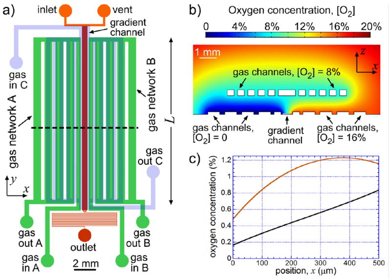
Microfluidic device for experiments on bacterial aerotaxis. (a) Drawing of microchannels in the device. 37 μm and 150 μm deep liquid-filled channels in the lower layer are drawn in red and orange, respectively. 150 μm deep gas channels in the lower layer (in-plane networks A and B) are drawn in green, and 340 μm deep gas channels in the upper layer (out-of-plane network C) are drawn in partially transparent light blue, which is overlaid on the drawing of the lower layer channels. Gas inlets A, B, and C and gas outlets A, B, and C are labeled as gas in A, B, and C and gas out A, B, and C, respectively. (b) Results of a two-dimensional steady-state numerical simulation of the distribution of [O2] (color-coded) in the xz-cross-section of the PDMS chip along the dashed line in (a). The computational domain was 20×5 mm (size of the chip) with an impermeable boundary at the bottom (cover glass) and [O2] = 20.8% at the top and on the sides. Other boundary conditions were [O2] = 0 at the boundaries of the gas channel network A, [O2] = 16% at the boundaries of the gas channel network B, and [O2] = 8% at the boundaries of the gas channel network C. A bottom-central 11×4 mm fragment of the computational domain is shown. (c) [O2] as a function of the position across the gradient channel, x, counted from the left edge from a numerical simulation with [O2]A = 0, [O2]B = 1%, and [O2]C = 0.5% (black curve). Red curve shows results of a simulation for a device without the gas channel network C, with [O2]A = 0 and [O2]B = 1%.
The two other channel networks in the lower layer (Fig. 1a) are mirror-symmetric gas channel networks A and B, which consist of 150 μm deep channels with low flow resistances and are ventilated with different O2/N2 gas mixtures fed to their inlets, gas inlet A (gas in A in Fig. 1a) and gas inlet B (gas in B in Fig. 1a), respectively. The gas mixtures are released to the atmosphere from two outlets, gas outlet A (gas out A) and gas outlet B (gas out B), respectively. The two gas channel networks, which are in the same plane as the liquid-filled channels (in-plane gas channel networks), create a gradient of oxygen concentration, [O2], across the liquid-filled gradient channel. The upper channel layer has a single gas channel network, network C, consisting of 340 μm deep channels, which are ventilated with a third O2/N2 mixture fed to gas inlet C, (gas in C in Fig. 1a), and released from gas outlet C (gas out C). This out-of-plane gas channel network is essential for generation of near-linear profiles of [O2] in the gradient channel, as explained below. The microfluidic chip is assembled out of two layers of PDMS (Sylgard 184 by Dow Corning) with thicknesses of 1.1 and ~4 mm for the lower and upper layer, respectively, which are cast using two separate master molds. Each master mold is a silicon wafer with a relief of SU8 UV-curable epoxy on it and is fabricated using standard photolithography and rapid prototyping protocols. The two PDMS layers are aligned with respect to each other under a microscope and bonded together using oxygen plasma treatment. The two-layer chip is bonded to a #1.5 cover glass by overnight backing in an 80 °C oven.
The goal of the aerotaxis assays was to obtain steady-state distributions of motile bacteria in various linear profiles of [O2] applied across the gradient channel (along the x-axis; Fig. 1). In a widely used biased random walk (one-dimensional diffusion with drift) model of chemotaxis52, 53, when a gradient of a chemoattractant is applied along the x-axis, cells move randomly with an effective diffusivity D and have a chemotaxis-driven velocity (bias), v, along the x-axis. The steady state distribution of cells is given by equation C(x) = C0 exp(vx/D), where C(x) is the concentration of cells at location x and C0 is their concentration at x = 0. The equation indicates that at given D and v, the difference in the concentrations of cells along the gradient field is an exponentially increasing function of the x-axis extension of the field. For the proposed experimental system, this extension is limited by the width of the gradient channel, w. Therefore, to clearly observe the effects of chemotactic or aerotactic migration, it is preferable to have large w. On the other hand, to reach a steady state distribution starting from a near-uniform distribution (as at the gradient channel inlet) in a gradient stretching over a distance w, cells need time, Δt, on the order their diffusion time across the gradient, w2/(2D).
The time available to cells in the microfluidic aerotaxis assay is their residence time in the gradient channel, Δt = Le/vf, where Le is the effective length of the gradient channel and vf is the mean flow velocity in it. Therefore, Δt = w2/(2D) implies vf ≈ 2DLe/w2 for the maximal allowed flow velocity. So, at given Le, large w necessitates low vf, leading to a low experimental throughput. The throughput can be defined as the number of cells interrogated per unit time and is thus proportional to the concentration of cells, the depth of optical field of the video-microscopy system, the width of the gradient channel, and the flow velocity in the channel. In addition, large w leads to a quadratically long transition period (characteristic time Δt = w2/D), after the gradient is modified.
We chose w = 500 μm (similar to the width used before in experiments on E. coli chemotaxis)36, leading to an equilibration time of Δt = w2/(2D) ≈ 312 s at D = 400 μm2/s, which was previously reported for random motion of motile E. coli.52 The effective length of the gradient channel was relatively large at Le = 13.3 mm, so the equation v = 2DL/w2 suggested a flow speed of 43 μm/s. The value of Le is defined as the y-axis extension of the segment of the gradient channel where the [O2] profile can be considered constant. It is somewhat smaller than the length L = 15.7 mm from the most upstream to the most downstream point where the gradient channel is surrounded by the gas channels (see below). The relatively large depth of the gradient channel, 37 μm, leads to low hydrodynamic shear (~5 s-1 at vf = 33 μm/s) and also makes sure that occasional defects in the channel roof (as well as cells and debris stuck to the roof and the floor of the channel) are sufficiently far from the channel mid-plane. Therefore, when cells are imaged at the mid-plane, these defects are out of focus and do not complicate the automated detection of cells. On the other hand, the depth is small enough to allow for rapid establishment of a stable [O2] profile across the gradient channel (see below) and for the supply of [O2] through the porous PDMS chip to be sufficient to prevent bacterial respiration from altering the [O2] profile (see Discussion).
There had been two general configurations of microfluidic devices made of PDMS, in which the oxygen content of liquid-filled channels was set by the flow of O2-containing gas mixtures through nearby gas channels. In most devices, the liquid-filled and gas channels were in different layers42, 46-50, 54, 55 (usually, gas channels above liquid-filled channels, as in the device in Fig. 1) that allowed for a lot of flexibility and enabled generation of a variety of [O2] profiles. However, we did not consider this configuration optimal for the intended aerotaxis experiments, because the [O2] profile in the liquid-filled gradient channel would depend on the thickness of the PDMS layer separating it from the gas channels and on the exact alignment of the gas channels with respect to the gradient channel. Indeed, the aerotaxis experiment required a well-defined profile of [O2] across the 500 μm width of the gradient channel that would remain unchanged along its 15.7 mm extension in the y-direction (Fig. 1a). To this end, an array of gas channels oriented along the y-axis (in the upper layer of PDMS) with different [O2] in them would have to be aligned parallel to the gradient channel (in the lower layer of PDMS) with a precision of alignment on the order of 10 μm over 15 mm, a condition difficult to meet. Furthermore, numerical simulations with an array of 150×150 μm gas channels in an upper layer (as in Ref. 48) indicated that in order to obtain a linear profile of [O2] in a 500 μm wide liquid-filled channel with a concentration ratio of ~5 between the channel edges (cf. Fig. 1c), the gas channels would have to be <200 μm above the gradient channels. This relatively small thickness of the PDMS layer above the gradient channel would likely make the gradient channel depth sensitive to the pressure in it and in the gas channels. In addition, the brightfield microscopy of cells in the gradient channel would likely be complicated by the scattering of light from the gas channel walls.
In other devices51, 56, the liquid-filled and gas channels were in the same layer that allowed reaching [O2] as low as 0.3% in the liquid-filled channels. However, our numerical simulations indicated that with this configuration, it would be very difficult to achieve linear gradients of [O2] across a 500 μm wide gradient channel with [O2] in the middle of 1% (cf. red curve in Fig. 1c) or smaller, as was intended for the present study. Therefore, we used a “hybrid” two-layer design, with gas channels both in the same layer as the gradient channel (in-plane gas channels) and in a layer above it (Fig. 1a,b). In this design, the [O2] profile across the gradient channel is primarily defined by [O2] in the mirror-symmetric in-plane gas channel networks A and B on the two sides of the gradient channel. Specifically, the two marginal in-plane gas channels, which are closest to the gradient channel on either side (both 150 μm deep and 400 μm wide) and are 700 μm away from each other, set the boundary conditions of [O2] in the xy-plane of the gradient channel. Importantly, the alignment of the gas channel networks A and B with respect to the gradient channel is made at the stage of lithographic fabrication of a master mold, where it is easy to achieve a practically parallel orientation of the relief features for the gas channels and the gradient channel. The out-of-plane gas channels, forming the gas channel network C, which are ~340 μm deep and at a distance hg ≈ 1.1 mm above the cover glass, are always ventilated with an O2/N2 mixture with [O2] equal to the arithmetic average between the values of [O2] in the networks A and B. The role of the out-of-plane gas channels is to actively shield the gradient channel from the atmospheric air (which has [O2] = 20.8%), facilitating the establishment of linear [O2] profiles with low [O2] in the middle in the gradient channel. (As we did in our previous publications, here and in what follows we report [O2] in percents, corresponding to the molar fraction of O2 in the gas mixture.)
Numerical simulations, in which the microfluidic device was represented by a 20×5 mm two-dimensional domain in the xz-plane with an impermeable boundary at the bottom (cover glass) and [O2] = 20.8% on the sides and at the top (Fig. 1b), indicated that the shielding by the gas network C was very efficient. With pure N2 in all gas channels ([O2] = 0; not shown), [O2] in the gradient channel was <5·10-5 %, equivalent to a medium at equilibrium with an O2/N2 mixture with 0.5 ppm [O2] by molar content, which would be practically zero even for anaerobic bacteria. An [O2] profile in the gradient channel obtained from a simulation with [O2] = 0 and 1% in the gas channel networks A and B, respectively, and [O2] = 0.5% in the network C is shown in Fig. 1c (black curve). Due to the good shielding from the atmospheric air, the profile is symmetric with respect to the middle of the channel (x = 250 μm), with [O2] equal to 0.500% at x = 250 μm. In a region of x from 50 to 450 μm (>50 μm away from the side walls), where the cross-channel distribution of E. coli was measured in the aerotaxis assays (see below), the oxygen gradient, d[O2] / dx, had a mean value of 1.31·10-3 % per μm. Importantly, the standard deviation of d[O2] / dx in the 50μm < x < 450μm internal region was 6.0·10-5 % per μm, which was <0.05 of the mean gradient, indicating that [O2] profile was nearly linear. On the other hand, a simulation without the out-of-plane gas channel layer, showed a greatly distorted [O2] profile (red curve in Fig. 1c), which would be clearly unsuitable for aerotaxis assays.
Nearly constant value of d[O2] / dx in the gradient channel (Fig. 1c) implies that the logarithmic gradient defined as varies nearly 5-fold from a maximum at x = 0 (where [O2] = 0.16%) to a minimum at x = 500 μm (where [O2] = 0.84%). However, the [O2] profile in the gradient channel can still be characterized by a representative logarithmic gradient, which is calculated as the concentration difference across the channel, Δ[O2] = [O2](w) − [O2](0), divided by the concentration in the middle of the channel, [O2]mid, and by w, Δ[O2] /(w·[O2]mid). The value of the logarithmic gradient is 0.0027 μm-1 and it remains unchanged, when [O2] fed to gas inlet B, [O2]B, varies, as long as [O2] fed to gas inlet A, [O2]A, remains zero and [O2] fed to gas inlet C, [O2]C, is 0.5·[O2]B, because Δ[O2] and [O2]mid change proportionally. In fact, the logarithmic gradient of 0.0027 μm-1 obtained with [O2]A = 0 is the highest value for linear [O2] profiles achievable with the device in Fig. 1a. The logarithmic gradient decreases, when [O2]A is made non-zero.
A simulation with hg reduced to 0.7 mm produced an [O2] profile nearly identical to that with hg = 1.1 mm (with the root-mean-square, rms, of the local differences in [O2] between the two profiles at 1/250 of [O2]mid). Therefore, the [O2] profile in the gradient channel had little sensitivity to the thickness of PDMS between the two channel layers. The lateral displacement of the out-of-plane gas channels by as much as 500 μm along the x-axis resulted in an even smaller rms of local differences of [O2], indicating that the sensitivity of the [O2] profile in the gradient channel to the alignment of the out-of-plane gas channels was very little as well. Finally, due to the large width of the central out-of-plane gas channel (1 mm vs. 0.5 mm for the gradient channel width) and its large z-axis distance from the gradient channel, the scattering of light from the walls of the out-of-plane gas channels had nearly no effect on the brightfield micrographs of bacteria in the gradient channel.
In addition to the steady-state simulations discussed in the preceding paragraph, we also performed a dynamic simulation to establish the time required for [O2] in a solution flowing through the gradient channel to reach the steady-state [O2] profile (such as shown in Fig. 1c). With a diffusion coefficient of O2 in PDMS of 3400 μm2/s 57 and ~6-times lower solubility of O2 in water as compared with PDMS, the characteristic equilibration time was found to be τ ≈ 0.44 sec. This value of τ implied that for an [O2] = 0.25% steady state value ([O2]mid in a 0 to 0.5% gradient field, which was the lowest [O2]mid in our experiments; see below), [O2] would change from the initial 20.8% to 0.26% (which is within 1/25th of the steady state value) within time teq = τ ln[(21 − 0.25)/(0.26 − 0.25)] ≈ 3.5 sec. For a mean flow velocity of vf = 33 μm/s, as in our experiments (see below), this time was equivalent to an ~120 μm distance along the gradient channel, which was small compared to the 15.7 mm length of the channel. We also performed a three-dimensional simulation with a simplified configuration of the gas channels to account for the diffusion of O2 through the bulk of the PDMS chip near the entrance and exit of the gradient channel along the y-axis from regions not enclosed by the gas channel network. The simulation showed that at [O2] = 0.25% in all gas channels, [O2] in the gradient channel reaches 0.26% at a distance of 1.2 mm from the most upstream point, where the gradient channel is enclosed by the gas channel networks. Therefore, the effective length of the gradient channel, Le, was ~13.3 mm, 2.4 mm smaller than the apparent length L = 15.7 mm, (Fig. 1a).
Gas supply
The mixtures of O2 and N2 fed to the gas inlets A, B, and C were prepared using a modified version of the computer-controlled multichannel gas mixer (Supplementary Fig. S-1c) described in our previous publication48. The mixer has three independent channels, each consisting of a miniature, fast-action 3-way solenoid valve with a small inside volume (LHDA 1223111H by The Lee Company), a low-volume fluidic resistor connected to the common port of the valve, and a segment of tubing with a relatively large diameter (0.25 in.) and length (150 mm). This tubing segment is positioned downstream from the fluidic resistor and serves as a diffusive mixer for two gases intermittently emerging from the common port of the solenoid valve.48 Each channel of the gas mixer is connected to a gas inlet of the microfluidic device through polyethylene tubing with a 0.5 mm inner diameter (Supplementary Fig. S-1b). The fluidic resistors are ~20 mm long segments of a 150 μm inner diameter fused silica capillary (TSP150375 by Polymicro Technologies) with a laminar flow resistance greater than the resistance of the gas channel networks A and B (and >10 times greater than the resistance of the gas channel network C).
The normally open port of the solenoid valve is connected to a source of high purity N2 (>99.999% by Airgas) pressurized at 5 psi (34.5 kPa), and the normally closed port of the valve is connected to either air or a 2.5%/97.5% O2/N2 mixture (Supplementary Fig. S-1c), which are always at the same pressure as N2. The pressures are set by two sensitive regulators (Bellofram Type 10 with a 2-25 psi pressure range) and measured with a single high-resolution electronic gauge (Heise test gauge with an accuracy of 0.015 psi). Each of the three solenoid valves is switched on and off with the same period of 2 sec using a home-made driver, a National Instruments PCI-6503 card, and a code in MatLab. The ON time (and the duty cycle) of a valve is calculated to achieve the desired proportion of O2 in the O2/N2 mixture emerging from the common port of the valve, using the known values of viscosities of N2, air, and the 2.5%/97.5% O2/N2 mixture (1.747×10⁻⁵, 1.837×10⁻⁵, and 1.758×10⁻⁵ Pa·s, respectively, at 20 °C). 48 The 2.5%/97.5% O2/N2 mixture was used in experiments, where gas mixtures fed to all gas channel networks had [O2] < 2.5%; air was used in all other experiments.
All parts connecting between the N2 cylinder, N2 pressure regulator, solenoid valves, and the gas inlets of the microfluidic device are made of materials with low gas permeability: hard plastics (acrylic, polypropylene, and polyethylene for the 0.5 mm tubing), metals, and black rubber tubing (Viton™) (Supplementary Fig. S-1c). The use of such materials prevents contamination of N2 with the atmospheric O2 on the way from the N2 cylinder to the device and potentially allows reaching very low [O2] inside the device. The volumetric flow rate, Q, through the gas networks A and B was measured at 0.36 mL/sec, and Q through gas network C was measured at 0.57 mL/sec. We performed a numerical simulation of the diffusion of O2 through the PDMS chip (cf. Fig. 1b, c) with [O2] = 0, 1%, and 0.5% fed to the gas inlets A, B, and C, respectively, to evaluate the total diffusive flux of O2 through the walls of the in-plane gas channel with [O2] = 0, which is closest to the gradient channel. The simulation indicated that at Q = 0.36 mL/sec, the O2 diffusion would increase the mean value of [O2] in that gas channel from zero to 1.2×10⁻⁴ % (equivalent to 1.2 ppm of O2), suggesting that the flow of gas through the channel was sufficiently fast to prevent O2 contamination (or change in [O2] in general) due to diffusion through the chip. In another simulation, [O2] was set to 0 in all three gas channel networks, and the cumulative diffusive flux of O2 into the channels of the gas network C was calculated. At a N2 flow rate Q = 0.57 mL/sec, the calculated diffusive flux would increase [O2] in the network C from 0 to 0.0042% or 42 ppm. This simulation thus indicated that the proposed two-layer geometry of the PDMS chip with the active shielding from atmospheric O2 can potentially be used to create near-anaerobic conditions in a large area of liquid-filled channels at the cover glass.
Measurements of oxygen concentration
As in many previous works45, 48, 55, profiles of [O2] in the gradient channel were measured using a solution of O2-sensitive fluorescent dye, ruthenium tris(2,20-dipyridyl) dichloride hexahydrate (RTDP; obtained from Sigma). The intensity of fluorescence of RTDP, I, is related to its fluorescence intensity at [O2] = 0 (pure N2 in all gas channels), I0, through the Stern-Volmer equation, I0/I = 1 + Kq [O2], where Kq is a quenching constant. The value of Kq is calculated from measurements of fluorescence intensity, Iair, when all gas channels are ventilated with air ([O2] = 20.8%) as Kq = (I0/Iair − 1)/20.8%. Therefore, once the values of I0 and Kq are found, [O2] in a given location in the gradient channel can be evaluated by measuring the value of I in this location as
| (1) |
(some representative fluorescence micrographs of the gradient channel with an RTDP solution are shown in Supplementary Fig. S-2).
Unlike in most previous works on controlling [O2] in microfluidic devices, when high resolution in [O2] was required, RTDP was dissolved in a 66% solution of ethanol in water (by mass) rather than in water. Solubility of O2 in this ethanol solution is almost 3 times greater than in water, thus enhancing its quenching effect at a given percent concentration, increasing the value of Kq, and leading to a greater change in I per 1% of [O2] and greater measurement sensitivity. The fluorescence illumination was derived form a high-luminosity blue LED (with a 455nm center wavelength) connected to a stabilized DC power supply, with the illumination intensity varying by <0.1% in a 20 min period. 55 Fluorescence and brightfield microscopy were performed on an inverted microscope (Nikon TE300) with a 20×/0.45 Plan Fluor Ph1 objective, 0.6× video relay lens and a 2/3” digital CCD camera (Basler A102f). The field of view of the video microscopy setup was ~700 μm wide, covering the entire 500 μm wide gradient channel as well as most of the PDMS partitions between the gradient channel and the flanking in-plane gas channels.
Bacterial culture
Aliquots of a single E. Coli cell culture (strain RP437 58 obtained from Prof. J.S. Parkinson) were prepared and frozen at -79.0 °C. Aliquots were grown overnight in TB (Tryptone broth, with 10 g Tryptone from Becton and Dickinson and 5 g NaCl added to 1 L of water and brought to pH = 7 with NaOH) and then resuspended in fresh TB for ~4 hours at a temperature of 31 °C and shaken at 275 rpm until an OD600 of 0.51±0.03 was reached. Cells were spun down and washed with 1x phosphate buffered saline (PBS) solution (140 mM NaCl, 2.7 mM KCl, 10 mM Na2HPO4, and 2 mM KH2PO4) and then spun down again in a 1.5 mL Eppendorf tube and diluted 2:1 in a motility buffer containing 0.1 mM EDTA and 10 mM lactic acid, with pH adjusted by addition of NaOH and the 1x PBS buffer to a final value of ~6.5. The Eppendorf tube with the cell suspension was connected to the microfluidic device through a line of PTFE tubing using a specially made PDMS plug with two small holes in it (Supplementary Fig. S-1). The PTFE tubing was inserted into one of the holes, and the plug was inserted into the Eppendorf tube, such that the end of the PTFE tubing was several millimeters above the bottom of the tube, forming a siphon.56 (The other hole in the plug vented the tube to the atmosphere). A similar Eppendorf tube filled with PBS was connected to the outlet, with the level of the buffer set ~100 mm below the level of the cell suspension, creating an ~1 kPa differential pressure between the inlet and outlet (Supplementary Fig. S-1). Before an aerotaxis assay, the device was filled with a 1% solution of bovine serum albumin (BSA) in PBS for ~30 min to prevent cells from sticking to the glass surface; the BSA solution was subsequently replaced with PBS.
RESULTS
Measurements of oxygen concentration profiles in the gradient channel
The measurements of [O2] were performed using a 167 ppm solution of RTDP in 66% ethanol in water. The solution was perfused through the gradient channel by applying a 1 kPa differential pressure between the inlet and outlet. To evaluate the quenching constant, Kq, [O2] was first set to 0 (pure N2 in all three gas channel networks) and then to 20.8% (pure air in all gas channel networks). The profiles of fluorescence across the gradient channel were measured at these two [O2] settings (with an ~10 min interval allowed for equilibration). In each case, the fluorescence background was accounted for by fitting a second-order polynomial along the x-axis (across the gradient channel) to the pixel values of the images of the PDMS partitions between the gradient channel and the gas channels flanking it (corresponding to ~100 μm on each side with no fluorescent dye; Fig. 1a,b). After the background polynomials were subtracted from the pixel values of the images of the gradient channel, the resulting ratio of the local RTDP fluorescence intensities, I0/Iair, had a practically flat profile across the gradient channel at 50μm < x < 450μm (not shown) with a mean value of ~2.28, corresponding to Kq ≈ 6.15. (The I0 and Iair profiles were both strongly perturbed near the gradient channel walls, and fluorescence in these regions was not analyzed). This value of Kq was a factor of ~2.7 greater than Kq ≈ 2.25 for solutions of RTDP in water.48, 55 The eq. 1 connecting local values of [O2] in the gradient channel with the local values of I0 and I thus became
| (2) |
When the profiles of fluorescence with [O2] = 0 and [O2] = 20.8% in all gas channel were taken repeatedly, we noticed drift in both I0 and Iair that was as much as 1/12 (in relative units) within a day and might have been due to evaporation of ethanol from the solution. When [O2] is near zero, its value calculated from Eq. 2 is very sensitive to the exact value of I0. Therefore, after performing the gradient measurements described in the next paragraph, we reevaluated the I0 profile and used interpolations in time to estimate the values of I0 at the time points when the profiles of I were measured. On the other hand, the ratio I0/Iair fluctuated much less than I0 and the effect of its fluctuations upon the calculated value of [O2] was much smaller. Therefore, a constant ratio I0/Iair = 2.28 (as in eq. 2) was used for all calculations.
We used the intensity of fluorescence of RTDP to measure [O2] profiles in the gradient channel at 6 sets of conditions, which according to our numerical simulation, were expected to result in linear profiles of [O2] with the same logarithmic slope Δ[O2]/(w·[O2]mid) ≈ 0.0027 μm-1 and with the mean absolute slopes, Δ[O2]/w, different by factors of 2. In all cases we had [O2]A = 0 and [O2]C = 0.5[O2]B, while [O2]B was set at 0.5, 1, 2, 4, 8, and 16%. In each case, the intensity of light in a fluorescence micrograph was measured across the gradient channel, and the background was evaluated (using the procedure described in the previous paragraph) and subtracted from the light intensity, providing the local values of the RTDP fluorescence intensity, I. The values of [O2] vs. the position across the channel, x, were calculated using eq. 2 at different [O2]B and plotted in a 400 μm wide internal region, 50μm < x < 450μm (Fig. 2a,b). The [O2] profiles at [O2]B = 4, 8, and 16% (Fig. 2a) are all close to straight lines and are nearly symmetric with respect to the middle of the channel, x = 250μm. The [O2] profiles at [O2]B = 0.5, 1, and 2% (Fig. 2b) are substantially more noisy, because the fluorescence ratio I0/I varies across gradient channel by only 0.02 – 0.08, but are also well fitted by straight lines. The values of [O2] at x = 250μm, [O2]mid, in Fig. 2b are systematically higher by ~0.15% than [O2] expected from the numerical simulations. It is likely due to ~0.01 relative drift in I0, which is unaccounted for. Importantly, the slopes of the linear fits to the experimental plots of [O2] vs. x (which have little sensitivity to the drift in I0) are all very close to the numerical predictions (inset in Fig. 2b) and vary by factors very close to 2, as [O2]B is varied by a factor of 2 from 0.5% to 16%.
Figure 2.
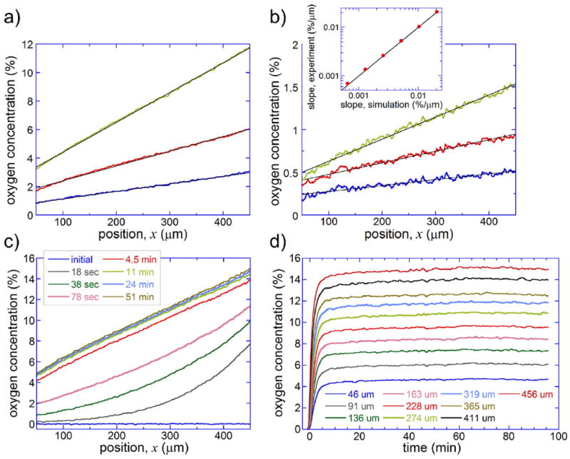
Profiles of [O2] across the gradient channel evaluated from measurements of RTDP fluorescence intensity. (a) [O2] as a function of position, x, across the gradient channel for [O2]B = 4% (blue curve), 8% (red curve), and 16% (green curve). In all cases, [O2]A = 0 and [O2]C = 0.5[O2]B. Black lines are linear fits. (b) [O2] as a function of x for [O2]B = 0.5% (blue curve), 1% (red curve), and 2% (green curve). [O2]A = 0 and [O2]C = 0.5[O2]B in all cases. Black lines are linear fits. Inset: slopes of the linear fits to the experimental curves vs. slopes of linear fits to the results of numerical simulations at the same [O2] settings (red circles). Black line corresponds to identical experimental and numerically calculated slopes. (c) Profiles of [O2] vs. x at different time intervals (as stated in the legend), after [O2]A, [O2]B, and [O2]C have been abruptly switched from their initial value of 0 (pure N2 in all gas channels) to 0, 20.8, and 10.4%, respectively. (d) [O2] as a function of time for different selected positions, x, as stated in the legend (with um standing for μm), after [O2]A, [O2]B, and [O2]C have been switched from 0 to 0, 20.8, and 10.4%, respectively.
To measure the time it takes an [O2] profile in the gradient channel to establish, after [O2]A, [O2]B, and [O2]C are changed, we initially set [O2]A, [O2]B, and [O2]C to zero (pure N2 in all gas channels), then abruptly switched [O2]B to 20.8% (air) and [O2]C to 10.4% (0.5[O2]B), and monitored [O2] vs. x in the gradient channel over time. Because of a relatively large variation of [O2] across the gradient channel in this test (from 3.3 to 17.5%), we used water (rather than 66% ethanol) as the solvent for RTDP, thus reducing the drift in I0 at expense of lower sensitivity of I to [O2] (see Supplementary Fig. S-2). The results of the measurements indicated that the transition to a new [O2] profile was ~9/10 complete within ~4 min (Fig. 2c and d). (The version of the device used in this test had hg = 1.4 mm, and the transition time in the devices with hg = 1.1 mm used in the aerotaxis assays described below was expected to be ~1.6 times shorter.) After the transition, the [O2] profile remained practically steady during the measurement time of ~1.5 hour (Fig. 2c and d). The small variations of [O2] that were recorded during this time could have been due to a combination of a slow drift in the optical system and fluctuations of temperature in the room (modifying the water solubility of O2 by ~0.02 per °C and changing the actual amount of O2 contained in the solution at a given percentage of O2 in the gas phase).
Measurements of distributions of E. coli in the gradient channel
The aerotaxis of E. coli in the linear profiles of [O2] in the gradient channel was quantified by measuring the distributions of E. coli cells along the x-axis (across the channel) at ~1 mm from the channel extit. E. coli suspension was perfused at ~50 μm/s maximal flow velocity (as measured by tracking fluorescent beads at the gradient channel mid-plane), corresponding to ~33 μm/s mean flow velocity at 50μm < x < 450μm and to >400 sec cell residence time in the 13.7 mm long segment of the gradient channel with a constant linear profile of [O2]. Every 10 sec, two brightfield micrographs (Fig. 3a) of a ~500 μm long (y-axis extension) segment of the gradient channel near the mid-plane (~18 μm above the cover glass) were taken with ~0.1 sec interval. The second of the two micrographs was digitally subtracted from the first one to obtain an image revealing moving objects (Supplementary Fig. S-3).
Figure 3.
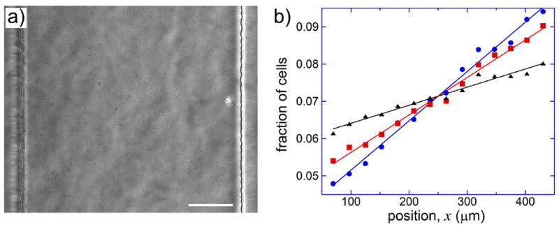
Distributions of E. coli cells in the gradient channel of the microfluidic device. (a) A brightfield micrograph of the gradient channel with E. coli cells taken at [O2]A = 0, [O2]B = 1%, and [O2]C = 0.5% using a 20×/0.75 objective lens. The lens did not have a phase ring, and to enhance the contrast, the microfluidic device was illuminated with a narrow beam directed at an angle to the vertical, resulting in visible short-range non-uniformity of illumination. Scale bar is 100 μm. (b) Fraction of E. coli cells in various ~30 μm wide segments of the gradient channel (x-axis extension) as a function of the position of the segment center, x, at [O2]B = 1% (blue circles), 4% (red squares), and 16% (black triangles). Each set of data points is fitted by a color-matching straight line. For all data sets [O2]A = 0 and [O2]C = 0.5[O2]B. The data was collected on the same day within several hours. The total number of interrogated cells was 0.6·105, 1.2·105, and 1.8·105 for [O2]B of 1%, 4%, and 16% respectively.
The images resulting from the micrograph subtraction were analyzed in a batch mode with a home-made Matlab code that recognized cells and recorded their positions along the x-axis. The parameters of the cell recognition code were optimized by running it on a series of representative images and verifying the results against the assessment of an operator (Supplementary Fig. S-3). The internal region of the gradient channel, 50μm < x < 450μm, was divided into 14 equal segments (bins) and the number of cells in each segment was counted at each time point. The total number of cells in the field of view was typically ~600 (Fig. 3a and Supplementary Fig. S-3). The data at each set of [O2] was taken for 15 – 30 min, bringing the cumulative number of interrogated cells to 0.5 – 1·105. Importantly, with the 10 sec interval between the consecutive images, the 500 μm y-axis extension of the field of view, and the 33 μm/s mean flow velocity, ~66% of the interrogated cells were counted only once. Therefore, the collected entries to the cell distribution bins were mostly statistically independent and represented different individual cells at the end of their 400 sec passage through the gradient channel.
Representative distributions of E. coli cells along the x-axis (Fig. 3b) at [O2]B = 1%, 4%, and 16% and [O2]A = 0 all show clear bias of cell positions towards higher [O2]. The distributions also indicate that the bias decreases at greater [O2]B. The biased random walk model predicts exponential distribution of cells. However, given that in all cases the fractions of cells, n(x), varied between different channel segments by factors ≤2, we found it appropriate to use linear fits, n(x) = ax + b. The strength of aerotaxis at a given set of conditions can be quantified by the slope of the linear fit, a. Given the normalization of the distribution, and , the slope is readily converted into the ratio of the fractions (and numbers) of cells between the segments with the largest and smallest x (and thus highest and lowest [O2]): , where Δx = 180 μm is the distance between the center of the channel and the center of the leftmost (and rightmost) segment. For the distributions in Fig. 3b, the slopes are a = 1.32·10-4, 1.01·10-4, 4.9·10-5 μm-1 for [O2]B = 1, 4, and 16%, respectively. These slopes correspond to the cell number ratios, k = 2.0, 1.68, and 1.28, whereas the ratio of [O2] between the centers of the highest and lowest [O2] segments is ~2.8 in all 3 cases.
We performed an extensive series of experiments on E. coli aerotaxis with [O2]A = 0 and [O2]B = 0.5, 1, 2, 4, 8, and 16%. We note that all [O2] profiles tested in these experiments had the same logarithmic slope of 0.0027 μm-1, but different [O2]mid (as always, equal to [O2]C). Normally, on each day of experimentation, data were collected data on aerotaxis at all six settings of [O2]. Subsequently, normalized distributions of cells in the 14 segments across the channel were plotted and fitted with straight lines. The slopes, a, were extracted from the fits and the corresponding cell number ratios, k, were calculated. A set of data was collected with the number of runs, N, of 14, 8, 13, 11, 12, and 6 for [O2]mid = 0.25, 0.5, 1, 2, 4, and 8%, respectively. The data analysis revealed substantial day-to-day variability. For each [O2]mid, we followed a standard procedure to identify outliers as points whose value is either greater than the upper quartile plus 1.5 times the inter-quartile distance or smaller than the lower quartile minus 1.5 times the inter-quartile distance. The outliers were removed and the averages were calculated.
The plot of average values of the cell number ratios, k, vs. [O2]mid (with SEM as error bars) showed a clear trend of reduction in the aerotaxis efficiency with growing [O2]mid (Fig. 4a). The value of k at [O2]mid = 0.5% was the largest and was significantly greater than the values of k at [O2]mid of 1% and 2%, whereas these last two values of k (when pooled together) were significantly greater than the values of k at [O2]mid = 4% and 8% (when pooled together). The ratio of the cell numbers in the highest and lowest [O2] segments of the channel was ~1.3 and significantly greater than 1 at the largest [O2]mid of 8%, whereas the highest cell number ratio was ~1.7. We note that for an effective E. coli cell diffusivity D = 400 μm2/s, these cell number ratios over a distance Δx = 360 μm correspond to aerotaxis-driven drift velocities, v = D ln(k)/Δx, of 0.3 to 0.6 μm/s. Our numerical simulations of biased diffusion (random walk) in Comsol with D = 400 μm2/s, w = 500 μm, and v = 0.3 and 0.6 μm/s indicated that a distribution forming after 400 sec, starting from a uniform distribution, is indistinguishable from a steady state distribution. Therefore, the simulation confirmed that the 400 sec residence time in the gradient channel was sufficiently long. It is also important to note that our cell-counting technique did not distinguish between motile and non-motile E. coli cells. The presence of non-motile cells leads to reduced values of k. Therefore, the values of k in Fig. 4a should be considered as conservative estimates.
Figure 4.
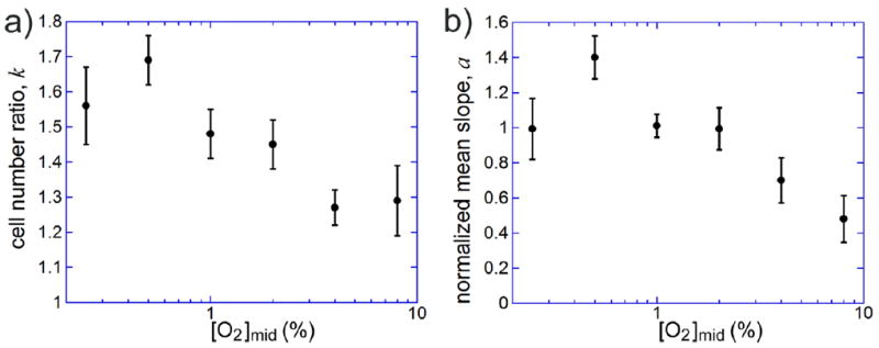
Results of aerotaxis assays on E. coli cells in linear profiles of [O2] at the gas inlet concentrations [O2]A = 0 and [O2]C = 0.5[O2]B, such that [O2] in the middle of the gradient channel, [O2]mid, is equal to [O2]C, and the representative logarithmic slope of the [O2] profile in the gradient channel, Δ[O2]/(w·[O2]mid), is 2.7·10-3 μm-1. The middle ~400 μm wide part of the gradient channel was divided into 14 equal segments along the x-axis, the fractions of E. coli cells in individual segments were measured, the distributions were fitted with straight lines, and the ratios of cell numbers between the last and first segments, k, were calculated from the slopes, a, of the linear fits. The ratio of [O2] between the centers of the last and first segment was ~2.8 in all experiments. (a) Cell number ratio, k, as a function of [O2]mid. The numbers of experiments, N, are 11, 8, 13, 11, 12, and 6 for [O2]mid = 0.25, 0.5, 1, 2, 4, and 8%, respectively, with an average of 7·104 cells interrogated in an experiment. Error bars are SEM. (b) Mean value of the slope of the linear fit, a, normalized to the slope of the fit to the distribution in the gradient with [O2]mid = 1% on the same day of experimentation, as a function of [O2]mid. Error bars are SEM.
In an attempt to better account for the day-to-day variability between the aerotaxis assays, we used a different treatment of the data, with the slopes, a, of the linear fits on each day normalized to the slope of the distribution with [O2]mid = 1% on the same day. The normalized slopes at each [O2]mid were averaged between different days and plotted against [O2]mid (Fig. 4b). The plot of the normalized slopes (Fig. 4b) was largely similar to the plot of the cell number ratios, k, (Fig. 4a). (We note that the zero-aerotaxis baseline for the normalized slopes in Fig. 4b is 0, whereas the baseline for k in Fig. 4a is 1.) However, the error bars (SEM values) in Fig. 4b were smaller, revealing a clearer trend of decay of aerotaxis efficiency with the growth of [O2]mid and a significant difference between [O2]mid of 0.25 and 0.5%. We note that in the biased random walk model, the aerotaxis efficiency, as measured by the value of k or a, is a function of the ratio v/D. Therefore, the reduction of efficiency can be due to reduction of the aerotaxis-driven velocity, v, or increase in the effective diffusivity, D, due to more intense random motion of cells.
We also performed a series of experiments with [O2]mid set at a constant level of 2% (by setting [O2]C to 2%) and with Δ[O2]BA = [O2]B - [O2]A varied between 0, 0.5%, 1%, 2%, and 4%. The resulting gradients had logarithmic slopes Δ[O2]/(w·[O2]mid) of 0, 3.4·10-4, 6.8·10-4, 1.36·10-3, and 2.7·10-3 μm-1, respectively. As in the experiments described in the previous paragraphs, normalized distributions of cells in the 14 segments across the gradient channel were plotted and fitted with straight lines; the slopes, a, were extracted from the fits; the corresponding cell number ratios, k, were calculated; outliers were identified and removed. The data were used to plot the mean values of k vs. Δ[O2]BA with SEM as error bars (Fig. 5a). Also as before, we used an alternative treatment of the data, with slopes, a, of the linear fits to cross-channel cell distributions for all Δ[O2]BA normalized to the slope of the distribution with Δ[O2]BA = 2% on that day, and plotted mean values of the normalized slopes vs. the values of Δ[O2]BA (Fig. 5b). As expected, the efficiency of chemotaxis, as measured by both the cell number ratio, k, and the normalized slope of the cell distribution, monotonically increased with Δ[O2]BA (and with the logarithmic slope of the [O2] profile). Somewhat surprisingly, however, the increase was substantially slower than linear. For Δ[O2]BA changing 8-fold from 0.5% to 4%, k only increased from 1.23 to 1.48, which for a biased random walk with a constant value of D, would correspond to an increase of the cell drift velocity, v, by a factor of <2.
Figure 5.
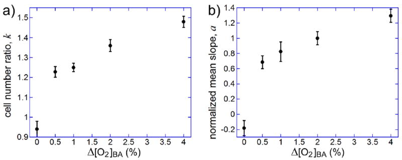
Results of aerotaxis assays on E. coli cells in linear profiles of [O2] at [O2]mid = [O2]C = 2%, with [O2]B + [O2]A = 2[O2]C and Δ[O2]BA = [O2]B - [O2]A varied between 0 and 4%, resulting in constant mid-point gradients of [O2] with logarithmic slopes, Δ[O2]/(w·[O2]mid) = 0.68Δ[O2]BA/(w·[O2]mid), varying between 0 and 2.7·10-3 μm-1. The data analysis was the same as in the experiments with a constant logarithmic slope (Fig. 4). (a) Cell number ratio, k, between the last and the first segment of the gradient channel (~360 μm apart) as a function of Δ[O2]BA. The numbers of experiments, N, are 2, 8, 9, 8, and 8 for Δ[O2]BA = 0, 0.5, 1, 2, and 4%, respectively, with an average of 9·104 cells per experiment. Error bars are SEM. (b) Mean value of the slope of the linear fit, a, normalized to the slope of the fit to the distribution in the gradient with Δ[O2]BA = 2% on the same day of experimentation, as a function of Δ[O2]BA. Error bars are SEM.
DISCUSSION
The aerotaxis assay that we developed and applied is based on the approach proposed of Ref.31, in which a suspension of motile cells is continuously fed into a long channel with a gradient of an attractant across the channel, and the distribution of cells is evaluated at the channel exit. This approach enables achieving a high experimental throughput by collecting data on a large number of different cells, each of which is allowed sufficient time to explore the gradient field. However, this approach is problematic when applied to chemotaxis of motile bacteria in gradients of small-molecule attractants that are not gases, because the diffusivity of small-molecule attractants, Da, is usually comparable with the effective diffusivity, D, of the random motion of motile bacteria (~400 μm2/s for E. coli52). An attractant gradient with a well-defined shape can be readily generated at the gradient channel entrance, using a variety of microfluidic techniques30, 33, 59, 60. Nevertheless, the gradient will continuously deteriorate as the bacterial suspension moves along the channel,30-32 and the deterioration will become severe at a time scale w2 /(2Da) [corresponding to a distance vf w2 /(2Da)], which is comparable to the time Δt = w2 /(2D) [and distance vf w2 /(2D)], required for bacteria to explore the gradient. Therefore, when assays on chemotaxis of motile bacteria are performed in continuous-flow gradient channels, 31, 33 the analysis of the experimental results is always complicated by the variation of the gradient profile along the flow.
Some of the most informative quantitative experiments on bacterial chemotaxis in microfluidic devices were performed in channels without flow, where nearly-linear attractant gradients were generated by molecular diffusion between a source and a sink, by making microfluidic devices out of attractant-permeable hydrogels.34-37 This technique has a relatively low throughput, however, because for distributions of cells across the gradient channels to be completely statistically independent, the interval between consecutive measurements (cell distribution snapshots) should, strictly speaking, be on the order of Δt = w2 /(2D). This interval is ~300 sec for a 500 μm wide channel (and ~200 s for a 400 μm wide channel as in Ref. 36), much longer than the 15 sec time required in our experiments for the content of cells in the field of view to be completely replaced.
Similar to the chemotaxis experiments in microchannels cast in hydrogels, 34-37 the [O2] profile in the aerotaxis experiments is established by diffusion between a source (gas channel network B) and a sink (gas channel network A; with the gas channel network C playing a role of an intermediate). As a result, unlike the continuous-flow experiments on chemotaxis,31, 33 the [O2] profile does not vary along the gradient channel. The continuous-flow aerotaxis experiments in the proposed device are made possible by the high solubility of O2 in the PDMS material of the microfluidic chip (~6 times higher than in water at room temperature) and its relatively high diffusivity in PDMS (~3400 μm2/s) and in water (~2000 μm2/s). The [O2] gradient profile is imbedded in the bulk of the device and is mainly set by the diffusion of O2 through the material of the device rather than through the gradient channel (Fig. 1b). In this respect, the PDMS material of the device is somewhat similar to hydrogel around the gradient channels in the no-flow chemotaxis devices.30, 34-37 However, the solubility and diffusivity of common chemoattractants in hydrogels (about the same as in water and ~500 μm2/s, respectively) are substantially lower that the solubility and diffusivity of [O2] in PDMS. Because of the high diffusivity of [O2] in PDMS and water and ~6 times higher solubility of [O2] in PDMS as compared to water, the time, teq, required for the [O2] profile in a bacterial suspension entering the gradient channel to reach equilibrium is only ~3.5 sec (from numerical simulations), which is two orders of magnitude smaller than the bacterial diffusion time, Δt. Therefore, the continuous flow of bacterial suspension through the gradient channel represents only a minor perturbation to the imposed [O2] gradient.
Because teq ≪ Δt, one can potentially use the device to study the dynamics of establishment of an equilibrium distribution of bacterial cells across the gradient, starting from specific initial conditions. (We note that such type of experiment would be difficult to perform for bacterial chemotaxis in hydrogel-based no-flow microfluidic devices.) To this end, one could confine the bacterial suspension to a certain segment of the channel along the x-axis by hydrodynamically focusing it between two streams of the motility buffer.31, 33 Measurements of the distribution of bacteria along the x-axis at different distances from the inlet (converted to residence times) would then provide direct information on the affective diffusivity, D, and migration velocity, v, of bacteria at different positions, x, in the gradient.
A common problem with bacterial chemotactic assays (both microfluidic and conventional) is the possibility that the imposed gradient profile is modified by cellular metabolism. (As a remedy, non-metabolizable analogues of natural attractants are sometimes used.) By the same token, respiration of E. coli could potentially change an imposed [O2] gradient. In fact, as discussed in the Introduction, in the capillary assays used in some previous works on bacterial aerotaxis, 2, 4, 17, 28 spatial gradients of [O2] are formed as a result of cellular respiration. The O2 consumption of E. coli was reported to increase linearly with the division rate,61, 62 reaching 20 mmol per hour per 1 g of dry mass (20 mmol/hr/g) at a growth rate of ~1 division per hour, which is an upper estimate for E. coli growth rate at room temperature. The concentration of E. coli in the gradient channel in our experiments was ~5×10⁸ mL-1, which for a cell dry mass of ~0.3×10⁻¹² g (taken to be 27% of the live cell mass63) corresponds to a dry mass of ~1.5×10⁻⁴ g/mL and [O2] consumption of 3×10⁻³ mmol/hr/mL or 0.83×10⁻³ mmol/sec/L at 1 division per hour. Given that [O2] = 100% at room temperature (20 °C) and atmospheric pressure corresponds to [O2] of ~1.3 mmol/L in fresh water, the [O2] consumption rate of 0.83×10⁻³ mmol/sec/L is equivalent to 0.064 %/sec. When this [O2] consumption rate in the gradient channel was plugged into our 2D simulation of O2 in the device (cf. Fig. 1b; taking into account the ~6 times lower O2 solubility in water as compared with PDMS) with [O2]A = 0, [O2]B = 2%, and [O2]C = 1%, the perturbation to the [O2] profile caused by the bacterial respiration was found to be minimal. It amounted to a reduction of [O2]mid from 1.0% to 0.97%, with the slope of the [O2] profile remaining unchanged. The perturbation to the [O2] profile was even smaller at larger [O2]B. The perturbation became more significant at lower [O2]B. Nevertheless, reduced levels of [O2] have been found before to reduce the growth rate, to as little as 0.2 divisions per hour (thus likely leading to ~5 times reduced respiration rate) at [O2] = 0.2% at room temperature even in a reach medium, 55 and the low nutrient content of the motility buffer is likely to result in additional reduction of the metabolism and respiration rate. Thus, our estimates and simulations indicate that the bacterial respiration had little effect upon [O2] profiles in the gradient channel.
With microfluidic devices made of monolithic PDMS, it was relatively straightforward to have gas channels both in the plane of the liquid-filled channels and at a height hg ≈ 1.1 mm above it. The flow of an appropriate gas mixture through the out-of-plane gas channels shields the gradient channel from the atmospheric air, facilitating the generation of near-linear [O2] profiles in the gradient channel even at [O2]mid as low as 0.25%. Our simulations also showed that, if pure N2 ([O2] = 0) is ventilated through an extensive network of out-of-plane gas channels, it would create a nearly O2-free (anoxic) region at the cover glass with an area comparable to that of the out-of-plane gas channel network. This approach could be used to create O2-free conditions, which are favorable for photostability of fluorescent dyes56 and for anaerobic cell cultures, without significantly compromising the structural properties of microfluidic channels near the cover glass (because hg is relatively large).
Our numerical simulations also indicate that modified versions of the gas channel networks can enable the generation of various exponential profiles of [O2] across a liquid-filled gradient channel (see Supplementary Information). To this end, the internal edges of the in-plane gas channel networks A and B are positioned asymmetrically with respect to the gradient channel, and a proper hg is selected (Supplementary Fig. S-4). In three specific examples we considered (Supplementary Fig. S-4a-c), the gas channel arrangements produced near-perfect exponential profiles with logarithmic slopes, d ln([O2]) / dx, of ~0.002, ~0.004, and ~0.008 μm-1, all at [O2]A and [O2]C both set to 0. We note that the slope of ~0.008 μm-1 is ~3 times greater than the maximal representative logarithmic slope of 0.0027 μm-1 produced by the device in Fig. 1. In addition, the slope of ~0.008 μm-1 corresponds to an ~50-fold variation of [O2] across a 500 μm wide gradient channel, as compared to the ~5-fold variation of [O2] in the device in Fig. 1. Importantly, the logarithmic slopes in the devices in Supplementary Fig. S-4 remain unchanged when [O2]B is varied, as long as [O2]A and [O2]C both remain zero, whereas the actual value of [O2] at given x is proportional to [O2]B. Therefore, the actual ranges of [O2] in the gradient channels of the devices in Supplementary Fig. S-4 can be readily adjusted by varying a single parameter, [O2]B. Based on the results in Fig. 5, [O2] profiles with greater logarithmic slopes are expected to elicit stronger aerotactic responses. In addition, a profile with a large logarithmic slope covers a broad range of [O2] and could thus be efficiently used for testing the preferred levels of [O2] of different bacteria.
There are several conclusions that can be drawn from the results of our aerotaxis experiments on E. coli (Fig. 4-5). First, in a range of [O2] from 0.08% (lowest in the 0 – 0.5% profile) to 11.5% (highest in the 0 – 16% profiles), E. coli cells always prefer regions with the highest available [O2] (Fig. 4). This result contradicts some previous unpublished reports that E. coli prefer O2 concentrations of 50 or 40 μM, 2, 14 which at room temperature correspond to [O2] = 3 – 4%. Significant positive aerotactic response to the linear profile with [O2]mid = 8% (Fig. 4), which extends from 3.5% to 11.5% of [O2], does not agree very well with the previous report on a very low value of [O2] of 0.07% (0.8 μM) eliciting half-maximal positive (attractive) aerotactic response in E. coli.28 On the other hand, the positive aerotaxis in the [O2] = 3.5% – 11.5% profile is consistent with a value of ~80% (1.0 mM) for [O2] causing half-maximal negative (repulsive) aerotactic response starting from an initial [O2] of 15% in the RP437 strain of E. coli. 28 Furthermore, the lowest value of [O2] of ~33%, to which a negative aerotactic response starting from [O2] = 15% was observed in Ref. 28, does not contradict our experimental findings either. Second, as expected, at a given average [O2] ([O2]mid in Fig. 5), the efficiency of aerotaxis is an increasing function of [O2] gradient, d[O2] / dx. Surprisingly, however, the efficiency of aerotaxis, as measured by both the slope, a, of the cell distribution and the estimated cell migration velocity, v, increases with d[O2] / dx substantially slower than linearly. So, in the framework of a biased random walk model, assuming a constant effective diffusivity, D, the apparent migration velocity, v, grows by a factor <2, when d[O2] / dx is increased as much as 8-fold (Fig. 5). Third, in linear profiles with a constant mean logarithmic slope d ln([O2]) / dx, the efficiency of aerotaxis (as measured by the steady-state distributions in Fig. 4) significantly decreases with the average concentration, [O2]mid, in a range of [O2]mid from 0.5% to 8%. (In the biased random walk model, this apparent reduction of aerotactic efficiency could be due to reduction of v or growth of D with [O2]mid.) This reduction of the aerotaxis efficiency with [O2]mid is consistent with a suggestion that RP437 E. coli has its preferred range at [O2] somewhere between 12 and 33%. It is also worth noting that the preferred level of [O2] is expected to depend on the exact conditions in the bacterial culture prior to the aerotaxis assay.
Conclusions
The proposed microfluidic device generates robust near-linear profiles of [O2] and enables high-throughput experiments on aerotaxis of swimming bacteria in a continuous flow, where distributions of cells in a steady gradient of [O2] are measured after cells are allowed sufficient time to explore the gradient. The device can also potentially be used to explore the dynamics of development of a steady state distribution from various initial distributions of cells in the gradient, thus enabling more detailed studies of bacterial aerotaxis. A modification of the proposed design would enable the application of exponential profiles of [O2], making it possible to present cells with steeper gradients and measure their responses in broader ranges of [O2] in a single experiment. High-throughput experiments in steady gradients of [O2] are enabled by a high O2-permeability of the PDMS material of the microfluidic device, making bacterial aerotaxis assays to some extent easier to perform than chemotaxis assays. The experiments on E. coli aerotaxis presented here are the first detailed study of aerotaxis of any bacterial species in stable well-defined gradients of [O2]. The study provides new quantitative data on E. coli aerotaxis in different linear profiles, in particular, the dependence of the efficiency of aerotaxis on the gradient and mean value of [O2]. The technique of shielding the gradient channel form the atmosphere with an out-of-plane gas channel network implemented in the device enables generation of gradients with low mean values of [O2]. Therefore, in addition to more extensive experiments on aerotaxis of E. coli and other aerobic bacteria, the device and technique can be used to study the behavior of microaerobic organisms and could potentially be applied to anaerobic bacteria.
Supplementary Material
Acknowledgments
We are grateful to Prof. Victor Sourjik for his encouragement and guidance on the bacterial chemotaxis and help with E. coli cultures. We thank Prof. J.S. Parkinson for providing us with E. coli RP437 strain. The work was supported by NIH Grants PO1 GM078586 and R01 GM084332.
References
- 1.Engelmann T. Pflugers Arch Gesammte Physiol. 1881;25:285–292. [Google Scholar]
- 2.Taylor BL, Zhulin IB, Johnson MS. Annu Rev Microbiol. 1999;53:103–128. doi: 10.1146/annurev.micro.53.1.103. [DOI] [PubMed] [Google Scholar]
- 3.Baracchini O, Sherris JC. Journal Of Pathology And Bacteriology. 1959;77:565–574. doi: 10.1002/path.1700770228. [DOI] [PubMed] [Google Scholar]
- 4.Wong LS, Johnson MS, Zhulin IB, Taylor BL. J Bacteriol. 1995;177:3985–3991. doi: 10.1128/jb.177.14.3985-3991.1995. [DOI] [PMC free article] [PubMed] [Google Scholar]
- 5.Rebbapragada A, Johnson MS, Harding GP, Zuccarelli AJ, Fletcher HM, Zhulin IB, Taylor BL. PNAS. 1997;94:10541–10546. doi: 10.1073/pnas.94.20.10541. [DOI] [PMC free article] [PubMed] [Google Scholar]
- 6.Czirok A, Janosi IM, Kessler JO. J Exp Biol. 2000;203:3345–3354. doi: 10.1242/jeb.203.21.3345. [DOI] [PubMed] [Google Scholar]
- 7.Yu HS, Saw JH, Hou SB, Larsen RW, Watts KJ, Johnson MS, Zimmer MA, Ordal GW, Taylor BL, Alam M. FEMS Microbiol Lett. 2002;217:237–242. doi: 10.1111/j.1574-6968.2002.tb11481.x. [DOI] [PubMed] [Google Scholar]
- 8.Zhang W, Olson JS, Phillips GN. Biophys J. 2005;88:2801–2814. doi: 10.1529/biophysj.104.047936. [DOI] [PMC free article] [PubMed] [Google Scholar]
- 9.Laszlo DJ, Taylor BL. J Bacteriol. 1981;145:990–1001. doi: 10.1128/jb.145.2.990-1001.1981. [DOI] [PMC free article] [PubMed] [Google Scholar]
- 10.Glagolev AN, Sherman MY. FEMS Microbiol Lett. 1983;17:147–150. [Google Scholar]
- 11.Armitage JP. Annual Review Of Physiology. 1992;54:683–714. doi: 10.1146/annurev.ph.54.030192.003343. [DOI] [PubMed] [Google Scholar]
- 12.Bibikov SI, Biran R, Rudd KE, Parkinson JS. J Bacteriol. 1997;179:4075–4079. doi: 10.1128/jb.179.12.4075-4079.1997. [DOI] [PMC free article] [PubMed] [Google Scholar]
- 13.Bibikov SI, Barnes LA, Gitin Y, Parkinson JS. PNAS. 2000;97:5830–5835. doi: 10.1073/pnas.100118697. [DOI] [PMC free article] [PubMed] [Google Scholar]
- 14.Zhulin IB, Johnson MS, Taylor BL. Biosci Rep. 1997;17:335–342. doi: 10.1023/a:1027340813657. [DOI] [PubMed] [Google Scholar]
- 15.Okon Y, Cakmakci L, Nur I, Chet I. Microb Ecol. 1980;6:277–280. doi: 10.1007/BF02010393. [DOI] [PubMed] [Google Scholar]
- 16.Grishanin RN, Chalmina II, Zhulin IB. J Gen Microbiol. 1991;137:2781–2785. [Google Scholar]
- 17.Zhulin IB, Bespalov VA, Johnson MS, Taylor BL. J Bacteriol. 1996;178:5199–5204. doi: 10.1128/jb.178.17.5199-5204.1996. [DOI] [PMC free article] [PubMed] [Google Scholar]
- 18.Alexandre G, Greer SE, Zhulin IB. J Bacteriol. 2000;182:6042–6048. doi: 10.1128/jb.182.21.6042-6048.2000. [DOI] [PMC free article] [PubMed] [Google Scholar]
- 19.Stephens BB, Loar SN, Alexandre G. J Bacteriol. 2006;188:4759–4768. doi: 10.1128/JB.00267-06. [DOI] [PMC free article] [PubMed] [Google Scholar]
- 20.Bible AN, Stephens BB, Ortega DR, Xie ZH, Alexandre G. J Bacteriol. 2008;190:6365–6375. doi: 10.1128/JB.00734-08. [DOI] [PMC free article] [PubMed] [Google Scholar]
- 21.Cypionka H. Annual Review Of Microbiology. 2000;54:827–848. doi: 10.1146/annurev.micro.54.1.827. [DOI] [PubMed] [Google Scholar]
- 22.Johnson MS, Zhulin IG, Gapuzan MER, Taylor BL. J Bacteriol. 1997;179:5598–5601. doi: 10.1128/jb.179.17.5598-5601.1997. [DOI] [PMC free article] [PubMed] [Google Scholar]
- 23.Eschemann A, Kuhl M, Cypionka H. Environ Microbiol. 1999;1:489–494. doi: 10.1046/j.1462-2920.1999.00057.x. [DOI] [PubMed] [Google Scholar]
- 24.Mazzag BC, Zhulin IB, Mogilner A. Biophys J. 2003;85:3558–3574. doi: 10.1016/S0006-3495(03)74775-4. [DOI] [PMC free article] [PubMed] [Google Scholar]
- 25.Krekeler D, Teske A, Cypionka H. FEMS Microbiol Ecol. 1998;25:89–96. [Google Scholar]
- 26.Schweinitzer T, Josenhans C. Arch Microbiol. 2010;192:507–520. doi: 10.1007/s00203-010-0575-7. [DOI] [PMC free article] [PubMed] [Google Scholar]
- 27.Boin MA, Hase CC. FEMS Microbiol Lett. 2007;276:193–201. doi: 10.1111/j.1574-6968.2007.00931.x. [DOI] [PubMed] [Google Scholar]
- 28.Shioi J, Dang CV, Taylor BL. J Bacteriol. 1987;169:3118–3123. doi: 10.1128/jb.169.7.3118-3123.1987. [DOI] [PMC free article] [PubMed] [Google Scholar]
- 29.Bespalov VA, Zhulin IB, Taylor BL. PNAS. 1996;93:10084–10089. doi: 10.1073/pnas.93.19.10084. [DOI] [PMC free article] [PubMed] [Google Scholar]
- 30.Ahmed T, Shimizu TS, Stocker R. Integr Biol. 2010;2:604–629. doi: 10.1039/c0ib00049c. [DOI] [PubMed] [Google Scholar]
- 31.Mao HB, Cremer PS, Manson MD. PNAS. 2003;100:5449–5454. doi: 10.1073/pnas.0931258100. [DOI] [PMC free article] [PubMed] [Google Scholar]
- 32.Ahmed T, Stocker R. Biophys J. 2008;95:4481–4493. doi: 10.1529/biophysj.108.134510. [DOI] [PMC free article] [PubMed] [Google Scholar]
- 33.Englert DL, Manson MD, Jayaraman A. Appl Environ Microbiol. 2009;75:4557–4564. doi: 10.1128/AEM.02952-08. [DOI] [PMC free article] [PubMed] [Google Scholar]
- 34.Diao JP, Young L, Kim S, Fogarty EA, Heilman SM, Zhou P, Shuler ML, Wu MM, DeLisa MP. Lab Chip. 2006;6:381–388. doi: 10.1039/b511958h. [DOI] [PubMed] [Google Scholar]
- 35.Cheng SY, Heilman S, Wasserman M, Archer S, Shuler ML, Wu MM. Lab Chip. 2007;7:763–769. doi: 10.1039/b618463d. [DOI] [PubMed] [Google Scholar]
- 36.Kalinin YV, Jiang LL, Tu YH, Wu MM. Biophys J. 2009;96:2439–2448. doi: 10.1016/j.bpj.2008.10.027. [DOI] [PMC free article] [PubMed] [Google Scholar]
- 37.Ahmed T, Shimizu TS, Stocker R. Nano Lett. 2010;10:3379–3385. doi: 10.1021/nl101204e. [DOI] [PMC free article] [PubMed] [Google Scholar]
- 38.Zigmond SH. J Cell Biol. 1977;75:606–616. doi: 10.1083/jcb.75.2.606. [DOI] [PMC free article] [PubMed] [Google Scholar]
- 39.Paliwal S, Iglesias PA, Campbell K, Hilioti Z, Groisman A, Levchenko A. Nature. 2007;446:46–51. doi: 10.1038/nature05561. [DOI] [PubMed] [Google Scholar]
- 40.Herzmark P, Campbell K, Wang F, Wong K, El-Samad H, Groisman A, Bourne HR. PNAS. 2007;104:13349–13354. doi: 10.1073/pnas.0705889104. [DOI] [PMC free article] [PubMed] [Google Scholar]
- 41.Fuller D, Chen W, Adler M, Groisman A, Levine H, Rappel WJ, Loomis WF. PNAS. 2010;107:9656–9659. doi: 10.1073/pnas.0911178107. [DOI] [PMC free article] [PubMed] [Google Scholar]
- 42.Vollmer AP, Probstein RF, Gilbert R, Thorsen T. Lab Chip. 2005;5:1059–1066. doi: 10.1039/b508097e. [DOI] [PubMed] [Google Scholar]
- 43.Allen JW, Bhatia SN. Biotechnol Bioeng. 2003;82:253–262. doi: 10.1002/bit.10569. [DOI] [PubMed] [Google Scholar]
- 44.Pinelis M, Shamban L, Jovic A, Maharbiz MM. Biomed Microdevices. 2008;10:807–811. doi: 10.1007/s10544-008-9195-2. [DOI] [PubMed] [Google Scholar]
- 45.Mehta G, Mehta K, Sud D, Song JW, Bersano-Begey T, Futai N, Heo YS, Mycek MA, Linderman JJ, Takayama S. Biomed Microdevices. 2007;9:123–134. doi: 10.1007/s10544-006-9005-7. [DOI] [PubMed] [Google Scholar]
- 46.Higgins JM, Eddington DT, Bhatia SN, Mahadevan L. PNAS. 2007;104:20496–20500. doi: 10.1073/pnas.0707122105. [DOI] [PMC free article] [PubMed] [Google Scholar]
- 47.Park J, Bansal T, Pinelis M, Maharbiz MM. Lab Chip. 2006;6:611–622. doi: 10.1039/b516483d. [DOI] [PubMed] [Google Scholar]
- 48.Adler M, Polinkovsky M, Gutierrez E, Groisman A. Lab Chip. 2010;10:388–391. doi: 10.1039/b920401f. [DOI] [PMC free article] [PubMed] [Google Scholar]
- 49.Oppegard SC, Nam KH, Carr JR, Skaalure SC, Eddington DT. Plos One. 2009:4. doi: 10.1371/journal.pone.0006891. [DOI] [PMC free article] [PubMed] [Google Scholar]
- 50.Lo JF, Sinkala E, Eddington DT. Lab Chip. 2010;10:2394–2401. doi: 10.1039/c004660d. [DOI] [PMC free article] [PubMed] [Google Scholar]
- 51.Li N, Luo CX, Zhu XJ, Chen Y, Qi OY, Zhou LP. Microelectron Eng. 2011;88:1698–1701. [Google Scholar]
- 52.Berg HC, Turner L. Biophys J. 1990;58:919–930. doi: 10.1016/S0006-3495(90)82436-X. [DOI] [PMC free article] [PubMed] [Google Scholar]
- 53.Berg HC. Random walks in biology. Princeton University Press; 1993. [Google Scholar]
- 54.Lam RHW, Kim M-C, Thorsen T. Anal Chem. 2009;81:5918–5924. doi: 10.1021/ac9006864. [DOI] [PMC free article] [PubMed] [Google Scholar]
- 55.Polinkovsky M, Gutierrez E, Levchenko A, Groisman A. Lab Chip. 2009;9:1073–1084. doi: 10.1039/b816191g. [DOI] [PubMed] [Google Scholar]
- 56.Lemke EA, Gambin Y, Vandelinder V, Brustad EM, Liu HW, Schultz PG, Groisman A, Deniz AA. JACS. 2009;131:13610. doi: 10.1021/ja9027023. [DOI] [PMC free article] [PubMed] [Google Scholar]
- 57.Merkel TC, Bondar VI, Nagai K, Freeman BD, Pinnau I. J Polym Sci, Part B: Polym Phys. 2000;38:415–434. [Google Scholar]
- 58.Parkinson JS. J Bacteriol. 1978;135:45–53. doi: 10.1128/jb.135.1.45-53.1978. [DOI] [PMC free article] [PubMed] [Google Scholar]
- 59.Jeon NL, Dertinger SKW, Chiu DT, Choi IS, Stroock AD, Whitesides GM. Langmuir. 2000;16:8311–8316. [Google Scholar]
- 60.Campbell K, Groisman A. Lab Chip. 2007;7:264–272. doi: 10.1039/b610011b. [DOI] [PubMed] [Google Scholar]
- 61.Schulze KL, Lipe RS. Archiv Fur Mikrobiologie. 1964;48:1–20. doi: 10.1007/BF00406595. [DOI] [PubMed] [Google Scholar]
- 62.Calhoun MW, Oden KL, Gennis RB, Demattos MJT, Neijssel OM. Journal Of Bacteriology. 1993;175:3020–3025. doi: 10.1128/jb.175.10.3020-3025.1993. [DOI] [PMC free article] [PubMed] [Google Scholar]
- 63.Winkler HH, Wilson TH. Journal Of Biological Chemistry. 1966;241:2200–2211. [PubMed] [Google Scholar]
Associated Data
This section collects any data citations, data availability statements, or supplementary materials included in this article.