

Abstract
The response of complex molecules to sequences of femtosecond infrared pulses provides a unique window into their structure, dynamics and fluctuating environments, as projected into the vibrational degrees of freedom. In this review we survey the basic principles of these novel two dimensional infrared (2DIR) analogues of multidimensional NMR. The perturbative approach for computing the nonlinear optical response of coupled localized chromophores is introduced and applied to the amide backbone transitions of protein, liquid water, membrane lipids, and amyloid fibrils. The signals are analyzed using classical MD simulations combined with an effective fluctuating Hamiltonian for coupled localized anharmonic vibrations whose dependence on the local electrostatic environment is parameterized by an ab initio map. Several simulation protocols. Including the Cumulant expansion of Gaussian Fluctuation (CGF), a quasiparticle scattering approach (NEE), the Stochastic Liouville Equations (SLE), and Direct Numerical Propagation are surveyed. These are implemented in a code SPECTRON that interfaces with standard electronic structure and molecular mechanisms MD codes. Chirality-induced techniques which dramatically enhance the resolution are demonstrated. Signatures of conformational and hydrogen bonding fluctuations, protein folding, and chemical exchange processes are discussed.
I. Introduction
The structure and function of biomolecules are intimately connected; this is one of the central paradigms of structural biology[1]. Predicting protein structures requires understanding the interactions and driving forces which cause them to fold from a disordered, random-coiled, state into a unique native structure. Exploring the folding mechanism in detail requires techniques that can monitor the structures with adequate temporal and spatial resolution. X-ray crystallography can determine the static atomic-resolution structure [2]. Time-resolved small angle X-ray scattering gives mainly the radius of gyration with up to picosecond time-resolution [3-6] Three-dimensional atomic-resolution structures can be determined using nuclear magnetic resonance (NMR) [7, 8] on time scales longer than the radiowave period (microsecond) [8]. Higher temporal resolution is required for monitoring many elementary biophysical processes, for example the R-helix formation [9], which has a hundreds nanosecond timescale. Nanosecond to picosecond processes may sometimes be probed through the frequency dependence of NMR relaxation rates [10]. Such measurements are indirect and their interpretation is model-dependent. Time-resolved x-ray diffraction provides picosecond snapshots of structures in crystals [11]. Ultrafast electron pulses are being developed as well for time resolved electron diffraction applications [12, 13].
Over the past decade, time-resolved infrared spectroscopy carried out with 20-100 fs laser pulses has emerged as a powerful tool in the investigation of protein folding [14], thanks to fast laser-triggering and the fairly localized nature of vibrational transitions [14-20]. The coherent techniques surveyed here record the molecular response to sequences of pulses, and provide a multidimensional view of their structure. Multidimensional optical techniques are analogues of their NMR counterparts but with greatly-improved temporal resolution [21, 22]. This and other differences are summarized in Table I [23-25]. NMR experiments are performed with strong pulses which move the entire spin population. Pulse sequences involving hundreds of pulses are then possible. In order to avoid photochemical processes infrared studies use weak pulses which only excite a small fraction of the molecules. This limits the applicability to few pulses, since each additional pulse results in a considerable reduction in the signal. The signals can then be calculated perturbatively order by order in the incoming fields. The directionality of the signal (phase matching) stems from the fact that the sample is much larger than the optical wavelength. In NMR the opposite limit holds: The signal is thus isotropic. However, the directional information may be retrieved by modifying the phases of the pulses (phase cycling). The anharmonic effective Hamiltonian necessary for 2DIR simulations is complex and requires extensive electronic structure calculations. The spin Hamiltonians is NMR, in contrast, are known and universal, greatly simplifying the simulations and analysis of signals. The dipole moments in NMR are aligned in parallel by the strong magnetic field. In contrast, the specific orientations of infrared dipoles have useful structural information that can be retrieved by varying the pulse polarizations. NMR has a remarkable structural resolution unmatched by infrared signals. However, 2DIR provides a different window with complementary information. A heterodyne-detected 2DIR experiment (Fig.1) involves the interaction of three laser pulses with wave vectors k1,k2, k3, (in chronological order) with the peptide. A coherent signal field is then generated along one of the phase-matching direction: ks = ± k1±k2±k3 where all molecules are excited in phase and detected by interference with a 4th “Local-oscillator” pulse with the desired wavevector ks.
Table I. Comparison of coherent NMR and IR technique.
| NMR | IR | |
|---|---|---|
| Frequency | MHZ | 1012-1013 Hz |
| Time Resolution | microsecond | Femtosecond |
| Hamiltonian | Spin Hamiltonian. Few universal parameters. Easier to invert spectra to get structures | Anharmonic vibrational Hamiltonian, Requires electronic structure calculation. Many parameters. Inversion of signals is more complex |
| Transition Dipoles | All dipoles of the same nucleus are equal and aligned, Gyromagnetic ratio. Pulse polarizations and spin states transform by rotating the sample | Varying dipoles. Arbitrary orientation. Many independent parameters for the dipole |
| Pulse intensity | Strong saturating pulses. All spins excited, multiple pulse sequences possible. | weak, only few molecules are excited,sequences with few pulses possible. |
| Modeling | The Bloch picture | Susceptibilities and response functions |
| Directionality of signal | Wavelength λ ≫ sample size, kr ≪ l,Signal is isotropic in space. Pathway selection by phase cycling | λ ≪ sample size, kr ≫ 1, signal is highly directional. Pathway selection by spatial phase matching |
| Target degrees of freedom | spins | Molecular vibrations |
| Temperature | high compared to frequencies, Simplifies calculations | low compared to frequencies, Calculation more complicated |
| Phase control of pulses | Easy 7 | Becomes feasible using pulse shaping |
Fig. 1.

Pulse configuration for a heterodyne detected multidimensional four-wave mixing experiment. Signals are recorded vs. the three time delays t1, t2, t3, and t4 and displayed as 2D correlation plots involving two of the time delays, holding the third fixed.(see Eq.14)
The signal S(t3, t2, t1) is given as the intensity change of the local-oscillator field induced by the interactions with the field irradiated by the nonlinear polarization. Its parametric dependence on the time intervals between pulses carries a wealth of information. 2DIR signals are typically displayed as two-dimensional correlation plots with respect to two of these intervals, say t1 and t3, holding the third (t2) fixed. Since such plots are highly-oscillatory, the signal is double Fourier transformed with respect to the two desired time variables to generate a frequency/frequency correlation plot such as S(Ω1, t2, Ω3) where Ω1 and Ω3 are the frequency conjugates to t1 and t3 (Fig. 1). Heterodyne-detection allows to record the signal field itself (both amplitude and phase). We can thus display both the real (in-phase) and the imaginary (out-of-phase) components of the response. The signatures of coupled vibrational modes are new resonances, cross-peaks, whose intensities and profiles give direct zero-background signatures of the correlations between transitions. These are background-free features that vanish for uncoupled vibrations. Such correlation plots of dynamical events taking place during controlled evolution periods can be interpreted in terms of multipoint correlation functions. These carry considerably more information than the two-point functions of linear spectroscopy, and therefore have the capacity to distinguish between possible models whose 1D responses are virtually identical. In Fig-2, we present simulated 2D photon echo spectra of two coupled vibrations. The diagonal peaks at (−2000,2000) and (−2100,2100) resemble the linear absorption. The cross peaks at (−2000,2100) and (−2100,2000) reveals information about the couplings between the two modes. The 2D lineshapes are very sensitive to frequency fluctuation time scales and the degree of correlations and provide valuable information about the fluctuating environment. Fast fluctuations (right panel) show circular diagonal peaks (homogeneous broadening) whereas slow fluctuations (left panel) yield elongated lineshapes. In addition the figures show strong variations of the cross peaks with the degree of correlations (as can be seen by comparing the left and middle panel). Bandshape analysis of 2D photon echoes of solute-solvent complexes showed the longer time scale of the slowest component in the mixed solvents than in pure solvent. This was ascribed to composition variations of the first solvent shell [26]. Such fine details are not available from 1D measurements.
Fig. 2.

[(Top) 2D photon echo spectra of two coupled vibrations in the phase-matching direction kI = -k1+k2+k3. Ω1 and Ω3 are the Fourier conjugate variables to t1 and t3. (Left) The frequency fluctuations of the two modes are slow and anti-correlated. (Center) Slow and correlated. (Right) Fast and anti-correlated. (Adapted from ref [27].) (Bottom) Linear absorptions for the three models.
Pump-probe (also known as transient absorption) is the simplest nonlinear experiment, both conceptually and technically since it only involves two laser pulses: the pump and the probe, and requires no phase-control. Typically, the two pulses are temporally well-separated. The system first interacts with the pump then with the probe. The difference between the probe transmission with and without the pump, reveals information about structural changes and energy-transport taking place during the delay between the two pulses. The Photon-echo signal generated in the direction ks = −k1 + k2 + k3 is another widely-used technique [28]. The excitations generated in the molecule during t1 and t3 acquire an opposite phase, exactly canceling inhomogeneous broadening in the signal and opening a window into motions and relaxation timescales. This is not possible with 1D techniques such as linear absorption. Frequency-domain experiments involving longer pulses, which combine infrared and Raman techniques have been carried out [29].
2D technique has been applied to many fields of physics, physical chemistry and physical biology, including exploring the equilibrated structure of biomolecules, monitoring ps-ns peptide folding dynamics, studying the hydrogen bonding structure and dynamics in liquid water, monitoring the electrostatic environment and its fluctuations around a chromophore, investigating the vibrational energy transfer pathways and retrieving useful information on reaction rates, mechanisms and yields. A brief survey of these applications is presented in sectionII.
Fast peptide-folding has been extensively studied by Monte Carlo (MC) or Molecular Dynamics (MD) simulations [30-37]. Simple lattice models [35, 36] help develop the big physical picture of the folding events, while all-atom molecular dynamics simulations [32, 37] provide more realistic and detailed structural and dynamical information. Computational power restricts such calculations to a few tens of nanosecond trajectories. A 1998 study had reported the protein folding with explicit representation of water for 1 microsecond [38]. The direct simulation of protein folding is usually too expensive [39-41]. However, MD simulations are gradually acquiring the capacity to unravel the folding mechanism of peptides and small proteins, thanks to (i) the design of simple model peptides that mimic protein complexity, yet sufficiently small to allow detailed simulations [33, 40, 42-44] and (ii) the development and implementation of powerful simulation algorithms [45] with improved sampling of rare events [46, 47]. Since the visualization of folding processes strongly depends on simulations, it is highly desirable to perform experiments on time scales accessible to computer simulations. 2DIR and atomistic level MD simulations have overlapping timescale. Thus developing MD protocols for simulating 2DIR signals can help assign 2DIR features, and unravel the underlying motions. At the same time one can test the quality of different MD force fields by comparing the predicted 2DIR signatures of different folding pathways with experiment.
The state-of-the-art computational techniques currently employed in the modeling of 2DIR signals of biomolecules will be surveyed in this article [48-55]. The amide vibrations of peptides [55-57], can be described by the Frenkel exciton model originally developed to describe coupled localized transitions of oligomers or polymers made out of similar repeat units. The necessary parameters can be obtained from electronic structure calculations of individual chromophores, rather than the whole system, greatly reducing the computational cost. The spectrum consists of well-separated bands of energy levels representing single excitations, double excitations, etc. The molecular Hamiltonian conserves the number of excitations; only the optical fields can induce interband transitions. The lowest (single-exciton) manifold is accessible by linear optical techniques such as absorption and CD, while the doubly excited (two-exciton) and higher manifolds only show up in nonlinear spectroscopies. A high level fluctuating excitonic Hamiltonian for polypeptides is presented in Section II. In section IV we introduce the response function approach for simulating the signals. The modeling of the coherent vibrational response involves the following key steps:
A sequence of protein and solvent configurations is generated by an MD trajectory using existing Molecular Mechanics force fields such as CHARMM [58], GROMOS [59], and AMBER [60].
A fluctuating effective vibrational-exciton Hamiltonian, Ĥs (t), and the transition dipole matrix μ (t) for the relevant states, is constructed for each configuration. This must be a higher-level anharmonic Hamiltonian, than the molecular mechanics force fields used in step (1) to model the structure.
Four-point correlation functions of transition dipoles are calculated. Both orientational [61] and temporal averaging are necessary in order to account for fluctuations.
The response functions are calculated by taking the proper combinations of the four point correlation functions representing the quantum Liouville-space pathways relevant for the chosen technique.
Step 1 is well developed and documented and can use the broad arsenal of available algorithms and software packages. In this sum-over-state (SOS) approach [62] the optical fields induce transitions between system eigenstates, and the nonlinear response is attributed to the anharmonicity of the system (note that harmonic vibrations are linear, their nonlinear response vanishes by interference between quantum pathways). This method is practical for small peptides (as an example, the amide I bands of a peptide with less than 30 residues).
Section II presents a brief survey of the history of coherent multidimentional spectroscopy. This section may be shipped without affecting the clarity of the presentation. Section III we review the protocols for constructing the fluctuating excitonic Hamiltonian for the peptide amide bands. The theoretical framework of modeling the nonlinear optical signal is introduced in section IV, we further discuss a simple exactly soluable Gaussian fluctuation model. The stochastic Liouville equations approach for describing chemical exchange and spectral diffusion by incorporating external collective bath coordinates is introduced in Sec.V. Applications of this approach to the hydrogen bonding fluctuation dynamics in water as observed in the OH stretch of HOD in D20 are given in Sec. VI. A different protocol [48, 62, 63] more suitable for large biomolecules such as globular proteins or membrane systems is described in Sec. VII. The signal is connected to the scattering of single excitations (quasiparticles) rather than transitions between states. The quasiparticle expressions which scale more favorably with size can be derived by using equations of motion, the Nonlinear Exciton Equations (NEE) [64]. In Sec.VIII we demonstrate how a specific choice of the signal wavevector can reveal double excitations (double-quantum-coherence) which provide a different window for structure. Chirality-induced signals, 2D analogues of circular dichroism, aimed at improving the resolution of 2DIR signals by exploiting the chirality of peptides, are presented in sec IX. Amyloid fibrils are aggregates formed by misfolded peptides associated with several human diseases such as Alzheimer disease. Their toxicities strongly depend on their structures. 2DIR simulations described in sec X are very promising for retrieving structural information, not available from other techniques. A summary and future outlook of multidimensional techniques are presented in Sec. XI.
II. History of Multidimensional Vibrational Spectroscopy
Infrared absorption, provides a one dimensional (1D) projection of molecular information onto a single frequency axis, through the linear polarization induced in the sample to first order in the field. Higher-order polarizations, and more complex molecular events, can be revealed by various nonlinear spectroscopic techniques. The coherent techniques [65, 66] such as fluorescence, spontaneous Raman and pump probe which are incoherent and independent on the phases of the laser pulses. This is in contrast to the modeling of nonlinear spectra is simplified considerably when the relaxation rates of frequency fluctuations (Λ) are either very fast or very slow compared to their magnitude (Δ). In that case they can be incorporated phenomenologically as homogeneous (Δ/Λ ≪ 1) or inhomogeneous (Δ/Λ ≫ 1) broadening respectively. Picosecond, electronically off-resonant, Coherent anti-Stokes Raman Spectroscopy (CARS) measurements of vibrational dephasing performed in the seventies were believed to have the capacity to distinguish between the two broadening mechanisms [67, 68]. This is known to be the case for the photon echo technique [69]. By formulating the problem in terms of multipoint correlation functions of the electric polarizability, Loring and Mukamel [70] have shown that this is not the case. The key lesson was that optical signals should be classified by their dimensionality, i.e., the number of externally-controlled time intervals rather than by the nonlinear order in the field. Both photon echo and electronically off-resonant time resolved CARS signals are third order in the external fields. However, the latter only has one control time variable t2 (see Fig. 1). The other two times t1 and t3 are very short, as dictated by the Heisenberg uncertainty relation and carry no molecular information. The technique is thus one-dimensional, (1D) carries identical information to the spontaneous raman and can not in principle distinguish between the two mechanisms. Based on this analysis a 2D Raman analogue of the photon echo will require seven rather than three pulses. Such experiments were carried out subsequently [71-73] Closed expressions derived for the multipoint correlation functions of a multilevel system whose frequencies undergo stochastic Gaussian fluctuations [74, 75] had paved the way for the multidimensional simulations of such spectra [76]. Tanimura and Mukamel [77] subsequently proposed a simpler, five-pulse, impulsive off resonant Raman technique and showed how it can be interpreted using 2D frequency/frequency correlation plots. This work which pointed out the analogy with multidimensional NMR had triggered an intense experimental and theoretical activity. Experiments performed on low frequency (∼300 cm−1) intermolecular vibrations in liquid CS2 [78-87] were initially complicated by cascading effects (sequences of lower order processes). These were eventually resolved [88]. Applications to liquid formaimde were reported as well [89]. The same idea was then proposed [48, 65, 90] and implemented for vibrational spectroscopy in the infrared [57, 91-93] and for electronic spectroscopy in the visible. [94-97] Infrared techniques require fewer pulses, since each transition involves a single field, rather than two for Raman. The necessary control of the phase of some or all laser pulses, which is straightforward for radiowaves (NMR) is considerably more challenging for higher frequencies.
2DIR can reveal the equilibrated structure of biomolecules. The first frequency-frequency 2D IR measurement was carried out by Hamm and Hochstrasser [98], who employed a pump probe technique with two infrared pulses with a narrow (∼10 cm−1) pump and a broad (130 cm−1) probe. The signal field was dispersed in a spectrometer and recorded vs the pump and the dispersed signal frequencies. This study demonstrated how the cross peaks can be used to investigate the structures of small peptides [99]. The diagonal peaks reveal the energies of the localized carbonyl C=O vibrational mode, while the cross peaks are directly related to the couplings between those modes which depend on the peptide structure. The cross peak intensities and anisotropies of a cyclic rigid penta-peptide were connected to 3D structure with the help of an approximate model for the coupling.
A quantitative analysis requires higher level model Hamiltonians, which were developed for small peptides. The central backbone structure of trialanine in aqueous solution was investigated in 2000, using polarization sensitive two-dimensional (2D) vibrational spectroscopy on the amide I mode,[100]. In 2001, the stimulated infrared photon echo of NMA [101], a molecular mimic of a single amide unit, was measured and used to determine the vibrational frequency correlation function. These results are often used to benchmark the mode frequencies and the vibrational lifetime of effective Hamiltonians. Experiments performed on polypeptides with more than one amide units are widely used for benchmarking the couplings and transition dipoles in the model Hamiltonians. 2DIR spectra of a series of doubly isotopically substituted 25-residue α-helices were reported in 2004. 13C and 18O labeling of at known residues on the helix permitted the vibrational couplings between different amide I modes separated by one, two, and three residues to be measured [102]. Two similar studies of a beta hairpin [56], a 3-10 helix and another type of α-helix peptides [103] were reported at 2006. Other small molecules including DNA [104] and a rotoxanw (molecular ratchet) [105] have been studied.
The successful applications to small peptides had stimulated the investigation of larger biological systems. Tokmakoff had identified a characteristic “Z” shape photon echo spectrum of the β -sheet motif proteins by comparing several globular proteins with increasing β -sheet content [57]. α -helices showed a flattered “figure-8” line shape, and random coils gave rise to unstructured diagonally elongated bands [106]. Righini and co-workers studied the local structure of lipid molecules in DMPC membranes using isotope-labeling of the carbonyl moieties membranes [107, 108]. In a 2D lineshapes study of the amide I bands (backbone carbonyl stretch) for 11 residues along the length of a trans-membrane peptide bundle, Zanni had measured the homogeneous and inhomogeneous widths of vibrational modes that reflect the structural distributions and picosecond dynamics of the peptides and their environment. [93]. 2DIR studies of misfolded peptide aggregates (amyloid fibrils) were reported [109-111].
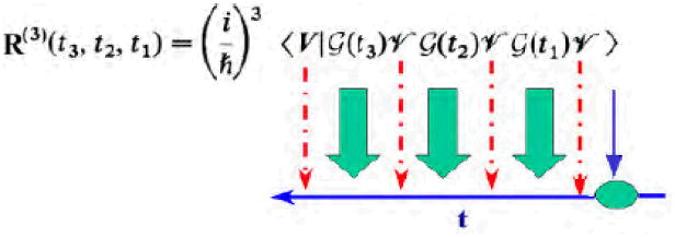
Fig. 8. The schematic representation of third order response function.
Time resolved measurements can monitor the ps- to ns dynamics by following the variation of the cross peaks with time, [112] Hamm had monitored the unfolding of a tetra-peptide triggered by breaking the disulfide bridge between the first and the third residue by a UV pulse [22, 92]. The crosspeaks reveal a few-picosecond timescale hydrogen bonding dynamics. Tokmakoff had reported the steady-state and transient conformational changes in the thermal unfolding of ubiquitin with 2DIR of the amide I vibrations. [113]. Equilibrium measurements are consistent with a simple two-state unfolding, the transient experiments show a complex relaxation pattern that varies with the spectral component and spans 6 decades in time. Using time-resolved IR spectroscopy, Hamm had reported strongly temperature-dependent non-exponential spectral kinetics of the folding and unfolding of a photoswitchable 16-residue alanine-based alpha-helical peptide from few picoseconds to almost 40 1s over the temperature range 279-318 K [114]. Both processes show a complex, indicated an observed stretched-exponential responsebroad distribution of rates was needed to explain. Environment effects on the vibrational dynamics of tungsten hexacarbonyl in cryogenic matrices were investigated using an infrared free-electron laser by measuring the population relaxation time T1 in pump-probe and the dephasing time T2 in a two-pulse photon-echo.[115] Fast (less than a few ps) enzyme dynamics at the active site of formate dehydrogenase (FDH) in complex with azide (N3, a nanomolar inhibitor, and a transition state analogue) and nicotinamide (NAD+) were observed by infrared photon echo measurements. These studies show that the active site of the reactive enzyme complex near the catalytic transition state exhibits the fast dynamics required to explain the kinetics of several enzymes. [116]. Harris and coauthors showed that 2D-IR spectroscopy can provide direct information about the transition-state geometry, time scale and reaction mechanisms by tracking the transformation of vibrational modes as Fe-(CO)5 crossed a transition state of the fluxional rearrangement.[117]. Ultrafast IR-Raman spectroscopy (mid IR pump and Raman probe) were applied to study fast energy transfer dynamics in liquid water, HOD in D2O, and methanol[118, 119].
The hydrogen bonding structure and dynamics in liquid water have been
extensively studied by 2DIR. TokmakoR had investigated rearrangements of the
hydrogen-bond network by measuring fluctuations in the OH-stretching frequency of
HOD in liquid D2O. The frequency fluctuations were related to
intermolecular dynamics. The model reveals that OH frequency shifts arise from
changes in the electric field acting on the proton. At short times, vibrational
dephasing reflects an underdamped oscillation of the hydrogen bond with a period of
170 femtoseconds. At longer times, vibrational correlations decay on a
1.2-picosecond time scale due to collective structural reorganizations
[120]. In 2005, a
combined femtosecond 2D IR and molecular dynamics simulations study focused on the
stability of non-hydrogen bonded species in an isotopically dilute mixture of HOD in
D2O-hydrogen-bonded configurations and non hydrogen bonded
configurations were shown to undergo qualitatively different relaxation dynamics
[121].Water dynamics has
been widely studied theoretically. Molecular dynamics electronic structure
calculations were used to obtain the time correlation functions (TCF) for two water
force fields, TIP4P and SPC/E [122]. The TCFs are inputs to time-dependent theoretical 2DIR
spectra. Comparison with experiment demonstrates that both models overemphasize the
fast (300  400 fs) fluctuations and do
not account for the slowest fluctuations (1.8 ps). The time dependence of the
vibrational echo correlation spectra provides a good test for the TCF. Temperature
dependence of the OH stretch photon echo signal of liquid H2O showed that the
frequency (thus structural) correlations decrease from 50 fs to 200 fs as
temperature decreases from 297 to 274 K, which suggested the reduction in dephasing
by librational excitations. [123].Simple anions (CN−, ) have been used as probes of the fluctuations of
water H-bonding networks[124-126].
400 fs) fluctuations and do
not account for the slowest fluctuations (1.8 ps). The time dependence of the
vibrational echo correlation spectra provides a good test for the TCF. Temperature
dependence of the OH stretch photon echo signal of liquid H2O showed that the
frequency (thus structural) correlations decrease from 50 fs to 200 fs as
temperature decreases from 297 to 274 K, which suggested the reduction in dephasing
by librational excitations. [123].Simple anions (CN−, ) have been used as probes of the fluctuations of
water H-bonding networks[124-126].
Electrostatic interactions are crucial for enzyme activity and drug design. Non-covalent electrostatic couplings of co-factors are sufficiently weak to allow for reversible binding. [127, 128]. 2DIR should provide a direct means for monitoring the electrostatic environment and its fluctuations. Artificial chromophores such as nitriles could be inserted in specific sites in the active region [129]. A 2DIR study of a HIV drug complex containing two nitrile groups [130] shows spectral splitting attributed to the binding environment. Several bond types, including nitriles, carbonyls, carbon-fluorine, carbon-deuterium, azide, and nitro bonds were used as probes for electric fields in proteins using Vibrational Stark spectroscopy. The measured Stark shifts, peak positions, and extinction coefficients may be used to design amino acid analogues or labels to act as probes of local environments in proteins. [131] Vibrational energy transfer pathways [132] may be followed by 2D techniques [118, 133]. Vibrational energy relaxation were simulated by employing the semiclassical approximation of quantum mechanical force-force correlation functions [134].
2D techniques may also be used to retrieve useful information on reaction rates, mechanisms and yields. Small peptides at thermal equilibrium in solution rapidly (within 10∼100 ps) hop among different configurations. The dynamics of these transient species can influence the folding. Hochstrasser [135] and Fayer [136] had independently carried out a 2DIR analogue of chemical exchange for the investigation of ultrafast Hydrogen bonding dynamics of solute/solvent complexes. Hamm had employed nonequilibrium 2D-IR exchange spectroscopy to map light-triggered protein ligand migration [137].
The bond connectivity patterns in molecules have been measured by relaxation assisted 2DIR signals by focusing on two parameters, a characteristic intermode energy transport arrival time and a cross-peak amplification coefficient. 2DIR spectra of the coupled carbonyl stretches of Rh(CO)2(C5H7O2) in hexane have been obtained from femtosecond vibrational echo signals detected with spectral interferometry. This experiment characterizes the structure with a time window of roughly 20 ps [138].
III. An Effective Fluctuating Exciton Hamiltonian for the Amide Vibrations of Polypeptides
Vibrational spectra are commonly described by normal modes, which represent the collective motions of the atoms when all anharmonicities are neglected. The normal mode frequencies and individual atom displacements may be calculated from molecular mechanics force fields implemented in standard MD codes. These are parameterized to represent slow backbone motions. High-frequency vibrations such as the amide bands of peptides require more expensive ab-initio calculations.
A peptide can be viewed as a chain of beads connected by amide bonds (O=C-N-H) (Fig. 3). These have a partial double-bond character and due to steric effects are almost exclusively in the trans configuration. The area between two consecutive α-carbons (peptide unit) is thus rigid and planar. The peptide backbone structure is described by two dihedral Ramachandran angles A and A per amide bond. The infrared spectrum of the backbone peptide bonds consists of four amide vibrational bands, known as the amide I, II, III and A [139, 141]. These amide bands originate from the coupled localized amide vibrations on each peptide unit (local amide modes (LAMs)) The localization may be visualized by expanding the molecular charge density .(r) in nuclear displacements:
Fig. 3.

The amide bonds and Ramachandran angles (ϕ and Ψ). The planes marked by green lines are peptide units. “Sc” represent side chains.
| (1) |
where qmi is the i′th vibrational mode of the n′th peptide bond. The transition charge density (TCD) ∂p / ∂qmi [142] represents the electronic structure change induced by the qmi vibration. The 0.01 esu/Bohr (TCD) contours of the 4 amide vibration of N-methyl acetamide (NMA), a model system of the amide bond, are shown in Fig. 4. The amide III(∼1200 cm−1), II(∼1500 cm−1) modes are attributed to bending motion of the N-H coupled to C-N stretching. The 1600-1700 cm−1 amide I mode originates from the stretching motion of the C=O stretch coupled to in-phase N-H bending and C-H stretching. The amide A (∼3500 cm−1) is almost purely the N-H bond stretch. [139, 140, 143]. All TCD are highly localized on the 4 atoms (O, C, N, and H) forming the amide bond. The overlap of the amide excitations between different amide bonds is small and is limited to nearest neighbor amide III amide II amide I amide A peptide bonds. By parameterizing the Hamiltonian and transition dipole elements of all amide bands (I, II, III and A) by the Ramachandran angles, we can avoid the repeated electronic structure normal mode calculations for various conformations.
Fig. 4.

Transition charge densities (TCD) for the 4 amide modes of NMA. Shown is the 0.01 esu/Bohr contour. Violet and brown contours represent positive and negative values, respectively.
The sensitivity of the amide vibrational transitions to the local structure and hydrogen bonding environment makes them ideal candidates for distinguishing between various secondary structural motifs and monitoring eRects of the changing environments [144]. The intense and spectrally-isolated amid I band is particularly suitable for structure determination. Its frequency variation with the secondary structure and conformation is widely used as a marker in polypeptide and protein structure determination [56, 57, 105, 143-146]. α – helical peptides have amide I bands between 1650 - 1655 cm−1. β – sheets usually have a strong band between 1612 - 1640 cm−1 and a weaker ∼1685 cm−1 band. Random structures generally have a 1645 cm−1 band, which is close to the frequencies associated with α – helix. There are three other distinct amide infrared bands. The antiparallel β – sheet structure shows a strong amide II band between 1510 and 1530 cm−1, whereas a parallel β – sheet structure has higher frequency (1530-1550 cm−1). Deuterium substitution results in substantial shift to lower frequency (∼1460 cm−1). The amide III infrared band is typically weaker than the amide I and II. Deuteration also shifts the amide III band to lower frequencies (960 - 1000 cm−1). This band is usually not correlated with protein secondary structure, but is sensitive to hydrogen bonding and local Ramachandran angles[19]. The amide III band is sometimes used in combination with the amide I band to distinguish the β – sheet and disordered structure which is not generally possible with only the amide I band. The overlap of the amide A with the intense O-H band of water complicates its observation and interpretations.
A Hamiltonian adequate for 2DIR simulations of peptides may be constructed by expanding the potential in LAMs up to 6th order within each peptide unit, to 4th order for neighboring couplings, and to 2nd order for non-neighboinr electrostatic couplings (Eq. (2)) [147, 148]. Interactions between LAMs with non-overlapping TCD are purely electrostatic and are given by:
| (2) |
By diagonalizing the local Hamiltonian for each amide bond without their couplings, we obtained 14 local amide eigenstates (4 fundamentals, 4 overtones, and 6 combinations) in the energy range 0 - 7000 cm−1 for a single peptide unit. We define the exciton creation and annihilation operators for a′th LAS on the m′th unit B̂ma≡|ma〉〈m0| and where |m0〉 is the ground state. These satisfy the Pauli commutation relations: The peptide Hamiltonian is then recast in terms of these operators [148]:
| (3) |
The first term represents the local Hamiltonian, and the second contains couplings between neighboring peptide units. These were computed as a function of the Ramachandran angles (φ and Ψ) at the BPW91/6-31G(d,p) level of DFT using a quartic anharmonic vibrational DFT potential of various glycine dipeptide (GLDP) configurations. The electrostatic model is used for couplings between non-neighboring units (the last two terms in Eq. (3). The transition charge density couplings (TCDC) (Eq. (2) was expanded to 4th rank in multipoles. This results in ∼R−3 (dipole-dipole), ∼R−4 (dipole-quadrupole), ∼R−5 (quadrupole-quadrupole and dipole-octupole) interaction terms where R is the distance between units.
Torii and Tasumi (TT) had constructed the same type of map [146] for the amide I neighboring coupling using restricted Hartree-Fock (RHF) electronic structure calculations of glycine dipeptide (GLDP). The amide I through-space coupling between the non-neighboring peptide units was approximated by the transition dipole coupling model (TDC). [149,150]. The magnitude, direction, and location of the transition moment were fitted to reproduce the ab initio coupling constants between the second nearest amide units (the magnitude of the transition dipole was (∂μ/∂q) = 2.73 D A−1 with 10.0 ° angle to the C=O bond). Gorbunov, Kosov and Stock [151] derived a similar map at higher (MP2 and B3LYP) computational level. Woutersen and Hamm approximated through-space TCDC with Mulliken partial charges of a NMA DFT calculation to include higher multipole contributions for the amide I vibration [152], which was later improved by using multipole derived charges [153]. The accuracy of the amide I local eigen frequencies and infrared intensities with respect to reference DFT calculations was slightly improved (0.1 cm−1 in frequency and 0.02 in infrared intensity correlation) by including higher multipoles (Table V of Ref [153]). The transition multipole couplings extended the transition dipole couplings to include higher multipoles of all amide modes. The higher multipole contributions are more important for amide modes II, III and A than I since the amide II and III are more delocalized over the peptide bond, and the amide A has a smaller transition dipole (Fig. 8 of Ref. [147]). The dipole coupling with the radiation field is
| (4) |
To account for chirality this was extended to include magnetic moments. Derivatives of magnetic moments with respect to the LAM depend on the Ramachandran angles Ψ and φ. The map of magnetic moment derivatives was obtained by DFT calculations of a chiral model peptide unit which has a similar structure to NMA (Fig. 1 of Ref [148]). Magnetic moment derivatives may be calculated based on the atomic axial tensor and the normal modes [154].
Electrostatic Fluctuations of the Local Hamiltonian
The local Hamiltonian (Eq. (3)) depends on the electrostatic environment induced by the surrounding peptide residues and the solvent. The amide I frequencies are shifted to the red by hydrogen bonding with water. Electrostatic modeling of the fluctuating local Hamiltonian requires repeated ab-initio vibrational potential calculations of the peptide bonds surrounded by the partial charges of the surrounding peptide residues and the solvent. Simulation of 2DIR lineshapes in NMA require the construction of a Hamiltonian along the MD trajectory with typically ∼105 snapshots. These repeated ab initio calculations can be avoided by an electrostatic parameterization of the Hamiltonian. The local electrostatic environment may be simply described by an electric field at some reference point [155]. Such linear Stark modeling works for smaller chromophores [120, 156, 157] The nonuniform electric field across the peptide bond should be taken into account [142].
Ham and Cho (HC) had obtained a map which parameterizes the amide I frequencies as a linear function of the electrostatic potentials at the C, O, N and H and two methyl sites [158, 159] by the least square fit of the normal mode frequencies of NMA-water clusters at the Restricted Hartree-Fock (RHF). Schmidt, Corcelli, and Skinner [160] had constructed a similar map (SCS) of the NMAD amide I frequency, where the frequency was parameterized as a linear function of the electric fields at the C,O,N and H atoms, and the electronic structure calculations were made at the DFT level. Watson and Hirst had found that the accuracy of NMA amide I frequencies in water is improved by additional sampling points in the amide bond (mid points of CO,CN, and NH) of electrostatic potentials [161].
We have parameterized the fundamental, the overtone and the combination frequencies and transition dipoles of all amide modes (III, II, I and A) as a quadratic function of the multipole electric field up to 2nd derivatives of the electric field at a midpoint of amide oxygen and hydrogen atoms (HM map) [142]. The map was constructed by repeated eigenstate calculations of the 6th order anharmonic DFT (BPW91/6-31G(d,p)) vibrational potential in 5 relevant normal modes of NMA in the presence of different nonuniform multipole electric field. The fundamental frequencies as well as anharmonicities are parameterized, and geometry changes and mode mixing induced by the multipole electric field are included. The average and the correlations between the fundamental and anharmonicity frequency fluctuations determine the relative positions and intensities of two positive (stimulated emission/ground state bleach) and negative (excited state absorption) peaks of the nonlinear infrared signals [162] Unlike the maps of Cho and Skinner, this map does not involve a fitting to a specific solvent. A similar approach was later adopted for the amide I frequency by Jansen and Knoester [163] who constructed the amide I single mode anharmonic vibrational potentials for NMA embedded in a set of different solvent charge distributions. The amide I frequencies were parameterized by the electric field and gradients at the C, O, N and H atoms. The map does not include mode mixing. Frequencies and infrared intensities of a pentapeptide in several gas phase configurations [161] calculated by this map combined with transition charge couplings and neighboring coupling map were in good agreement with DFT calculations [153]. Cho's map had a similar agreement.
The Torii and Tasumi couplings were used with our local Hamiltonian in earlier applications [164]. The full Hamiltonian (Eq. (3)) was employed for two α helical peptides (SPE3 [145]) reported later in this section.
The segment made of a given amide residue and two neighboring neutral groups of the CHARMM27 force field [165] was used as the basic chromophores in the electrostatic interaction calculations(Fig 3). The effect of the rest of the protein and the solvent is described by a fluctuating electrostatic flield. The electrostatic potential U is expanded to cubic order in local Cartesian coordinates Xα. (α ; β = x, y, z) around the midpoint between amide oxygen and hydrogen atoms of the amide bond (Fig. 5),
Fig. 5.

Left: NMA molecular structure and coordinate system used for the anharmonic force field and the electrostatic potential. The four amide atoms (O4, C3, N2, and H6) are in the x-y plane. The origin is the middle point of the oxygen (O4) and hydrogen (H6). Right panels: Contour plots of the nonuniform electric field (Ex and Ey) of NMA in H2O. Red circles represent the four amide atoms (O4, C3, N2, and H6). The sampling points are shown by the blue crosses.
| (5) |
Apart from the trivial reference U0, Eq. (5) has 19 independent parameters arranged in a vector C = (Ex,Ey,Ez,Exx,Eyy,Ezz,Exy,Exz,Eyz,Exxx,Eyyy,Ezzz,Exyy,Exxy,Exxz,Exzz,Eyzz,Eyyz,Exyz) (note the symmetry Eαβ = Eβα).
The components of C are determined at each time step by a least-square fit to the electric field sampled at 67 points in space spanning the TCD region of the 4 amide modes (Fig. 5). We expect the electrostatic potential in the region of large TCD to affect the infrared activity of that vibration. Four sampling points at C,O,N and H atom positions were not sufficient to predict the solvent frequency shits (especially the amide II and III) [142]. This is consistent with the result by Watson and Hirst where increasing sampling points improved the amide I frequency shit accuracy [161]. The parametric dependence of the anharmonic force field on the electrostatic multipole coefficients C was obtained for NMA [142] at the BPW91/6-31G(d,p) level [166]. This functional is known to give accurate amide vibrational normal mode frequencies of peptides[167]. Analytic energy gradient in the presence of multipole field was implemented in the Gaussian 03 code [168] to compute the higher derivatives [169, 170].
The LAS were calculated for a grid of electrostatic multipole coefficients C by diagonalizing the local Hamiltonian expanded in a harmonic basis set. The ARNOLDI matrix diagonalization algorithm was employed in these vibrational configuration-interactions (vibrational CI) calculations. The vibrational transition frequency from the ground state to LAS a and the transition dipole moments between LAS a and Insert equations 6 and 7 b at the m0th peptide unit were expanded to quadratic order in C:
| (6) |
| (7) |
where the gas phase frequencies were taken from experiment [171] and Oα(1) a and M(1)ab are 19 component vectors representing the first derivative of the frequency and the transition dipole with respect to the C. O(2)a and Mα (2)ab are the second derivative 19×19 matrices.
To trace the origin of the electrostatic effects on the amide frequency shifts, the C=O and N-H bond lengths obtained by energy minimization for the various field values were parameterized in terms of C[142]. Strong correlations are seen in the scatter plots of the 4 amide fundamental frequencies with C=O and N-H bond length displayed in Fig. 6. These suggest that structural changes of NMA caused by the electric field [142, 146, 155, 172, 173] are responsible for the frequency shifts. The positive correlations of the two bending frequencies with the N-H bond length are ascribed to the fact that the hydrogen bonding to H6 causes a longer N-H bond length and makes the potential more stiff along the amide II and III bending modes by stabilizing the parallel N2-H6….OH2 structure.
Fig. 6.

Scatter plots of amide frequencies versus bond lengths. Linear fits are ω = 6549:2 - 3905RCO (amide I vs C=O bond length), ω = 24259- 20426RNH (amide A vs N-H bond length), ω = -3066 + 4278RNH (amide III vs N-H bond length) and ω = 2768 + 4204RNH (amide II vs N-H bond length). The gas phase values are marked by green cross.
The simulated amide I solvent peak shifts (−59 cm−1) and line widths (29 cm−1) of NMA in water are in good agreement with experiment (−80 cm−1 and 29 cm−1 respectively). This effective Hamiltonian was applied to SPE3, a 16 residue α –helical peptide (YGSPEAAA(KAAAA)3r, r represent D-Arg) [145]. The fluctuating Hamiltonian was constructed for 100 snapshots obtained from a 2 ns MD trajectory [164]. The vibrational eigenstates were calculated by diagonalizing the HM Hamiltonian. A good measure of the coherence length Lν of the ν′th vibrational eigenstate is provided by the participation ratio [54, 65, 174]:
| (8) |
where Cv,ma is the expansion coefficient of the ν′th eigenvector on LAS a at the n′th th peptide unit. The distributions of Lo binned over frequencies of the eigenstates in 4 amide fundamental regions are shown in Fig. 7. In the amide I region, the lower frequency eigenstates (∼1600cm−1) are mostly localized on one amide bond (<Lv> ≪ 1), the higher frequency eigenstates are delocalized. The higher frequency amide III eigenstates (∼1300 cm−1) are localized. In the amide II region, there are two or three peaks in participation ratio distribution. The amide II fundamentals are the most delocalized with <Lν> = 2.3, due to the larger neighboring couplings and transition moments, and smaller diagonal frequency fluctuations. The amide III and I fundamentals are delocalized over 1.6 and 1.8 amide bonds. The amide A modes are highly localized (hLoi = 1:0) due to the small transition moment and large frequency fluctuations. This localization is good news for the interpretation of 2DIR signals in terms of local structure.
Fig. 7.

Distribution of the participation ratio (PR) vs frequency in the amide III, II, I and A regions. Average PRs are 1.6 (amide III), 2.3 (Amide II), 1.8 (amide I), and 1.0 (amide A), respectively.
IV. Liouville-Space Pathways for the Optical Response of Coupled Localized Vibrations
Coherent optical signals can be classified by their power-law dependence on the driving field intensities [66]. The signals are related to the polarization, P(t), induced by the external electric fields. The induced-polarization can be obtained perturbatively by expanding density matrix ρ(t) in powers of the external fields [66]. The third order response function, represents the lowest order contribution to the induced polarization in isotropic systems:
| (9) |
where r and t1, t2, t3 represent the coordinates and the interaction time intervals between successive interactions with the optical pulses, E(r, t) (see Fig. 1). ν j are the Cartesian components of the fields and polarizations. The response functions are system property-tensors that contain all relevant molecular information. R(1) is a second-rank tensor connecting two vectors (E and P). Similarly, R(3) is a fourth-rank tensor. A heterodyne-detected four wave mixing experiment (Fig. 1) [175] involves four pulses. In ideal impulsive measurements the pulses are temporally ordered, well separated, and much shorter than the relevant molecular timescales. Under these conditions, all integrations in Eq. 9 can be eliminated and the optical signal is simply proportional to the response function itself. The third order response is illustrated in Fig. 8. The system is initially in thermal equilibrium, and the Green's function G(tn) describes the free molecular time evolution (without the fields). At time 0 it interacts with the first pulse (Vν1), propagates freely during t1 (G(t1)), interacts with second pulse (ν̂ν2) at t1, propagates during time t2 (G(t2)),interacts with third pulse (ν̂ν3) at t1 + t2, propagates during t3 (G(t3)), and finally interacts with the signal mode (ν̂ν4) at t1+t2+t3 to create the response. The dipole operator can act three times either on the ket or the bra.
The third order response function is thus given by a sum of 23 = 8 four-point correlation functions [66] which constitute the 8 basic Liouville space pathways:
| (10) |
Different techniques can select some of the possible terms in Fig. (8), depending on the pulse configuration and the detection mode. To compute the signals, the electric field E 25 must be expanded in modes:
| (11) |
where pulse j = 1, 2, 3, s is centered at τj, with wavevector kj, carrier frequency ωj, phase ωj and complex envelope ενj(t−τj). We shall label the three incoming pulses and the signal as 1,2,3 and s. The k1 pulse comes first, followed sequentially by k2, k3 and ks. The heterodyne-signal S(t), defined as the change in the transmitted intensity of mode s induced by the other three beams, is the convolution of P(3), the third order polarization, and the external fields.
| (12) |
where the r integration runs over the interaction volume in the sample.
Coherent nonlinear signals are highly directional and are only generated when ks lies along one of the following phase-matching directions: ks = ±k3± k2±k1 (with the corresponding frequencies ωs = ±ω3 ±ω2 ±ω1). This important feature of coherent spectroscopy stems from the fact that we add the field amplitudes generated by different molecules and that the sample is much larger than the optical wavelength [296]. Random phases then cancel the signals in other directions. Incoherent signals, such as fluorescence are obtained by adding the intensities (amplitude squares), and the signals are essentially isotropic. A whole host of names and acronyms have been used for various combinations of vectors and time intervals (e.g. photon echo, transient grating, CARS, HORSES, etc). NMR has it own set of acronyms (COSI, NOE…) We shall avoid this nomenclature and simply classify the signals into four basic techniques: kI = −k1 + k2 + k3, kII = k1 −k2 + k3, kIII = k1 + k2 + k3 and kIV = k1 + k2 + k3.
The dominant contributions to resonant signals only come from terms obtained when the field and molecular frequencies in Eq. 9 have an opposite sign. Other (same-sign) highly- oscillatory terms may be safely neglected. Using this rotating wave approximation (RWA), each phase-matching signal is described by a specific combination of Liouville space pathways. For the kI technique we have:
| (13) |
The dependence of R(3) ks,ν 4ν 3ν 2ν1 (t3, t2, t1). on the wavevector comes by selecting the RWA pathways.
To invoke the RWA we must specify the model. The amide band energy level scheme consists of three well-separated bands as shown in Fig. 9. Only transitions between the ground state, g, and the first excited states manifold, e, and between the first and second excited state manifold, f, are allowed. The response functions may be calculated by summing over all possible transitions among vibrational eigenstates. The nonlinear response vanishes for harmonic vibrations and may thus be attributed to the anharmonicities. The exciton Hamiltonian introduced in Sec. III represents a multilevel system. Each amide unit can be modeled as a 3 level system. The global eigenstates of the entire peptide then consist of the ground state |g >, a single exciton band |e > and a double exciton band |f >. The level-scheme is given in Fig. 9.The terms that contribute to the signal can be represented using Feynman diagrams which represent the evolution of the density matrix and are constructed with the following rules:
Fig. 9.

Energy level scheme for the systems considered. g is the ground state, e is the first excited state manifold and f is the second excited state manifold. The transitions that can be induce by the pulses are shown as μge and μef.
The density matrix is represented by two vertical-lines. The line on the left represents the ket and the line on the right represents the bra.
Time runs vertically from bottom to top.
Each interaction with the radiation field is represented by a wavy-line. An arrow pointing to the right and labeled kj represents a contribution of εj exp(−iωjt + ikj.r) to the polarization. An arrow pointing to the left represents a contribution of .
Each diagram has an overall sign of (−1)n where n is the number of interactions from the right (bra) (an interaction ν̂ that acts from the right in a commutator in the Liouville equation carries a minus sign). The Feynman diagrams for the kI technique are depicted in Fig. 9. They show the state of the density matrix during each time interval. Computing the signals generally involves multiple integrations over the pulse envelopes (eq. 9). Obviously, the shape and relative phases of the pulses are important factors which affect the signal. Coherent Control and pulse shaping algorithms may be used to design signals that meet desired targets [64]. We shall focus on ideal time-domain techniques where the pulses are well separated temporally. Multi-dimensional signals are displayed in the frequency-domain by performing the multiple Fourier transform of S(3) ks (t3, t2, t1) with respect to the time intervals between the pulses. We shall consider the following signal:
| (14) |
This signal is given by [176].
| (15) |
| (16) |
| (17) |
These expressions show how the pulse envelopes select the transitions lying within the pulse bandwidths. e and e′ run over the first excited state manifold and f includes the second excited states manifold (Fig. 9). ω1, ω2 and ω3 are the carrier frequencies of the first three pulses. ωab = (εa − εb)/ħ are the transition frequencies where the ε's are the state energies and ξab = ωab − iγab are complex transition frequencies which include the dephasing rates γ in the impulsive (broad bandwidth) limit we simply set ε(ω) = 1.
A. Simulating 2DIR of Small Peptides; Gaussian Frequency Fluctuations
We now turn to a special class of fluctuation models [55, 62] which may be solved exactly, yielding compact closed-form of expressions for the response functions. These have been successfully applies for modeling 2DIR signals of small peptides with less than 30 residues.
We assume purely diagonal (energy) fluctuations with Gaussian statistics. The fluctuations are small compared to level spacings. This is the case when the energies are modulated by collective coordinates expressed as sums of harmonic coordinates. However, the model may hold more broadly, thanks to the central limit theorem, when the collective coordinates are given by sums of many bath coordinates, each making a small contribution. One notable example is when the collective coordinate is the electric field at a given site, given by the sum of contributions from all charges in the solvent. This is the basis of Marcus theory of electron transfer [177]. We shall make the Condon approximation and neglect fluctuations of the transition dipole magnitude.
The response functions can be calculated using the second order Cumulant expansion which is exact for this model (denoted as CGF: Cumulant expansion of Gaussian fluctuations). To that end, we introduce Uma(t) ≡ ωma(t)−ω̄ma representing the fluctuations of the transition frequencies, where ω̄αβ is the average transition frequency. The two-time correlation function of U is:
| (18) |
where C′(t) and C″(t) are the real and imaginary parts of C and τ12 = τ1 − τ2. We further define the line-broadening functions:
| (19) |
using the fluctuation dissipation relation between C′ and C″ gmn(t) can be expressed as
| (20) |
Where
| (21) |
is known as the spectral density. The real and the imaginary parts of gnm(t) are responsible for line-broadening and shift, respectively. The third-order nonlinear response functions can be expressed in terms of g(t) [66]. This will be denoted as CGF (Cumulant expansion of Gaussian fluctuations).
Simulated kI and kIII signals of all amide modes of NMA in water in the cross peaks regions are shown in Fig. 11. The simulations reproduce the amide I and II anharmonicities obtained by the recent cross peak experiment (calc: 14 cm−1 and 13 cm−1; exp: 12 cm−1 and 10 cm−1, respectively).
Fig. 11.
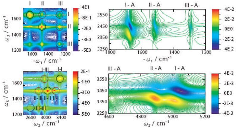
2D signals of a model system for the peptide bond (NMA) in the cross peak region of amide I, II and III and A modes. Top panel left: Im[SkI (− Ω1, t2 =0, Ω3) in the cross peak region of amide I, II, and III modes; bottom left panel: Im[SkIII(t1 = 0, Ω2, Ω3) ] in the cross peak region of amide I, II, and III modes. Right panels show the same signals in the cross peak regions of the amide A and amide I, II and III modes.
The frequency-frequency correlation function of two vibrational transitions (Eq.(18)) can be represented as:
| (22) |
where is a fluctuation amplitude,
C̄mn is a normalized correlation
function (C̄mn(0) = 1), and
 mn is the correlation coefficient which varies
between 1 (full correlation), 0 (no correlation), and −1
(anti-correlation).
mn is the correlation coefficient which varies
between 1 (full correlation), 0 (no correlation), and −1
(anti-correlation).
To investigate the sensitivity of coherent infrared signals to correlated frequency fluctuations, we present the amide I - III photon echo cross peak of NMA (Im[ SkI (Ω1, t2 = 0, Ω3) ]) in Figure 12 for various combinations of the correlations coefficients. Negative and positive peaks of the kI signal correspond to the ESA and ESE/GSB pathways of Fig. 10 respectively. Correlations between the amide I and III (η13) contribute to the negative components and correlation between the amide III and the combination state I+III(η19) contributes to the positive component. The negative peak becomes weaker and broader as η13 is varied from +1 to −1, but does not depend significantly on η19. The positive peak becomes smaller and broader elongated more in Ω3 direction as η19 goes from full correlation (+1) to anti-correlation (−1). The actual simulated values (anti-correlated η1,3 0.71 and correlated η1,9 = 0.63) gives weaker signals than when both are fully correlated.
Fig. 12.

The amide I - III kI cross-peak signals of NMA for different correlation coefficients. Left panels: Im ∣ SkI (Ω1, t2 = 0, Ω3)∣ signal for different η1,3 and η1,9 ; right panels: the actual simulated signals.
Fig. 10.

Double-sided Feynman diagrams representing the Liouville space pathways contributing to the kI signal in the rotating wave approximation. The three pathways are known as excited state emission (ESE), the ground state bleaching (GSB), and excited state absorption (ESA), as indicated.
For systems with several local minima whose dynamics can be separated into well-separated time regimes, we can adopt the inhomogeneous CGF protocol [76]. The spectrum is obtained by summing over contributions of the slowly interconverting configurations, each represented by the CGF. This protocol is illustrated for the 1D and 2D IR spectra of a specific tryptophan zipper peptide, trpzip2 in a β -hairpin conformation and its 13C isotopomers in the amide-I region. β -hairpins are common protein structural elements which provide an important model system into the folding kinetics of larger proteins. Their structure and folding dynamics have been studied extensively. One structural motif, the tryptophan zipper (trpzip), greatly stabilizes the beta -hairpin conformation in short peptides(12 or 16 Å in length). Trpzips are the smallest peptides to adopt a unique tertiary fold without requiring metal binding, unusual amino acids, or disulfide crosslinks. 500 snapshots with 2 ps time intervals were selected from the 1 ns trajectory and used for the inhomogeneous averaging. A 5.5 cm−1 homogeneous dephasing rate [178] γ was added. Two electrostatic maps (HC [158] and HM [142] as described in Sec.II) were used to compute the solution-phase local mode frequencies in solution. Spectral features for the sample with no isotope labeling (UL), and with the 13C isotope labeled at specific residues are calculated. The sample with a β strand residue (the second residue) labeled is denoted L2, while the sample with a turn residue (the seventh) labeled is denoted L7. The simulated signals are compared with experiment in Fig-13 and Fig-14.
Fig. 13.

IR spectra of trpzip2 13C isotopomers Solid lines: UL; dashed lines: L2; dotted lines: L7. (A)Experimental and simulated using HC electrostatic potential model [158] (B) and the HM multipole field model [142] (C).
Fig. 14.

(A-C) Experimental kI +kII spectra of trpzip2 13C isotopomers. (D-F) simulations using the HC Hamiltonian [158]; (G-I) simulations results using the HM Hamiltonian [142]. Left column is for UL, middle for L2 while right for L7. ωτ is Ω1 in the notation of this review, while ωτ is Ω3.
The experimental absorption spectra of trpzip2 13C isotopomers in the amide-I region are displayed in Fig.13 show two main transitions: the stronger low frequency, ∼1640 cm−1, transition is due to inter-chain in-phase and intra-chain out-of-phase C=O motions, whereas the weaker high-frequency ∼1675 cm−1, transition is mainly due to the inter-chain out-of-phase and intra-chain in-phase C=O motions. The two isotopomers show different 13C effects: the 13C band is shifted 10 cm−1 to the red in L7 than in L2 (1590 vs. 1600 cm−1). Simulated spectra are shown in panel (B) (HC Hamiltonian) and (C) (HM Hamiltonian). The high frequency component is slightly stronger for the HM, but overall both models reproduce the main spectral feature of the unlabeled β -hairpin. In addition, both predict a small difference in the observed 13 C-shifts between L2 and L7. The difference is slightly larger in the HM simulation.
The top row in Fig. 14 shows the experimental kI + kII spectra of the trpzip2 13C isotopomers. In panel (A), the diagonal signals are due to 0-1 (red) and 1-2 transitions (Blue). The two fundamental 0-1 frequencies agree with the experimental absorption, as can be seen by projecting the 2D spectrum onto the Ω3-axis. The cross peaks are induced by pairwise vibrational couplings among local amide-I modes. The diagonal and off-diagonal peaks, change upon 13C-labeling as shown in panel (B) and (C). The spectra simulated using the HC model are shown in the middle row and the HM simulations (bottom row). The main 2D IR characteristics of the UL, L2, and L7 are reasonably reproduced by both models.
The effect of the multiple state nonadiabatic crossing between amide I vibrational energy surfaces was recently investigated [179].
V. Spectral-Diffusion and Chemical-Exchange; The Stochastic Liouville Equations (SLE)
The Cumulant expressions used in the previous section provide a simple compact description of bath fluctuations with Gaussian statistics coupled linearly to the frequencies. More general fluctuations require a more elegant treatment. We need to work in an expanded phase-space that includes relevant collective bath modes and compute the evolution of distributions in this extended space. The Stochastic Liouville equations (SLE) proposed by Kubo [180-183] to represent the dynamics of the distribution of a quantum system perturbed by a stochastic process described by a Markovian master equation. The SLE are widely used in the simulations of electron spin resonance (ESR)[184,185], NMR [183] and infrared [186,187] lineshapes.
Below we demonstrate its power by simulating 2DIR spectra of a small peptide, trialanine, and chemical exchange processes [188]. Trialanine has two amide bonds which contribute to its amide I band. The Hamiltonian depends on the frequencies ωa and ωb, anharmonicities Ka and Kb and the coupling constant J of the two local modes. The simulations presented below include 6 vibrational energy levels: the ground state (g), two single excited levels (e1 and e2) and three doubly excited levels (f1, f2 and f3) (Fig. 9). The time evolution of the density matrix describing the state of the two mode system is described by the Liouville equation
| (23) |
represents the isolated system, while represents the coupling with the radiation field.
Analysis of the amide I absorption band of trialanine. [100, 189-191] suggests that it primarily exists in the polyglycine II (PII) structure (a conformation characterized by Ramachandran-angles of (Ψ, φ) = (−60°, + 140°) and a right hand R helix (α R) (Ψ, φ) = (−60°,−45°) [192]. We found 70% PII configuration and 30% α R in the joint distribution of the Ramachandran angles derived by the MD trajectory. The Ramachandran angle distribution functions for each configuration were fitted to a Gaussian form. The two configurations are stable and only 38 transitions occurred during the 10 ns simulation, suggesting a few hundred picosecond exchange time of the two species, which is too slow to affect the lineshapes. The response was thus calculated as an inhomogeneous average over the two species. The nonadiabatic effect of the two state curve crossings has been also investigated [179].
The frequency fluctuations of the two modes (δωa) and (δωb) are treated as independent stochastic variables. These are dominated by the interaction with the solvent water molecules in the vicinity of each amide unit. The Brownian oscillator parameters (relaxation times γa −1 = γb −1 = 220 fs and magnitudes Δa = Δb = 16.1 cm−1 reproduce the experimental lineshape for the isolated amide I mode in NMA. [159] The fundamental frequencies are given by ωa =< ωa > +δωa and ωb =< ωb > +δωb with average frequencies < ωa >= 1652 and < ωb > = 1668 cm−1. [189, 190] The difference stems from the charge on the terminal amino group; the amide unit closest to the acid group has the lower frequency.
Ramachandran-angle fluctuations (δφ and δΨ) constitute another set of relevant stochastic variables that primarily affect the intermode coupling J. J was expanded to quadratic order:
| (24) |
C ij were obtained by a fit to the TT map which connects the coupling constant and the Ramachandran angles[146]. C00 represents the coupling at the average Ramachandran angles which is the reference point for the Taylor expansion. We found C00 = 4 cm−1 in the PII configuration and 10.5 cm−1 for α R.
All four stochastic variables (δωa, δωb, δφ and δΨ) are treated as Brownian-oscillators, each characterized by two parameters Δ (variance of fluctuations) and γ (relaxation rate). The local anharmonicities defined as the differences between the twice of the fundamentals and the overtone frequencies. were fixed to 16cm neglecting their fluctuations. [53, 98, 193] Transition dipole fluctuations of the local modes were neglected as well and their magnitude were set to unity.
The probability distributions P(Q, t) of our stochastic variables Q1 = δωa, Q2 = δωb, Q3 = δφ and Q4 = Q4 = δΨ, is modeled by the Markovian master equation
| (25) |
where Γ(Q) has the Smoluchowski (overdamped Brownian Oscillator)form
The SLE is finally constructed by combining the Liouville equation for the exciton system (Eq. (23)) and the Markovian master equation (Eq. (25)) for the four collective Brownian oscillator coordinates.
| (26) |
The SLE may be solved using a Matrix Continued-Fraction representation of the Green's functions, [188] in the frequency domain. The 2DIR PE signal SkI(Ω1, t2, Ω3)), was computed by transforming the frequency Ω2 back to the time domain.
| (27) |
The Green's function for the t2 interval may also be computed in the time domain by a direct time integration of the SLE. Different levels of simulation of theSIZZZZ signal were compared in Ref-[194]. The highest level (i), includes fluctuations of all four collective bath coordinates. The Liouville operator is constructed in the local basis and the coupling between the two local modes fluctuates with the Ramachandran angles. The local-mode frequencies fluctuate as well. Satisfactory agreement with experiment is obtained as shown in Fig-15. Some differences arise since the RR population is overestimated by the molecular dynamics simulation. Stock et al. [195] had demonstrated that different molecular dynamics force fields predict very different populations of the various conformations of trialanine. In addition, the Ramachandran angles obtained from the MD trajectories. However, the SLE need not necessarily rely on MD simulations and can use e.g. parameters obtained from NMR. In summary, four collective coordinates can account for the effect of fluctuations on the two amide I mods for trialanine. Ramachandran angle fluctuations have significant signatures on 2DIR lineshapes in non-rigid peptides.
Fig. 15.

Top: The experimental kI photon echo spectrum of trialanine [194](left) and the simulated spectrum(right) for parallel polarized pulses. Bottom: Same comparison but for perpendicular polarized pulses. The spectra are normalized to the most intense peak.
The exchange between conformers in trialanine is slow and the signal is given by a sum of the contributions of the various conformers. Fast-exchange shows interesting signatures in 2D signals as demonstrated in hydrogen-bonding and isomerization dynamics [196]. These can be described by including a multi-state jump model in the SLE. The Brownian-oscillator motion and the exchange process show different 2DIR signatures. In the following simulations we allowed a different width for the u and d peaks. The splittings 2Δ0 = 34cm−1(i.e. ∼ 1.01 ps−1) and the exchange rates ku = 0.1ps−1 kd = 0.125ps−1 were taken from the crosspeaks growth of [136]. All three regimes were observed experimentally (the formation and dissociation of phenole-benzene complexes in CCl4 solution) [136]. In the intermediate 2ps timescale regime, memory of the Brownian oscillator coordinate is lost as evident by the circular lineshape but the cross peaks are weak, We thus assumed . Λ ∼ 0.4ps−1 relaxation rate. Λ, Ω1 and Ω3 can be estimated from the absorption linewidth using the Pade approximate of a 2-level system [66]. Simulations reproduced the experimental absorption spectra using Ω2 = 0.33ps−1, Ω3 = −0.07ps−1 . The 2DIR-PE signals shown in Fig 16 recovers all experimental features; all three regimes are clearly seen (a) rephasing elliptic shapes, (b) the relaxed Brownian oscillator with circular shape and (c) chemical exchange cross-peaks as found experimentally (the lower frequency peak is weaker but broader [136]).
Fig. 16.

Simulated 2DIR signals SA = kI + kII for exchange Ω1 = 0.5 fs−1 Λ = 0.4ps−1 ;Ω2 = 0.33ps−3, Ω3 = −0.07ps−1kd = 0.125ps−1,ku = 0.1ps−1, Δ0 = −2.0ps−1,Δ3 = Δ1 = 0. Various time delays (a) t2 = 0; (b) t2 = 2ps; (c) t2 = 10ps. These spectra closely resemble the experimental results of Ref [136].
Various time delays (a) t2 = 0; (b) t2 = 2ps; (c) t2 = 10ps. These spectra closely resemble the experimental results of Ref [136].
The SLE can be used to describe many types of fluctuations of all elements of the Hamiltonian. The only requirement is that they may be represented by a few collective (discrete or continuous) coordinates which satisfy a Markovian equation of motion. These equations account for the effect of the fluctuations of collective bath coordinates on the nonlinear infrared spectra by describing the evolution in the joint system + bath space.
VI. The Oh Stretch Band of Liquid Water; Multistate-Jump Kinetics and Collective Solvent Coordinates
Liquid water has many unique properties stemming from its unusual capacity
to form multiple hydrogen bonds, making it the most important solvent in biology
These bonds and their  uctuations has
been extensively studied [92, 121, 175, 197-206].
uctuations has
been extensively studied [92, 121, 175, 197-206].
The vibrational OH stretch band is complicated by resonant exciton transfer to neighboring molecules [175, 204, 207-210]. The spectrum of HOD in D2O had received considerable attention since it is a simpler model system where such transfer is not possible. (OH frequency is 3400 cm−1, OD frequency is 2500 cm−1 [211]). The absorption bandwidth of the OH stretch of the HOD/ D2O [120, 212, 213] is 255 cm−1 (FWHM) [212] and shows a 307 cm−1 [212] solvent red shift from the gas phase frequency 3707.47 cm−1[214]. A 70 cm−1 vibrational Stokes shift in infrared fluorescence was reported by Woutersen and Bakker [215, 219] Vibrational relaxation and hydrogen bond dynamics were also probed by spectral hole burning, two-pulse photon echo experiments and photon echo peak shift [120, 213, 220, 221]. An observed oscillation was attributed to a coherent hydrogen bond motion, as verified by simulations [120, 222]. Similar photon-echo experiments and simulations were carried out on the complementary system (OD stretch of HOD in H2O) [122, 223]. It is recently proposed that the fifth-order nonliear IR experiment (3D-IR) [224] can monitor the three-point frequency flucutation correlation function, revealing the relation between the spectroscopic coordinates and dynamical coordinates of hydrogen bond rearrangements [225].
The electrostatic ab initio map protocol described in Sec.II was employed to the O-H stretch fundamental and its overtone [226]. The anharmonic vibrational potential of HOD expanded to 6th order in the 3 normal coordinates (H-O-D bending, O-D stretch and O-H stretch) in the multipole electric field were calculated at the MP2/6-31+G(d,p) level. Simulated CGF solvent peak shift and bandwidth (Fig. 17) (287 cm−1 and 309 cm−1) are in good agreement with experiment (306 cm−1 and 250 cm−1).
Fig. 17.

Simulated linear infrared O-H stretch lineshape calculated with the CGF and the SLE. Blue: CGF; red: SLE; black: experiment [120]. The black vertical arrow represents the gas phase frequency [214]
A collective electrostatic coordinate (CEC) - was introduced for the O-H stretch; a linear combination of the multipole electric field coefficients which is defined as a linear part of the electrostatic frequency map (Eq. (6)) in C around the average <C>:
| (28) |
We use the coordinate system shown in Fig. 17. The frequency fluctuations can be well approximated by a quadratic polynomial in Ω :
| (29) |
The scatter plot of the frequencies calculated with selected electrostatic components versus the full component calculation given in Fig. 18 shows that three (Ez, Ezz and Exx) components dominate the overall frequency shift from the gas phase. The frequencies calculated with only Ez (left panel) are systematically higher than the full, indicating the significant contribution of Ezz and Exx to the O-H stretch frequency. Exx is dominated by the hydrogen bonding of oxygen of HOD to the deuterium of D2O solvent. The partial charge of deuterium in D2O creates the diagonal negative gradient of the out-of-plane electric field, and the simulated ensemble average values of <Exx> (−0.0094) verifies this point.
Fig. 18.

Scatter plots of the frequencies calculated with various electrostatic components versus the full calculation. Green markers represent the gas phase frequency [214], and blue lines represent the perfect agreement. Left: Ez; right: Ey, Ez, Eyy and Exx. All axes are in cm−1.
The CEC correlation function shows biexponential decay the CEC was therefore de-composed into a sum of a fast (Ω1) Brownian oscillator coordinate representing hydrogen bonding fluctuations and slow (Ω2) coordinates representing the solvent fluctuations outside of the first solvation shell, Ω = Ω1 + Ω2. The relaxation times for Ω1 and Ω2 are τ 2= 34.4 fs and τ1 = 0.501 ps. Two stochastic models, the Collective Electric Coordinate (CEC) and Four State Jump (FSJ) were employed for simulating the effects of hydrogen bonding fluctuations Ω1 on the lineshapes [226, 227]. The CEC model assumes two CEC (Ω1 and Ω2) which describe fast and slow fluctuations assuming the continuous Gaussian processes. The FSJ model uses a master equation to describe the jumps between four hydrogen-bonding configurations in addition to the slow CEC fluctuation (Ω2). 12 hydrogen-bonding configurations were obtained by employing the geometric hydrogen bonding criteria[203, 228, 229]. Since only a few of the configurations have significant populations, they were clustered into four groups, configuration I (1 hydrogen bond to each hydrogen and 2 to oxygen), II (1 hydrogen bond to each hydrogen and less than 2 to oxygen), III (no hydrogen bond to hydrogen, but two hydrogen bonds to oxygen), and IV (no hydrogen bonds to hydrogen and less than two hydrogen bonds to oxygen).
While the CGF bandshape is symmetric, the CEC model predicts an asymmetric band with a long red tail, consistent with experiment [120] (Fig. 17). The anti-diagonal linewidths of photon echo signal in CGF and CEC are about the same at low and the high frequency (Fig. 19). However the FSJ linewidth is larger for higher frequencies by 23 cm−1, despite the fact that the frequency distribution is broader for the low frequency configuration I. The blue slice in the experiment as marked in Fig 19 is 19 cm−1 broader than the red slice. We define the asymmetry parameter η in terms of the FWHM line widths of the red (Γ R) and the blue (Γ B) anti-diagonal slices (Fig 19): η = (ΓB − ΓR)/(ΓB + ΓR). The FSJ asymmetry parameter η (0.125) (Fig. 19 B) is in better agreement with experiment[230] (0.0848) than CEC (0.0138) (Fig. 19 A). The CGF simulation gives a symmetric bandshape along the diagonal black line (Fig. 19 C) and misses the observed asymmetry (19 E), which is evident in the CGF ESE/GSB signal without the ESA peak shown in Fig. 19 D.
Fig. 19.

Comparison of the 2DIR photon echo spectra calculated using the two SLE and two CGF models together with experiment. The full black line illustrate the diagonal, the dashed line is displaced 100 cm−1 above the diagonal. The red and blue lines show where the anti-diagonal slices are taken on the red and blue side, respectively to calculate the asymmetry parameter η CEC(i): SLE simulation using the CEC; FSJ: SLE simulation using the FSJ; CGF(i): CGF simulation; CGF(ii): CGF simulation with an infinite negative anharmonicity.
The experimental η parameter suggests that the shorter lifetime of the high frequency hydrogen bond species gives rise to a considerable line broadening. Hydrogen bond kinetics is much faster than the slow dynamics responsible for the frequency distribution of the individual species. The triangular shape of the diagonal photon-echo peak can be attributed to fast femtosecond hydrogen bonding kinetics. In the FSJ model, breaking a hydrogen bond on oxygen aRects both the fundamental OH frequency and the anharmonicity more than breaking the hydrogen bond on the hydrogen atom. Hydrogen bonding to deuterium causes a blue shift.
The anharmonicity fluctuations, built into the ab initio electrostatic map, contribute to the three pulse photon echo signals. Including anharmonicity fluctuations gives about 10 cm−1 larger anharmonic shift defined as a frequency difference along the ω3 axis between the peak position of the stimulated emission/ground state bleach peak. The anharmonicity and the solvent shift increase with the number of hydrogen bonds (∼10cm−1), which implies that hydrogen bonding to the H atom of HOD lowers the OH stretch vibrational potential of HOD more at longer O-H bond distances, making the anharmonicity larger. Water in confined environments (membranes, interfaces, reverse micelles can be effectively studied using 2DIR [231-233]. Even order signal R(2) and R(4) vanish for isotropic systems and thus provide very sensitive probes for interfaces [234-236]. Sum frequency generation is a 1D technique. Multidimensional extensions are on the horizon. [237].
To simulate 2DIR spectra of neat liquid water (H2O), we must account for highly disordered coupled resonant O-H stretch vibrations. In addition to the modulations of the transition frequencies, dipole moments, and anharmonicities of the stretching vibrations, fluctuations of the intermolecular coupling in the extended hydrogen bond network are important to the vibrational dynamics of water. The first photon echo studies [123, 175] on neat H2O have revealed significantly faster structural dynamics compared to HOD in D2O. This was attributed to a stronger coupling to librational motions, but some contributions from resonant energy transfer (ET) and delocalization of the vibrational excitations are expected as well.
Simulations of the 2DIR Photon Echo and Pump Probe response of the O-H stretch vibrations of liquid water [238] were performed by a direct numerical integration of the Schrodinger equation, including both symmetric and antisymmetric stretches, intermolecular couplings, as well as fluctuations and anharmonicities of transition frequencies and dipole moments. This simulation of highly disordered vibrational excitons allows multiple state nonadiabatic crossing between vibrational energy surfaces. No separation of time scales is assumed between the transfer and fluctuation processes. The explicit treatment of intra-and intermolecular vibrational anharmonicities provides the highest level of description of the nonlinear vibrational response of water to date.
The dielectric constant was used as a scaling factor in the resonant dipole-dipole coupling to reproduce the observed polarization anisotropy decay (80 fs). 12 cm−1 of the next neighboring coupling strength gives the best agreement, which was used for all water simulations. The experimental spectra and simulations are compared in Fig. 20. T1 = 200 fs lifetime is assumed. Simulated peaks shapes, amplitudes, and dynamics are in close agreement with experiment. The negative and positive peaks correspond to the fundamental transition and the excited state absorption, respectively. In both experiment and simulation, the fundamental peak is stretched along the diagonal, indicating some initial inhomogeneity at t2 =0 fs. As t2 is increased, the peaks become more vertical. The bending of the fundamental peak and the nodal lines between the two peaks indicates faster fluctuations and loss of inhomogeneity on the red side of the spectrum. Initial correlations on the red side of the spectrum decay in 100 fs, whereas blue side correlations persist beyond 200 fs.
Fig. 20.

2DIR-PE kI = -k1 +k2 +k3 spectra of the OH stretch vibration in H2O for population times t2 = 0, 50, 200 fs. Top panel: experimental data [123], bottom panel: simulations using a direct numerical propagation. Each spectrum is normalized to its maximum. (adapted from Ref. [238])
The large number of acceptor modes, as well as anharmonicities and fluctuations in water system open up many intermolecular transfer pathways, which lead to a full decay of the polarization anisotropy on observed time scales (80 fs) even for the small average couplings. The effect of resonant ET on the 2DIR photon echo spectra is found to be rather small for short t2 time (< 200 fs). Most of the fast dynamics in the 2DIR-PE spectrum are caused by the local O-H stretch frequency fluctuations due to the sensitivity of the local anharmonic potential to the fluctuating H-bonding environment. The O-H stretch vibration is an excellent probe of the hydrogen bond network in H2O. 2DIR of other liquids such as formamide may be simulated using the same protocol [239-241].
The study of water dynamics in confined environments is of considerable theoretical and experimental interest [231-233, 242-248]. Studies include biological [249, 250], chemical [251] and geological [252] systems.
Much 2DIR activities had focused on reverse Micelles, in particular Aerosol OT (AOT). Studies of the hydroxyl stretch absorption of diluted HOD in a droplet of D2O or H2O [242-245] have shown that the dynamics of the confined water is slower than in the bulk. Using stimulated vibrational echo and spectrally resolved vibrational echo peak shift, Fayer and co-workers. have shown that the fastest dynamics due to the hydrogen bond length fluctuations (50 fs) in confined water is similar to the bulk, but the slower timescale (> 1 ps) associated with global structural evolution could increase by an order of magnitude in strongly confined systems [244, 245]. The dynamics of neat water in Reverse Micelles have been reported as well [231, 233, 246]. IR pump-probe and vibrational echo spectroscopy support the existence of two independent relaxing water subensembles [231, 233]. The dynamics of the core of the droplet is similar to the bulk, but the shell is slower. A 0.4 nm shell thickness has been measured [231]. Several studies had focused on the confinement of water in phospholipids membranes [232, 247, 248]. In contrast to reverse micelles where the confinement induce a core/shell separation, water dynamics in membranes is dominated by strong hydrogen bonds with the phospholipid polar groups.
VII. Application to Phospholipids; Quasiparticle Representation of 2DIR Signals
As a constituent organelle in the cell [253], the membrane sets the information and energy gradients and controls their flow, which is essential for life. The common structural moieties in the polar surface of cellular membranes, carbonyl, phosphate, and chlorine mediate molecular recognition and signal transduction [253, 254]. Due to experimental limitations, our knowledge on their arrangement and dynamics is not very detailed. In a lipid bilayer, lateral irregularities smear the neutron scattering diffraction pattern, and NMR resonances are broad, as in solid state NMR, due to the restricted motions which result in incomplete motional narrowing. Infrared spectra of the carbonyl moieties in phospholipid membranes had attracted considerable attention [255-259]. The absorption-band shows a clear inhomogeneous character and can be described as a superposition of several sub-states. [255, 256] Carbonyl stretching line-shapes in phospholipids could yield direct information about molecular architecture and fluctuations in the membrane interface [260, 261]. There are many sources for the high spectral inhomogeneity differences in the local environment of the sn-1 and sn-2 carbonyl moieties stemming from the packing arrangements, [256, 258] local chain conformations, [258, 259, 262{264] the relative positions of the two carbonyls with respect to the interface, [132, 259, 265] and the degree of hydration. [266, 267] In an elegant work, Blume et al. [266] had ruled out all scenarios involving local structural differences except hydrogen bonding. Another study [268] had similarly eliminated the variance in hydration as a possible source of inhomogeneity.
The 2DIR of C=O stretch band for dimyristoylphosphatidylcholine (DMPC) membrane bilayer[107] is shown in Fig 21. The sn-1 and sn-2 carbonyl degeneracy is lifted by 13C labeled carbon sn-2 chain, giving two broad vibrational bands at 1740 and 1697 cm-1, as shown in Fig. 22. The experimental and simulated absorption spectra are shown in Fig-22.
Fig. 21.

Chemical structure of the DMPC phospholipid and a snapshot of the DMPC bilayer taken from the molecular dynamics simulation (for clarity the water molecules are not shown). The orange, blue, and red spheres represent phosphorus, nitrogen, and oxygen atoms, respectively. The hydrophobic tails are shown with sticks.
Fig. 22.
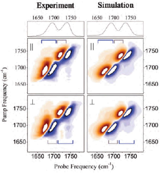
Left column: experimental pump probe spectra of the carbonyls in phospholipid membrane fragments. From top: absorption, and pump probe spectra recorded under parallel and perpendicular polarization conditions of the pump and probe pulses. Right Column: The corresponding simulated spectra. Blue and magenta brackets show the inter- and the intra-band cross-peak regions, respectively [107].
The SOS method described in Sec.III requires the diagonalization of the two-exciton block of the Hamiltonian matrix. The ∼N4 scaling of time and memory computational cost makes it prohibitively expensive for large N. An alternative, quasiparticle scattering, approach greatly reduces the computational cost. This method assumes a molecular Hamiltonian that conserves the number of excitations, and a dipole moment that can only create or annihilate one excitation. The optical transitions are viewed as quasi particles (“excitons”), and the nonlinearity now originates from their collisions.
The amide I Hamiltonian (Eq. (3)) can be approximately recast in terms of Bosonic creation and annihilation operators:
| (30) |
here B †(B) are creation (annihilation) Boson operators, satisfying . The first two terms describe the free excitons where ωm is the local amide I frequency and the Jmn represents the inter-site coupling which induce exciton hopping. Δm and Kmn represent the intra- and inter-site anharmonicity, respectively.
The quasiparticle expressions appear naturally by solving equations of motion, the nonlinear exciton equations (NEE) [62, 64]. A key ingredient is the Green's function, G, which describes the time evolution of two excitons and satisfies the Bethe-Salpeter equation,
| (31) |
G(0) represents the dynamics of two noninteracting excitons. The two-exciton scattering matrix Γ allows to develop powerful approximations and truncation schemes. Its matrix element Γ̄e4e3,e2e1 (Ω) [61] represents the process where two incoming excitons e1 and e2 are scattered to produce e3 and e4.
Formally the computational effort of both the quasiparticle expression and the SOS scale as ∼ N4 with system size. However, a much more favorable scaling is obtained in practice thanks to the localized nature of excitons and their interactions (anharmonicities).[55] To see how this works, we consider the overlap factor of two excitons:
| (32) |
This parameter characterizes the two-exciton configuration in real space: for e = e′ we have η(1)ee′ ≡ 1. For uncoupled vibrations Jmn = 0 and η(1)ee′ = δee′ indicating that the excitons do not interact. Since exciton interactions are short-range (the anharmonicity is local) we can estimate the probability of the scattering event by assuming that exciton pairs (e1e2) can only scatter when their overlap is larger than a certain cutoff ηc : η(1)e1e2 > ηc. The same criterion may also be used for the pairs of outgoing states(e4e3). By applying this cut-off which restricts the distance between two initial and between two final excitons in the scattering matrix the number of relevant scattering matrix, elements should scale as N2N2c rather than N4, where Nc is a finite correlation length; the scattering matrix is sparse.
A second helpful constraint is provided by the exciton-exciton scattering radius which determines how far two-excitons can move during their interaction, and sets bounds on the distance between the initial and final pairs of excitons. We introduce this cutoff by defining a second overlap parameter
| (33) |
η(2) is the amplitude of a path going from e to e′ through all possible intermediate states e1. A cutoff of η(2)
Using both cutoff parameters η(1)C and η(2)C, we can retain only those scattering matrix elements which satisfy η(1)e2e1 >, η(1)C,η(1)e4e3 >, η(1)C,η(1)e4e3 >, η(1)C, η(2)C,η(1)e4e2 >, η(2)C and η(1)e4e1 >, η(2)C. The scaling of the NEE effort with system size thus reduces to ∼N. The efficiency of this truncation stems from two factors: i) The relevant exciton states may be identified before calculating the scattering matrix. Their number is typically much smaller than N4. The scattering matrix should be calculated only for the selected set of scattering configurations. ii) The required numerical effort for computing the signal using multiple summations is reduced considerably by the sparse nature the scattering matrix. The numerical merits of the quasiparticle method become more pronounced as the system size is increased.
Fig. 22 compares the experimental and simulated pump probe spectra for parallel and perpendicular polarization configuration of the pump and the probe pulses, as indicated. The local amide I frequencies are 1708cm−1 (labeled) 1755cm−1 (unlabeled) corrected by a Stark effect frequency shift: Δω = kEproj, where Eproj is the projection of the electric field along the C=O bond. Off-diagonal elements were obtained by using the transition dipole coupling model [149]. The experiment uses a spectrally narrow (16 cm−1) pump and a short (0.1 ps) impulsive probe. The signal field is spectrally dispersed. The experimental bandwidths resulting from the fluctuating electrostatic environment as well as their (diagonally-elongated) shape characteristic to inhomogeneous broadening are reproduced by the simulations. The two strong diagonal resonances correspond to absorption by the two carbonyls.
The cross peak regions in the 2D signal are weak. In order to have a quantitative comparison, the two horizontal sections of the calculated and experimental signals are compared in Fig. 23. The intensities and line shapes of both intra- and inter-band cross-peaks are fairly well reproduced. Each resonance has a negative (blue) contribution due to GSB and ESE, and a positive (red) ESA contribution (Fig. 10. The red shift of the ESA band reflects the anharmonicity of the carbonyl stretching mode. The cross-peaks are more pronounced when the pump and the probe have perpendicular polarization, as shown in Fig. 22. Fig. 23 B depicts horizontal sections of Fig. 22 ║ and ⊥ at the pump frequencies at 1675 and 1752 cm−1 (marked by arrows). The cross-peaks provide a direct measure of vibrational coupling between carbonyl moieties. Structural information such as the distribution of angles between intramolecular carbonyl pairing may be obtained from quantitatively comparing the simulated and experimental result. The pairing geometry is expressed in terms of the angle between the transition dipole moments and of their distance. The vibrational frequencies of the two coupled carbonyls ωn and ωm are obtained by diagonalizing the exciton Hamiltonian
Fig. 23.

A) experimental absorption (thick line) and calculated linear optical absorption (thin line) of DMPC in water. (B) Experimental (open circle lines) and calculated (solid lines) hole-burning spectra under pump excitation at 1675 and 1752 cm−1 (see arrows). Black (parallel) and red (perpendicular) colors indicate the polarization conditions. The perpendicular spectra is magnified by a factor three. Blue and magenta brackets mark the inter- and intra-band cross-peak regions, respectively (see also Figure 22).
| (34) |
These depend on the coupling parameter Jmn and on the difference of the diagonal frequencies, ω0n−ω0m. We further define the pair coupling parameters β′mn
| (35) |
and the weighted radial angular pair distribution function
| (36) |
where the m and n sums run over the 12CO and 13CO carbonyls, respectively.
Fig.24 shows h(R,θ) calculated by considering all 12CO:C13CO pairs(A), only the intermolecular pairs (B), and only the intramolecular pairs (C). Panel A shows that h(R,θ) vanishes for distances of > 6:5 Å implying that the cross peaks are dominated by neighboring carbonyls. The distribution function h(R,θ) (Fig. 24A), consists of several structural families whose intermolecular or intramolecular origin can be easily traced by comparison with Fig.24B and C. The intermolecular h(R,θ) does not show random orientations even when it is broader than its intramolecular counterpart. The sharp peak at θ ≈ 40° and R = 5 Å in Panel C is in agreement with the angle between the transition dipole moments obtained from the experimental anisotropy, suggesting that it is mainly due to intramolecular pairs. We note that for this angle, intermolecular carbonyl pairs also contribute significantly (up to 26 ± 5% to the total h(R,θ) function (see Fig.24).
Fig. 24.

β′ -weighted radial-angular distribution functions (Eq.36) of the simulated DMPC bilayer, calculated considering all 12CO-13CO pairs (A), 12CO-13CO intermolecular pairs (B), and 12CO-13CO intramolecular pairs (C). The red dotted lines indicate the angular values obtained from experimental spectral anisotropy. The chromatic bar shows the range of the statistical distribution according to Eq-36.
These simulations of absorption and pump-probe IR response of carbonyl moieties in a phospholipid bilayer reveal the importance of electrostatic interactions at the polar interface. Both the transition dipole moment coupling and the electric-field fluctuations affect the absorption lineshape. The two contributions, which are convoluted and indistinguishable by the linear response, can be clearly separated in the diagonal and in the off-diagonal parts of the 2D correlation plots. The cross-peak intensity provides a direct measure of the contribution of coupling to the overall line shape. The diagonal elongation results from both the frequency dispersion of the excitonic states and the local electric field fluctuations. The 2D line shapes provide a unique window into the vibrational excitations. The increased degree of localization of the excitonic states in the absorption tails reflects local structural properties of the nearest chromophores.
The quasiparticle-approach adequately describes the 2DIR signatures of structural variations in the phospholipid membranes. This is a promising structural tool for composite phospholipid bilayers, host-guest lipid-protein complexes, lipid systems of reduced dimensionality, and polymers.
VIII. Double-Quantum-Coherence Spectroscopy; The kIII ≡ k1 + k2 - k3 Technique Applied to The TB6 Protein Domain
Elaborate pulse sequences are routinely designed in NMR to exact desired information. Similarly interferences between quantum pathways underlying multi-dimensional signals may be manipulated to design new 2DIR techniques. Here we demonstrate a signal designed to vanish for noninteracting excitons so that it provides an excellent indication for such interactions.
The applications presented so far focused on the kI = !k1+k2+k3 and kII = k1!k2+k3 signals. The kIII = k1+k2!k3 signal carries diRerent types of information. For the exciton model it is given by the two quantum pathways ESA1 and ESA2 shown in Fig. 25. This is analogous to the double quantum coherence technique in NMR [269]. In both diagrams the system is in a coherent superposition between the doubly excited state f and the ground state g during t2. This time-interval thus provides a clean view of two-exciton states. Both (Ω2, Ω3) and (Ω1, Ω2) 2D signals are of interest. Starting with the ground-state (g), each interaction with a laser field can create only one excitation. The first interaction generates a manifold (e) of single-exciton states. The second interaction can either bring the system back to the ground state or can bring the system to the doubly-excited manifold.
Fig. 25.

Double-sided Feynman diagrams representing the Liouville space pathways contributing to the signal in the rotating wave approximation. The first excited state absorption (ESA1) diagram corresponds to R7 and the second excited state absorption (ESA2) diagram to R′4.
As Ω2 is scanned, the signal shows resonances corresponding to the different doubly-excited states f However, the projection along the other axis (Ω3) is different in the two diagrams. In ESA2 the system is in a coherence between e′ and g during t3. As Ω3 is scanned, it reveals single exciton resonances when Ω3 = ωe′g. For ESA1 the system is in a coherence between f and e′ during t3. This gives rise to many new resonances at Ω3 = ωfe corresponding to all possible transitions between doubly and singly excited states. The remarkable point is that for noninteracting excitons the state f is simply given by a direct product of the single pair states e and e′, and the double-excitation energy is the sum of the single-excitation energies and the two diagrams exactly cancel; The resonance pattern of these 2D correlation plots provides a characteristic fingerprint for the correlated nature of two excitons.
The enhanced resolution offered by kIII stems from the absence of diagonal peaks which dominate the kI signal and cover the off diagonal (cross) peaks, and from the doubled frequency-bandwidth of two quantum coherences.
We demonstrate that (Ω2, Ω3) correlation plots of kIII for the the 74-residue TB6 protein domain, [270] TB6, are more sensitive to the couplings, compared with (Ω2, Ω3) correlations in kI . Sensitivity-analysis may be used to assign various regions in congested spectra of globular proteins to specific secondary structures, and separate overlapping regions revealing structural details about protein conformation. We add a small shift ην to the energies ενm of all modes belonging to the ν′th motif (ηνshould be much smaller than all Jmn). The difference of the perturbed and the unperturbed spectrum reflects its sensitivity to this perturbation, and its spectral region can then be assigned to the structure of type ν. gives the simulated kI (SkI)and kIII (SkIII) signal and dissected signal related to helix and hairpin segments and their couplings.
The kIII technique spreads the peaks over a broader range, thus a higher sensitivity to inter-secondary structure couplings and a better resolution.
IX. Putting Chirality into Action; Enhancing The Resolution
Pulse polarizations provide a whole host of convenient control-parameters that may be easily varied in order to manipulate the 2DIR signals. We shall label a coherent heterodyne third order signal, where the 3 incoming pulses are polarized along the v1,v2, v3 directions and the signal is polarized along v4, as vs v3 v2 v1, (Figure 27).
Fig. 27.

Pulse configuration for femtosecond coherent infrared correlation spectroscopy. Three laser pulses (light blue) interact with the sample. The fourth pulse (red) is used to detect its nonlinear response. The control parameters are the time intervals between pulses t1,t2,t3. All pulses propagate along z direction (collinear). The nonchiral signal xxxx is generated when all pulses are polarized along x (blue and red). The CI xxxy signal is obtained by switching the first pulse polarization direction to y (green).
Molecules are typically smaller than the optical wavelength and their response may be adequately described by assuming that the field is uniform across the molecule; this is known as the dipole (or long wavelength) approximation. Our analysis so far was restricted to this limit. We further assumed that all pulses are polarized in parallel and did not specify the pulse polarizations. The nonlinear response then depends on the orientationally-averaged product of four dipoles (μνsm μν3n μν2kμν11). There are only three independent tensor components. These correspond to the polarization configurations: xxyy,xyxy and xyyx. All other configurations can be expressed by their linear combinations.
The variation of the phase of the optical field at different points within the molecule may result in new contributions to the signal. These are caused by interferences among signals generated at different parts of the molecules and are typically 1000 times weaker than the leading (dipole) contributions (this is the ratio of chromophore size to the optical wavelength). However, by choosing certain polarization configurations for which the dipole term vanishes (e.g. xxxy), the non-dipole signals are background-free and may be readily detected. These signals change their signs upon mirror reflection; hence they are finite only for chiral systems and vanish in racemates and in nonchiral molecules.
Circular Dichroism (CD), the difference in the absorption of left and right-handed circularly polarized light [271-273], is the simplest chiral signal. This linear 1D technique is routinely applied for probing the folding states of proteins and their conformational stability. The contributions of different chromophores to CD spectra interfere (the absorption spectrum in contrast is additive and contains no interference). This is the reason for the extra sensitivity to structure, allowing the technique to distinguish between various secondary structures of proteins. Similarly the structural sensitivity of 2D techniques can be greatly enhanced by a judicious choice of chiral polarization configurations. Chirality-induced (CI) 2D techniques extend CD to nonlinear spectroscopy [274, 275]. Chilarity can also be measured by the Raman optical activity technique (ROA) [276], in which a small difference in the Raman intensities induced by right and left circularly polarized incident light is measured. Vibrational CD (VCD) band shapes are characteristic to secondary structures of polypeptides. Protonated α -helical structure give bisignate amide I and A bands [277, 278], and a monosignate amide II band [279]. The amide I has three peaks for right handed helices upon deuteration [279]. α – helix and antiparallel β – sheet are distinguishable by the amide I frequency shift and the band shape change from the tightly overlapped bisignate to two separated negative peaks [280]. Random-coil amide I band shape is also bisignate, but its sign is inverted from α –helix [280, 281]. 310 helix has the higher frequency amide II VCD band and the lower frequency amide II infrared band compared to α – helix, which can be due to the difference in hydrogen bond patterns (4 → 1 vs 5 →1) [282].
The response function for the chirality-induced kI technique depends on the average product [64]:
| (37) |
where jνe(k) is exciton transition dipole in k space:
| (38) |
Molecular chirality originates from the three-dimensional distribution of local transitions in real space. For simplicity, we neglect the local chirality of each peptide unit (due to its magnetic dipole and electronic quadrupole) and only include the global (structural) chirality. Signals sensitive to chirality depend explicitly on the real space coordinates of the various local transitions. We define the transition dipole vector for the zero-momentum exciton state
| (39) |
and the tensor to finite order in k
| (40) |
where rm is the coordinate for the m′th transition, 1m is the transition dipole and Ae;m is the eigenvector. Eq. (38) is independent on rm and insensitive to chirality. Eq. 40 goes beyond the dipole approximation. For components such as xxxx with even number of repeating indices, the first term is finite and will dominate the signal, making it insensitive to chirality. For components with odd number of repeating indices such as xxxy, the first term vanished and the signal is dominated by the other chiral-sensitive terms. The signals depend on products of the form < rν5mnμν4mμν3nμν2kμν1l >. Non-chiral techniques depend on the structure only implicitly through its effect on the frequencies and transition dipoles which affect peak-positions and intensities. The explicit coordinate dependence of the chiral response amplifies the cross-peaks and is the reason why these techniques are more sensitive to fine details of the structure.
There are 3 independent chirality-induced polarization configurations for collinear pulses and 6 additional non collinear terms. [61] The signals further depend on the magnitudes and directions of pulse wavevectors.
Figure 28 shows the simulated infrared chiral response of the amide I vibrations with all beams propagating collinearly along z. The electronic CD spectra given for comparison were simulated using Woody's standard model which includes the electric and magnetic moments of the chromophores [271]. It thus depends on both local and global chirality. The following simulations show how the CI techniques provide complementary information to Circular Dichroism and NMR for a 15 residue hairpin Trpzip4 (Fig 28A) [283], one of the “Tryptophin Zipper” hairpins. Its robust known structure makes it an excellent model for the characterization of the vibrational states of peptides in aqueous solution, for the investigation of the relations of the vibrational spectra with peptide conformations, and for the evaluation of the distributions of structures [283]. The amide I absorption band (Fig 28B) consists of three poorly resolved features; the 1635cm−1 peak and the 1675cm−1 shoulder are related to the b structure [283], while the 1655cm−1 shoulder is related to the turn and coil structures at the two ends. The diagonal peaks of 2D xxxx signals (Fig 28C) resemble the absorption. NMR spectra are routinely used to impose constraints on peptide structure; a distance geometry optimization is then applied to obtain an ensemble of possible conformers consistent with the NMR data [8]. We focus on the first two conformers out of the reported 20 NMR-determined Trpzip4 structures, which have the lowest energy and are thus the best guess of the structure. The RMSD between these two structures is 1.517 A. The calculated electronic (Fig 28D and 28G) and vibrational (Figure 28E and 28H) CD spectra of these conformers are similar. However, the 2D chirality-induced spectra (Figure 28F and 28I) are very different. Conformer I has a strong (1635cm-1,1655cm-1) cross peak while II has a cross peaks at (1655cm-1,1675cm-1).
Fig. 28.
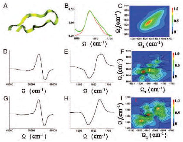
Using chirality-induced 2D correlation spectroscopy to discriminate between the hairpin structures indistinguishable by NMR. (A) Fifteen-residue hairpin peptide Trpzip4. (B) Simulated (red) and experimental (17) (green) absorption of amide I vibrational band. (C) Simulated xxxx 2D signals for the aide I band. (Middle and Bottom) Comparison of the simulated spectra for two configurations drawn from the NMR-determined hairpin structure ensembles. Electronic CD (D and G) of the amide band, vibrational CD (E and H) of the amide I band, and xxxy CI 2D signals (F and I) for the amide I band. The CD signals are similar for the two configurations are shown. Major differences of the2D signals in the cross-peak region indicate specific couplings among vibrational modes.
These examples demonstrate how chirality-induced 2D signals can help determine correlations between different parts of a protein by enhancing crosspeak contributions and help in assigning them to structural features. The crosspeaks are very sensitive to secondary structure variations, and the chiral configuration of different chromophores can be determined from the signs of the corresponding crosspeaks (positive vs. negative crosspeaks between two transitions correspond to different sense of screw configuration of the corresponding transition dipoles). Coherent 2D techniques enhanced by the spatial sensitivity of CI polarization configurations offer a new tool for tracking early protein folding events and pinpointing the average structure and its fluctuations along the folding pathways with femtosecond resolution.
Chirality-induced 2D signals are weaker than their nonchiral counterparts, and have not been observed experimentally so far. Nevertheless being background-free they may be readily detected using state-of-the-art infrared technology. The collinear configuration presented here is the simplest, and can be realized using phase cycling techniques as done in NMR [23-25, 48-55, 63, 269, 284]. Non collinear configurations offer additional possibilities. Combinations of several carefully arranged non collinear experiments may lead to the cancellation of nonchiral terms, so that only the CI terms survive. The pulse configuration may be tailored for probing specific tensor components. For instance, the collinear xxxy signal can be measured in noncollinear geometry whereby all laser beams are arranged in one (yz) plane, the first y-polarized beam propagate along z and the other x-polarized beams can have wavevector component along y. All non-chiral contributions vanish for this configuration and only xxxy survives.
X. The Structure of Amyloid Fibrils; Manipulating 2D Signals by Coherent-Control Techniques
The accumulation of amyloid deposits, [285] whose dominant component is a 39-43 residue A β peptide, [286] has been identified as a major feature of the pathogenesis of Alzheimer's disease (AD). [287] Despite their identical 1-39 sequence, the various Aβ peptides have significantly different biochemical properties: The 42-residue derivative Aβ 42 deposits much faster than others and the fibrils formed are more stable. [288] Aβ 42 is also slightly more hydrophobic, compared with shorter analogs such as Aβ 40, because of the two additional more-hydrophobic residues at the end of the peptide strand. [289] More importantly, the protease resistance of Aβ 42 is drastically different from its analogs. [289].
The structural basis of these property differences is still unknown. Because of the fibrils noncrystalline, insoluble, and mesoscopically heterogeneous nature, NMR rather than x-ray is the primary tool for fibril structure determination [285, 290]. NMR provides various structural constraints that, when combined with computational tools, such as geometry optimization and MD simulations, yield the plausible structural models. The most recent model of Aβ 42 structure was proposed by Riek [290] (denoted M42). M42 can be dissected into 3 motifs; residues 1-16 are randomly coiled, residues 26-31 are the turn and the rest form two β strands. NMR structural information (7, 10) is primarily related to the β -strand. For the lack of structural constraints, the turn structure in this model is obtained by geometry optimization and depends heavily on the computational protocol and the empirical force field. 2D IR were reported recently [109, 110].
The simulated absorption of M42 (Fig-29 Left, Abs) shows an intense ∼1, 635cm−1 peak (peak a), an ∼1; 655cm−1 shoulder (peak b), an ∼1, 675cm−1 peak, two additional peaks at ∼1; 695cm−1 (peak d) and ∼ 1; 715cm−1 (peak i). Fig-29 Left (NMD) shows the decomposition of the various normal modes into the three structural motifs (β -sheet, turn, and coil). Peaks a, b, and c have strong contributions from both β -strand and coil. d has a contribution from turn plus coil, and i is purely turn. Fig-29 Left (2D), displays simulated xxyy 2DCS signals. The signal is dominated by strong and broad diagonal peaks that resemble the absorption no cross-peaks are observed. The contributions of all three structural motifs overlap. The lower resolution and normal mode delocalization complicate the interpretation of the cross peak compared with NMR. However, isotope-labeling combined with a judicious design of polarization configurations can be used to manipulate the 2DCS signals by enhancing desired spectral features. 13C18O isotope labeling of a given peptide residue can induce a 65 cm−1 red shift of the amide-I vibrational frequency, creating peaks well separated from the unlabeled band and providing structural information on desired segments. Two-dimensional signals depend on interferences among many contributions (Liouville space pathways).
Fig. 29.

Left: From top to bottom: the NMD diagram, the absorption signal (Abs), the xxyy polarization 2DCS (2D), and the coherent-controloptimized- polarization [2D(CP) ] 2DCS of unlabeled M42 amyloid. In NMD, the β -strand, coil, and turn content are shown in red, green, and blue, respectively. Right: same quantities for coil-labeled fibril.
This interference may be controlled by varying the relative polarizations of the various beams, thereby eliminating diagonal peaks and amplifying the cross-peaks. Below we demonstrate how a coherent control algorithm may be used to manipulate the 2DIR feature of Aβ 42, creating well-resolved cross peaks which is directly related to interactions within turn segments and between turn and β -sheet, thus make it possible to propose additional constraints for the turn structure.
To suppress the diagonal 1655 cm-1 peak, we have constructed the following superposition of the three linearly independent tensor components Tj = xxyy; xyxy; xyyx:
| (41) |
The complex coefficients cj were optimized using a genetic algorithm [291] aimed at minimizing the control target: the ratio of the integrated diagonal line in the absolute magnitude of the 2D spectrum to the integrated diagonal peak at 1655 cm-1 with δ = 10cm−1. Fast exponential convergence was achieved using 10 members in a population within 100-200 generations. The noise reduction parameter [291] was ε = 0.6 – 0.7, and the parameters of the selection: Li = 5, Lf = 6. The optimized coefficients for M40 in figure 1 are: c1 =0.14-i*0.35, c2=0.16-i*0.79, c3= -0.27-i*0.36. For M42 in figure 1 are: c1= -0.34-i*0.56, c2=-0.044-i*0.54, c3=0.34-i*0.40. For M42 in figure 3 are: c1= 0.57+i*0.28, c2= 0.04+i*0.22,c3= -0.59-i*0.44. A much richer cross-peak pattern is seen in the signal [Fig-29 Left, 2D(CP)] compared with the noncontrolled xxxx signal (Fig-29 Left, 2D).
The (CP) signal of M42 shows two strong cross peaks related to the correlation between the d and i absorption features. These are displayed in Fig-30 on an expanded scale and marked AB-1 (1695,1715) and AB-2 (1715,1695). The normal modes contributing to the diagonal peaks were projected onto the local amide modes along the backbone in order to assign the cross peaks to positions along the structure. The i modes (Fig 30 A:1715) are dominantly localized within the turn segment and residue 28 has the largest weight, while the d modes (Fig 30 B:1695) are almost evenly distributed among the coil and the 28-30 residues of the turn. Given the large distance between the coil and the turn, (see Fig 30) we expect their interaction to be negligible. We thus conclude that these two cross peaks reflect turn-turn interactions, especially within the 28-30 residue.
Fig. 30.

Above the dash line: The 2DCS signal of M42 with Coherent-control-optimized polarization configuration (Fig 29 middle left panel) on an expanded scale (1630-1730) and the projection of the normal modes contributing to the specified cross peaks onto the local amide modes along the backbone. The population is an average over a given residues on each layer [Sentence not clear]. Below the dash line: Same for coil labeled M42. in the 2DCS plot, the cross peaks (blue arrows) are attributed to the turn-turn interaction, red turn-sheet and black sheet-sheet. In the normal mode projection plots, the turn contribution is shown in blue, sheet (red) and coil (green). Green arrows above the 2DCS denote absorption peak positions.
Most peaks in the M42 spectra contain significant contributions from more than one structural motif and may not be assigned unambiguously Upon isotope-labeling of the coil segment (residue 1-16), the peaks will be dominated by one structural motif composition
(Fig 29 NMD). The newly-appeared shoulder e in the linear absorption (Fig 29 Abs) is 67 dominated by the coil segment. a,b and c are all dominated by the sheet and d,i belong to the turn, as can be seen in the top panel. The 2DCS (Fig 29 2D) has a better cross peak resolution than in the unlabeled sample, but the main cross peak pattern is still unresolved. The same coherent-control protocol may be employed to eliminate the diagonal peak of the isotopically labeled peptide at 1655 cm-1 (Fig29 2D(CP)). Most cross peaks may now be clearly assigned.
Fig 30 C:1715 and D:1695 demonstrate that for the coil-labeled sample, peak d and I are both dominated by the turn, the cross peaks CD1 (1695,1715) and CD2 (1715,1695) are thus related to turn-turn interactions. Fig 30 H:1615 and G:1635 shows that the 1615 cm-1 and 1635 cm-1 frequency windows are dominated by the strand motif. The CH, DH and CG cross peaks thus originate from interactions between the turn and the sheet motifs close to the turn segment (mainly residue 24-25 and residue 32-33). The normal modes in the 1675 cm-1 window (Fig30 E:1675) are also dominated by the sheet motif, the local mode population is rather non-uniformly distributed and there is no contribution from mode 25. CE thus primarily originates from the interaction between the turn and residue 32. The normal modes 1655 cm-1 (Fig30 F:1655), however, have a significant contribution from both the sheet and the turn, thus the CF,DF1,DF2 peaks should contain mixed information about turn-turn and turn-sheet interaction. The additional cross peaks FF and FH, marked by black arrows are related to sheet-sheet interactions.
XI. Summary and Future Outlook
Most 2DIR experiments performed so far focused on a few nonequilibrium studied were described in the introduction. The computational arsenal presented here may be readily applied to describe nonequilibrium processes initiated by fast triggering, provided they are slower than a typical 2D measurement timescale (∼200 fs). We can then assume that the system is stationary during the measurement but characterized by time-dependent parameters related to the process under study (e.g. protein folding, photochemically triggered conformational change, and hydrogen-bond breaking). 2D spectra could then provide stroboscopic snapshots of these processes. The numerical propagation (Fig. 20) and the SLE techniques are not restricted to this limit and may be used to describe an arbitrary nonstationary initial state, irrespective of the timescale (fast or slow dynamics compared to the measurement).
It will be instructive to point out some analogies between 2D and single-molecule spectroscopies [292]. In the course of time, each molecule in an ensemble undergoes a stochastic evolution and its properties e.g. frequencies, orientations, dipole moments fluctuate due to couplings with uncontrollable external “bath” degrees of freedom. Bulk measurements probe the ensemble average of these stochastic trajectories. Single molecule spectroscopy dissects the ensemble by brute force: observing individual trajectories one molecule at a time. It thus provides considerably more detailed information than bulk measurements. Nonlinear spectroscopy accomplishes a similar goal by observing the entire ensemble but at multiple time points. There are many possible microscopic models with very different types of trajectories that could yield the same ensemble-average at a given time. The multipoint correlation functions obtained by nonlinear spectroscopy have the capacity to distinguish between such models. Even though individual trajectories are not observed. Consider for example a chemically reactive system at equilibrium A-B. If the reaction rates are slow on the spectroscopic time scale, the absorption spectrum will be simply given by the weighted average of species A and B; No information about the kinetics is available from 1D spectroscopy. In a 2D measurement one can vary the time delay t2 on the kinetic timescale and extract the kinetics from the time evolution of the cross peaks. The cross peaks give the conditional probability of the system to be in A during t1 and B during t3. Typically t1 and t3 are much shorter than t2. This is therefore a measurement at two-points separated by t2. This is complementary to triggered experiments where we perturb the system out of equilibrium and watch the subsequent relaxation. [92, 293] SMS is a long (msec and longer) time-measurement. 2DIR can provide trajectory information on the fsec timescale. A common thread to both techniques is the analysis in terms of ensembles of trajectories rather than of configurations[294].
Over the past decade, 2DIR has established itself as a useful spectroscopic tool for the investigation of molecular structures and ultrafast molecular events. The technique has a lower structural resolution than NMR, but its unique high temporal resolution and different observation window make it an invaluable complementary tool to NMR.
Early efforts were at the proof of concept stage and focused on demonstrating the various capabilities and potentials of this technique current activity in the field focuses on identifying specific systems where 2DIR can be particularly helpful, and developing the necessary protocols for quantitatively analyzing the 2DIR signals are thus major challenges in the field. A concerted experimental and the theoretical effort, will be required on benchmark systems to improve the current protocols. We expect it to go through a similar deavelopment trajectory to the history of classical force field for Molecular Mechanic simulations.
As a step in this direction, our group is developing a computational package \SPECTRON″, which is a C/C++ software designed to give a unified platform for optical spectroscopy calculations. It is available to the research community. We aim at calculating a broad range of linear and nonlinear optical signals of complex biomolecules. SPECTRON currently includes the modules for constructing Hamiltonians for (i) the amide I,II,III,A vibrational bands and n-.., .-.. electronic bands for peptides based on MD simulation trajectory (ii) the C=O stretch in guanine, the in-plane or out-of-plane, symmetric or asymmetric NH or NH2 bend in adenine, the ring C=N stretch in cytosine for RNAs based on MD simulation trajectories. (iii) the O-H stretching band of water based on MD simulation trajectory. (iv) C-O stretching band of membrane lipids based on MD simulation trajectory. An interface between SPECTRON and standard MD simulation packages such as CHARMM [58], NAMD [295] and GROMOS [59] is constructed so that the MD simulation trajectories in ASCII or binary formats can be directly read. This will make it accessible to both the MD simulation community and ultrafast spectroscopists. With the Hamiltonian constructed, SPECTRON can be used to calculate various signals including absorption, photon echo (kI), pump probe, double quantum signal (kIII) and second order signals using SOS and the quasiparticle approaches. Separate codes for calculating these signals using Numerical Propagation (NP) and Stochastic Liouville Equations (SLE) will be merged into the package.
Fig. 26.
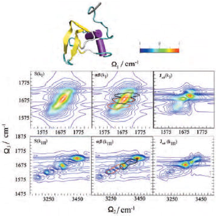
Top row: Simulated signal and sensitivity analysis for the kI signal of TB6 protein domain. SkI is the signal. αβ (kI) gives the regions related to α helix (red contour) and β sheet (black contour). J αβ (kI) gives the region related to the coupling between α helix (red contour) and β sheet. Bottom row: same quantities for the KIII signal.
Acknowledgments
This work was supported by the National Institutes of Health Grant GM59230 and the National Science Foundation Grant CHE-0745891. W.Z thanks UCI Dissertation Fellowship for financial support. Many helpful discussions with Drs. Darius Abramavicius, Cyril Falvo and Lijun Yang are gratefully acknowledged.
References
- 1.Stryer L. Biochemistry. 2nd W.H.Freeman Company; New York: 1995. [Google Scholar]
- 2.Rhodes Gale. A Guide for Users of Macromolecular Models. Third. Academic Press; Burlington: 2006. Crystallography Made Crystal Clear. [Google Scholar]
- 3.Segel DJ, Bachmann A, Hofrichter J, Hodgson KO, Doniach S, Kiefhaber T. J Mol Bio. 1999;288:489. doi: 10.1006/jmbi.1999.2703. [DOI] [PubMed] [Google Scholar]
- 4.Arai S, Hirai M. Biophysical J. 1999;76(4):2192–2197. doi: 10.1016/S0006-3495(99)77374-1. [DOI] [PMC free article] [PubMed] [Google Scholar]
- 5.Pollack L, Tate MW, Darnton NC, Knight JB, Gruner SM, Eaton WA, Austin RH. Proc Natl Acad Sci USA. 1999;96:10115–10117. doi: 10.1073/pnas.96.18.10115. [DOI] [PMC free article] [PubMed] [Google Scholar]
- 6.Uzawa T, Kimura T, Ishimori K, Morishima I, Matsui T, Ikeda-Saito M, Takahashi S, Akiyama S, Fujisawa T. J Mol Biol. 2006;357:997–1008. doi: 10.1016/j.jmb.2005.12.089. [DOI] [PubMed] [Google Scholar]
- 7.Pfuhl M, Driscoll PC. Philosophical Transactions of the Royal Society of London Series a-Mathematical Physical and Engineering Sciences. 2000;358(1766):513–545. doi: 10.1098/rsta.2000.0536. [DOI] [PMC free article] [PubMed] [Google Scholar]
- 8.Wutrich K. NMR of proteins and Nucleic Acids. Wiley; New York: 1995. [Google Scholar]
- 9.Gruenewald B, Nicola CU, Lustig A, Schwarz G, Klump H. Biophysical Chemistry. 1979;9(2):137–147. doi: 10.1016/0301-4622(79)87008-8. [DOI] [PubMed] [Google Scholar]
- 10.Ernst Richard R, Bodenhausen GeoRrey, Wokaun Alexander. Principles of Nuclear Magnetic Resonance in One and Two Dimensions. Vol. 14. Clarendon; Oxford: 1987. (The International Series of Monographs on Chemistry). [Google Scholar]
- 11.Rose-Petruck C, Jimenez R, Guo T, Cavalleri A, Siders CW, Raksi F, Squier JA, Walker BC, Wilson KR, Barty CPJ. Nature. 1999;398:310–312. [Google Scholar]
- 12.Zewail AH, Chergui M. Angew Chem. 2008 submitted. [Google Scholar]
- 13.Zewail Ahmed H. Physical Biology, From Atoms to Medicine. Imperial College Press; London: 2008. [Google Scholar]
- 14.Eaton WA, Munoz V, Hagen SJ, Jas GS, Lapidus LJ, Henry ER, Hofrichter J. Annual Review of Biophysics and Biomolecular Structure. 2000;29:327–359. doi: 10.1146/annurev.biophys.29.1.327. [DOI] [PMC free article] [PubMed] [Google Scholar]
- 15.Chalmers JM, Griffiths PR, editors. Handbook of vibrational spectroscopy. John Wiley & Sons Ltd.; New York: 2002. Applications of Vibrational Spectroscopy in Life, Pharmaceutical and Natural Sciences. [Google Scholar]
- 16.Hein M, Wegener AA, Engelhard M, Siebert F. Biophys J. 2003;84:1208–1217. doi: 10.1016/S0006-3495(03)74935-2. [DOI] [PMC free article] [PubMed] [Google Scholar]
- 17.Brudler R, Rammelsberg R, Woo TT, GetzoR ED, Gerwert K. Nature Structural Biology. 2001;8:265–270. doi: 10.1038/85021. [DOI] [PubMed] [Google Scholar]
- 18.Aki M, Ogura T, Shinzawa-Itoh K, Yoshikawa S, Kitagawa T. J Phys Chem. 2000;104:10765–10774. [Google Scholar]
- 19.Asher SA, Ianoul A, Mix G, Boyden MN, Karnoup A, Diem M, Schweitzer-Stenner R. J Am Chem Soc. 2001;123:11775–11781. doi: 10.1021/ja0039738. [DOI] [PubMed] [Google Scholar]
- 20.Blanch EW, Morozova-Roche LA, Cochran DAE, Doig AJ, Hecht L, Barron L. J Mol Biol. 2000;301:553–563. doi: 10.1006/jmbi.2000.3981. [DOI] [PubMed] [Google Scholar]
- 21.Cho MH. Chem Rev. 2008;108:1331–1418. doi: 10.1021/cr078377b. [DOI] [PubMed] [Google Scholar]
- 22.Bredenbeck J, Helbing J, Kolano C, Hamm P. Chemphyschem. 2007;8:1747–1756. doi: 10.1002/cphc.200700148. [DOI] [PubMed] [Google Scholar]
- 23.Scheurer C, Mukamel S. J Chem Phys. 2001;115:4989. [Google Scholar]
- 24.Scheurer C, Mukamel S. J Chem Phys. 2002;116:6803–6816. [Google Scholar]
- 25.Scheurer C, Mukamel S. Bull Chem Soc Jpn. 2002;75:989–999. [Google Scholar]
- 26.Kwak KW, Park S, Fayer MD. Proc Natl Acad Sci USA. 2007;104:14221–14226. doi: 10.1073/pnas.0701710104. [DOI] [PMC free article] [PubMed] [Google Scholar]
- 27.Venkatramani R, Mukamel S. J Chem Phys. 2002;117:11089. [Google Scholar]
- 28.(2007) Chem. Phys. 341(1-3 (Special Issue. Ultrafast Dynamics of Molecules in the Condensed Phase:Photon Echos and Coupled Excitations: A Tribute to Douwe A. Wiersma)).
- 29.Zhao W, Wright JC. J Am Chem Soc. 1999;121:10994–10998. [Google Scholar]
- 30.Shakhnovich EI. Current Opinion in Structural Biology. 1997;7(1):29–40. doi: 10.1016/s0959-440x(97)80005-x. [DOI] [PubMed] [Google Scholar]
- 31.Karplus M, McCammon JA. Nature Structural Biology. 2002;9(9):646–652. doi: 10.1038/nsb0902-646. [DOI] [PubMed] [Google Scholar]
- 32.McCammon JA, Harvey SC. Dynamics of Proteins and Nucleic Acids. Cambridge University Press; Cambridge: 1987. [Google Scholar]
- 33.Daura X, Gademann K, Schafer H, Jaun B, Seebach D, van Gunsteren WF. J Am Chem Soc. 2001;123:2393–2404. 2404. doi: 10.1021/ja003689g. [DOI] [PubMed] [Google Scholar]
- 34.Onuchic JN, LutheySchulten Z, Wolynes PG. Annu Rev Phys Chem. 1997;48:545–600. doi: 10.1146/annurev.physchem.48.1.545. [DOI] [PubMed] [Google Scholar]
- 35.Bryngelson JD, Onuchic JN, Socci ND, Wolynes PG. Proteins-Structure Function and Genetics. 1995;21(3):167–195. doi: 10.1002/prot.340210302. [DOI] [PubMed] [Google Scholar]
- 36.Wolynes PG, Onuchic JN, Thirumalai D. Science. 1995;267(5204):1619–1620. doi: 10.1126/science.7886447. [DOI] [PubMed] [Google Scholar]
- 37.Gnanakaran S, Nymeyer H, Portman J, Sanbonmatsu KY, Garcia AE. Current Opinion in Structural Biology. 2003;13(2):168–174. doi: 10.1016/s0959-440x(03)00040-x. [DOI] [PubMed] [Google Scholar]
- 38.Duan Y, Kollman P. Science. 1998;282:740. doi: 10.1126/science.282.5389.740. [DOI] [PubMed] [Google Scholar]
- 39.Wang J, Onuchic J, Wolynes P. Phys Rev Lett. 1996;76:4861–4864. doi: 10.1103/PhysRevLett.76.4861. [DOI] [PubMed] [Google Scholar]
- 40.Snow CD, Zagrovic B, Pande VS. J Am Chem Soc. 2002;124(49):14548–14549. doi: 10.1021/ja028604l. [DOI] [PubMed] [Google Scholar]
- 41.Freddolino Peter L, Liu Feng, Gruebele Martin, Schulten Klaus. Biophys J. 2008 doi: 10.1529/biophysj.108.131565. [DOI] [PMC free article] [PubMed] [Google Scholar]
- 42.Zhu Y, Alonso DOV, Maki K, Huang CY, Lahr SJ, Daggett V, Roder H, DeGrado WF, Gai F. Proc Natl Acad Sci USA. 2003;100(26):15486–15491. doi: 10.1073/pnas.2136623100. [DOI] [PMC free article] [PubMed] [Google Scholar]
- 43.Kubelka J, Eaton WA, Hofrichter J. J Mol Biol. 2003;329(4):625–630. doi: 10.1016/s0022-2836(03)00519-9. [DOI] [PubMed] [Google Scholar]
- 44.Snow CD, Nguyen N, Pande VS, Gruebele M. Nature. 2002;420(6911):102–106. doi: 10.1038/nature01160. [DOI] [PubMed] [Google Scholar]
- 45.Frenkel D, Smit B. Understanding molecular simulation:from algorithms to applications 2002 [Google Scholar]
- 46.Mohanty D, Elber R, Thirumalai D, Beglov D, Roux B. J Mol Biol. 1997;272:423–442. doi: 10.1006/jmbi.1997.1246. [DOI] [PubMed] [Google Scholar]
- 47.Dellago C, Bolhuis P, Csajka F, Chandler D. J Chem Phys. 1998;108:1964–1977. [Google Scholar]
- 48.Chernyak V, Zhang WM, Mukamel S. J Chem Phys. 1998;109:9587. [Google Scholar]
- 49.Mukamel S, Piryatinski A, Chernyak V. J Chem Phys. 1999;110:1711. [Google Scholar]
- 50.Piryatinski A, Tretiak S, Chernyak V, Mukamel S. J Raman Spec. 2000;31:125–135. [Google Scholar]
- 51.Piryatinski, Chernyak V, Mukamel S. In: Two-dimensional coherent infrared spectroscopy of vibrational excitons in polypeptides, in Ultrafast Infrared and Raman Spectroscopy. Fayer M, editor. Marcel Dekker Inc.; New York: 2001. pp. 349–382. [Google Scholar]
- 52.Piryatinski A, Chernyak V, Mukamel S. Chem Phys. 2001;266:311. [Google Scholar]
- 53.Scheurer C, Piryatinski A, Mukamel S. J Am Chem Soc. 2001;123:3114. doi: 10.1021/ja003412g. [DOI] [PubMed] [Google Scholar]
- 54.Piryatinski A, Asher SA, Mukamel S. J Phys Chem A. 2002;106:3524–3530. [Google Scholar]
- 55.Zhuang W, Abramavicius D, Hayashi T, Mukamel S. J Phys Chem B. 2006;108(46):18034–18045. doi: 10.1021/jp055813u. [DOI] [PMC free article] [PubMed] [Google Scholar]
- 56.Wang JP, Chen JX, Hochstrasser RM. J Phys Chem B. 2006;110:7545–7555. doi: 10.1021/jp057564f. [DOI] [PMC free article] [PubMed] [Google Scholar]
- 57.Demirdoven N, Cheatum CM, Chung HS, Khalil M, Knoester J, Tokmako R A. J Am Chem Soc. 2004;126(25):7981–7990. doi: 10.1021/ja049811j. [DOI] [PubMed] [Google Scholar]
- 58.Brooks BR, Bruccoleri RE, Olafson BD, States DJ, Swaminathan S, Karplus M. J Comput Chem. 1983;4:187–217. [Google Scholar]
- 59.Scott WRP, Hunenberger PH, Tironi IG, Mark AE, Billeter SR, Fennen J, Torda AE, Huber T, Kruger P, van Gunsteren WF. J Phys Chem A. 1999;103:3596–3607. [Google Scholar]
- 60.Pearlman DA, Case DA, Caldwell JW, Ross WS, Cheatham TE, Debolt S, Ferguson D, Seibel G, Kollman P. Computer Physics Communications. 1995;91:1–41. [Google Scholar]
- 61.Abramavicius D, Mukamel S. J Chem Phys. 2005;122(13):134305. doi: 10.1063/1.1869495. [DOI] [PubMed] [Google Scholar]
- 62.Mukamel S, Abramavicius D. Chem Rev. 2004;104(4):2073–2098. doi: 10.1021/cr020681b. [DOI] [PubMed] [Google Scholar]
- 63.Mukamel S. In: Many-body eRects in nonlinear susceptibilities; beyond the local-field approximation, in Molecular Nonlinear Optics. Zyss J, editor. Academic Press; New York: 1994. pp. 1–46. [Google Scholar]
- 64.Abramavicius D, Palmieri B, Voronine V, ^Sanda F, Mukamel S. Chem Rev (submitted) 2008 doi: 10.1021/cr800268n. [DOI] [PMC free article] [PubMed] [Google Scholar]
- 65.Mukamel S. Annu Rev Phys Chem. 2000;51:691–729. doi: 10.1146/annurev.physchem.51.1.691. [DOI] [PubMed] [Google Scholar]
- 66.Mukamel S. Principles of Nonlinear Optical Spectroscopy. Oxford University Press; New York: 1995. [Google Scholar]
- 67.Laubereau A, Kaiser W. Reviews of Modern Physics. 1978;50:607–665. [Google Scholar]
- 68.George SM, Harris AL, Berg M, Harris CB. J Chem Phys. 1984;80:83–94. [Google Scholar]
- 69.Allen L, Elberly JH. Optical Resonances and Two-Level Atoms. Wiley; New York: 1975. [Google Scholar]
- 70.Loring RF, Mukamel S. J Chem Phys. 1985;83:2116–2128. [Google Scholar]
- 71.Muller LJ, Vandenbout D, Berg M. J Chem Phys. 1993;99:810–819. [Google Scholar]
- 72.Vandenbout D, Muller LJ, Berg M. Phys Rev Lett. 1991;67:3700–3703. doi: 10.1103/PhysRevLett.67.3700. [DOI] [PubMed] [Google Scholar]
- 73.Muller M, Wynne K, Vanvoorst JDW. Chem Phys. 1988;125:225–230. [Google Scholar]
- 74.Mukamel S. Phys Rev A. 1983;28:3480. [Google Scholar]
- 75.Mukamel S, Loring RF. J Opt Soc Am B. 1986;3:595–606. [Google Scholar]
- 76.Fried LE, Mukamel S. Advances in Chem Phys. 1993;84:435. [Google Scholar]
- 77.Tanimura Y, Mukamel S. J Chem Phys. 1993;99:9496. doi: 10.1063/1.2727445. [DOI] [PubMed] [Google Scholar]
- 78.Kaufman LJ, Heo J, Ziegler LD, Fleming GR. Phys Rev Lett. 2002;88:207402. doi: 10.1103/PhysRevLett.88.207402. [DOI] [PubMed] [Google Scholar]
- 79.Kubarych K, Milne CJ, Miller RJD. Chem Phys Lett. 2003;369:635. [Google Scholar]
- 80.Saito S, Ohmine I. J Chem Phys. 1998;108:240. [Google Scholar]
- 81.Ma A, Stratt RM. J Chem Phys. 2002;116:4972. [Google Scholar]
- 82.Okumura K, TokmakoR A, Tanimura Y. J Chem Phys. 1999;111:492. [Google Scholar]
- 83.Mukamel S, Piryatinski A, Chernyak V. Acc Chem Res. 1999;32:145. [Google Scholar]
- 84.Miller RD, Muriname MM, Scherer NF, Weiner AM, editors. Ultrafast Phenomena XIII. Springer; Berlin/Heidelberg: 2002. [Google Scholar]
- 85.Jansen TlC, Duppen K, Snijders JG. Phys Rev B. 2003;67:134206. [Google Scholar]
- 86.Saito S, Ohmine I. J Chem Phys. 2003;119:9073–9087. [Google Scholar]
- 87.Milne CJ, Li Y, Miller RJD. In: Two Dimensional 5th-order Raman Spectroscopy, in Time-Resolved Spectroscopy in Complex Liquids. Torre R, editor. Springer-Verlag; New York: 2007. p. 1. [Google Scholar]
- 88.Palese S, Buontempo JT, Schilling L, Lotshaw WT, Tanimura Y, Mukamel S, Miller RJD. J Phys Chem. 1994;98:12466–12470. [Google Scholar]
- 89.Li YL, Huang L, Miller RJD, Hasegawa T, Tanimura Y. J Chem Phys. 2008 doi: 10.1063/1.2927311. [DOI] [PubMed] [Google Scholar]
- 90.Zhang WM, Chernyak V, Mukamel S. J Chem Phys. 1999;110:5011. [Google Scholar]
- 91.Asplund MC, Zanni MT, Hochstrasser RM. Proc Natl Acad Sci USA. 2000;97(15):8219–8224. doi: 10.1073/pnas.140227997. [DOI] [PMC free article] [PubMed] [Google Scholar]
- 92.Kolano C, Helbing J, Kozinski M, Sander W, Hamm P. Nature. 2006;444(7118):469–472. doi: 10.1038/nature05352. [DOI] [PubMed] [Google Scholar]
- 93.Mukherjee P, Kass I, Arkin I, Zanni MT. Proc Natl Acad Sci USA. 2006;103:3528–3533. doi: 10.1073/pnas.0508833103. [DOI] [PMC free article] [PubMed] [Google Scholar]
- 94.Brixner T, Stenger J, Vaswani HM, Cho M, Blankenship RE, Fleming GR. Nature. 2005;434(7033):625–628. doi: 10.1038/nature03429. [DOI] [PubMed] [Google Scholar]
- 95.Hybl JD, Christophe Y, Jonas DM. Chem Phys. 2001;266:295. [Google Scholar]
- 96.Li XQ, Zhang TH, Borca CN, CundiR ST. Phys Rev Lett. 2006;96:57406. doi: 10.1103/PhysRevLett.96.057406. [DOI] [PubMed] [Google Scholar]
- 97.Zhang TH, Kuznetsova I, Meier T, Li XC, Mirin RP, Thomas P, CundiR ST. Proc Natl Acad Sci USA. 2007;104:14227–14232. doi: 10.1073/pnas.0701273104. [DOI] [PMC free article] [PubMed] [Google Scholar]
- 98.Hamm P, Lim MH, Hochstrasser RM. J Phys Chem B. 1998;102:6123. [Google Scholar]
- 99.Hamm P, Lim M, DeGrado WF, Hochstrasser RM. P Natl Acad Sci. 1999;96:2036–2041. doi: 10.1073/pnas.96.5.2036. [DOI] [PMC free article] [PubMed] [Google Scholar]
- 100.Woutersen S, Hamm P. J Phys Chem B. 2000;104(47):11316–11320. [Google Scholar]
- 101.Zanni MT, Asplund MC, Hochstrasser RM. J Chem Phys. 2001;114(10):4579–4590. [Google Scholar]
- 102.Fang C, Wang J, Kim YS, Charnley AK, Barber-Armstrong W, Smith AB, Decatur SM, Hochstrasser RM. J Phys Chem B. 2004;108:10415–10427. [Google Scholar]
- 103.Maekawa H, Toniolo C, Moretto A, Broxterman QB, Ge NH. J Phys Chem B. 2006;110:5834–5837. doi: 10.1021/jp057472q. [DOI] [PubMed] [Google Scholar]
- 104.Krummel AT, Mukherjee P, Zanni MT. J Phys Chem B. 2003;107:9165–9169. [Google Scholar]
- 105.Larsen OFA, Bodis P, Buma WJ, Hannam JS, Leigh DA, Woutersen S. Proc Natl Acad Sci USA. 2005;102(38):13378–13382. doi: 10.1073/pnas.0505313102. [DOI] [PMC free article] [PubMed] [Google Scholar]
- 106.Ganim Z, Chung HS, Smith AW, DeFlores LP, Jones KC, Tokmakoff A. Acc Chem Res. 2008;41:432–441. doi: 10.1021/ar700188n. [DOI] [PubMed] [Google Scholar]
- 107.Volkov V, Chelli R, Zhuang W, Nuti F, Takaoka Y, Papini AM, Mukamel S, Righini R. P Natl Acad Sci USA. 2007;104:15323–15327. doi: 10.1073/pnas.0706426104. [DOI] [PMC free article] [PubMed] [Google Scholar]
- 108.Bredenbeck J, Ghosh A, Smits M, Bonn M. J Am Chem Soc. 2008;130:2152. doi: 10.1021/ja710099c. [DOI] [PubMed] [Google Scholar]
- 109.Shim SH, Strasfeld DB, Ling YL, Zanni MT. Proc Natl Acad Sci USA. 2007;104(36):14197–14202. doi: 10.1073/pnas.0700804104. [DOI] [PMC free article] [PubMed] [Google Scholar]
- 110.Paul C, Wang JP, Wimley WC, Hochstrasser RM, Axelsen PH. J Am Chem Soc. 2004;126:5843–5850. doi: 10.1021/ja038869f. [DOI] [PMC free article] [PubMed] [Google Scholar]
- 111.Kim YS, Liu L, Axelsen PH, Hochstrasser RM. Proc Natl Acad Sci USA. 2008;105:7720–7725. doi: 10.1073/pnas.0802993105. [DOI] [PMC free article] [PubMed] [Google Scholar]
- 112.Bredenbeck J, Helbing J, Behrendt R, Renner C, Moroder L, Wachtveitl J, Hamm P. J Phys Chem B. 2003;107:8654–8660. [Google Scholar]
- 113.Chung HS, Ganim Z, Jones KC, TokmakoR A. Proc Natl Acad Sci USA. 2007;104:14237–14242. doi: 10.1073/pnas.0700959104. [DOI] [PMC free article] [PubMed] [Google Scholar]
- 114.Bredenbeck J, Helbing J, Kumita JR, Woolley GA, Hamm P. Proc Natl Acad Sci USA. 2005;102:2379–2384. doi: 10.1073/pnas.0406948102. [DOI] [PMC free article] [PubMed] [Google Scholar]
- 115.Broquier M, Crepin C, Dubost H, Galaup JP. Chem Phys. 2007;341:207–217. doi: 10.1021/jp0509921. [DOI] [PubMed] [Google Scholar]
- 116.Bandaria JN, Dutta S, Hill SE, Kohen A, Cheatum CM. J Am Chem Soc. 2008;130:220. doi: 10.1021/ja077599o. [DOI] [PMC free article] [PubMed] [Google Scholar]
- 117.Cahoon JF, Sawyer KR, Schlegel JP, Harris CB. Science. 2008;319:1820–1823. doi: 10.1126/science.1154041. [DOI] [PubMed] [Google Scholar]
- 118.Deak JC, Rhea ST, Iwaki LK, Dlott DD. J Phys Chem A. 2000;104:4866–4875. [Google Scholar]
- 119.Dlott DD. Chem Phys. 2001;266:149–166. [Google Scholar]
- 120.Fecko CJ, Eaves JD, Loparo JJ, TokmakoR A, Geissler PL. Science. 2003;301:1698–1702. doi: 10.1126/science.1087251. [DOI] [PubMed] [Google Scholar]
- 121.Eaves JD, Loparo JJ, Fecko CJ, Roberts ST, TokmakoR A, Geissler PL. Proc Natl Acad Sci USA. 2005;102:13019–13022. doi: 10.1073/pnas.0505125102. [DOI] [PMC free article] [PubMed] [Google Scholar]
- 122.Asbury JB, Steinel T, Stromberg C, Corcelli SA, Lawrence CP, Skinner JL, Fayer MD. J Phys Chem A. 2004;108(7):1107–1119. [Google Scholar]
- 123.Kraemer D, Cowan ML, Paarmann A, Huse N, Nibbering ETJ, Elsaesser T, Miller RJD. Proc Natl Acad Sci USA. 2008;105:437–442. doi: 10.1073/pnas.0705792105. [DOI] [PMC free article] [PubMed] [Google Scholar]
- 124.Hamm P, Lim M, Hochstrasser RM. Phys Rev Lett. 1998;81:5326–5329. [Google Scholar]
- 125.Kozinski M, Garrett-Roe S, Hamm P. Chem Phys. 2007;341:5–10. doi: 10.1021/jp8005734. [DOI] [PubMed] [Google Scholar]
- 126.Kuo CH, Hochstrasser RM. Chem Phys. 2007;341:21–28. [Google Scholar]
- 127.Sines JJ, Allison SA, Mccammon JA. Biochemistry. 1990;29:9403–9412. doi: 10.1021/bi00492a014. [DOI] [PubMed] [Google Scholar]
- 128.JonesHertzog DK, Jorgensen WL. J Med Chem. 1997;40:1539–1549. doi: 10.1021/jm960684e. [DOI] [PubMed] [Google Scholar]
- 129.Cohen BE, McAnaney TB, Park ES, Jan YN, Boxer SG, Jan LY. Science. 2002;296:1700–1703. doi: 10.1126/science.1069346. [DOI] [PubMed] [Google Scholar]
- 130.Fang C, Bauman JD, Das K, Remorino A, Arnold E, Hochstrasser RM. Proc Natl Acad Sci USA. 2008;105:1472–1477. doi: 10.1073/pnas.0709320104. [DOI] [PMC free article] [PubMed] [Google Scholar]
- 131.Suydam IT, Boxer SG. Biochem. 2003;42:12050. doi: 10.1021/bi0352926. [DOI] [PubMed] [Google Scholar]
- 132.Piryatinski A, Chernyak V, Mukamel S. Chem Phys. 2001;266:285. [Google Scholar]
- 133.Kurochkin DV, Naraharisetty SRG, Rubtsov IV. Proc Natl Acad Sci USA. 2007;104:14209–14214. doi: 10.1073/pnas.0700560104. [DOI] [PMC free article] [PubMed] [Google Scholar]
- 134.Shi Q, Geva E. J Phys Chem A. 2003;107:9059–9069. [Google Scholar]
- 135.Kim YS, Hochstrasser RM. Proc Natl Acad Sci USA. 2005;102(32):11185–11190. doi: 10.1073/pnas.0504865102. [DOI] [PMC free article] [PubMed] [Google Scholar]
- 136.Zheng JR, Kwak K, Asbury J, Chen X, Piletic IR, Fayer MD. Science. 2005;309(5739):1338–1343. doi: 10.1126/science.1116213. [DOI] [PubMed] [Google Scholar]
- 137.Bredenbeck J, Helbing J, Nienhaus K, Nienhaus GU, Hamm P. Proc Natl Acad Sci USA. 2007;104:14243–14248. doi: 10.1073/pnas.0607758104. [DOI] [PMC free article] [PubMed] [Google Scholar]
- 138.Golonzka O, Khalil M, N Demirdoven, TokmakoR A. J Chem Phys. 2001;115:10814. [Google Scholar]
- 139.Miyazawa T, Shimanouchi T, Mizushima SI. J Chem Phys. 1958;29:611–616. [Google Scholar]
- 140.Tsuboi M, Onishi T, Nakagawa I, Shimanouchi T, Mizushima S. Spectrochimica Acta. 1958;12:253–261. [Google Scholar]
- 141.Krimm S, Bandekar J. Adv Protein Chem. 1986;38:181. doi: 10.1016/s0065-3233(08)60528-8. [DOI] [PubMed] [Google Scholar]
- 142.Hayashi T, Zhuang W, Mukamel S. J Phys Chem A. 2005;109:9747. doi: 10.1021/jp052324l. [DOI] [PubMed] [Google Scholar]
- 143.Pelton JT, McLean LR. Anal Biochem. 2000;277:167–176. doi: 10.1006/abio.1999.4320. [DOI] [PubMed] [Google Scholar]
- 144.Mantsch Henry H, Chapman Dennis, et al. Infrared Spectroscopy of Biomolecules. Wiley-Liss; New York: 1996. [Google Scholar]
- 145.Wang T, Zhu YJ, Getahun Z, Du DG, Huang CY, DeGrado WF, Gai F. J Phys Chem B. 2004;108(39):15301–15310. doi: 10.1021/jp037272j. [DOI] [PMC free article] [PubMed] [Google Scholar]
- 146.Torii H, Tasumi M. J Raman Spec. 1998;29(1):81–86. [Google Scholar]
- 147.Hayashi T, Zhuang W, Mukamel S. Journal of physical chemistry. in print. [Google Scholar]
- 148.Hayashi T, Mukamel S. J Phys Chem B. 2007;11:11032. doi: 10.1021/jp070369b. [DOI] [PubMed] [Google Scholar]
- 149.Krimm S, Bandekar J. Adv Protein Chem. 1986;38:181. doi: 10.1016/s0065-3233(08)60528-8. [DOI] [PubMed] [Google Scholar]
- 150.Torii H, Tasumi M. J Chem Phys. 1992;96:3379. [Google Scholar]
- 151.Gorbunov RD, Kosov DS, Stock G. J Chem Phys. 2005;122:224904. doi: 10.1063/1.1898215. [DOI] [PubMed] [Google Scholar]
- 152.Hamm P, Woutersen S. Bull Chem Soc Jpn. 2002;75:985–988. [Google Scholar]
- 153.Jansen TL, Dijkstra AG, Watson TM, Hirst JD, Knoester J. J Chem Phys. 2006;125:044312. doi: 10.1063/1.2218516. [DOI] [PubMed] [Google Scholar]
- 154.Cheeseman JR, Frisch MJ, Devlin FJ, Stephens PJ. Chem Phys Lett. 1996;252:211–220. [Google Scholar]
- 155.Hayashi T, Hamaguchi H. Chem Phys Lett. 2000;326:115–122. [Google Scholar]
- 156.Merchant KA, Noid WG, Akiyama R, Finkelstein IJ, Goun A, McClain BL, Loring RF, Fayer MD. J Am Chem Soc. 2003;125:13804. doi: 10.1021/ja035654x. [DOI] [PMC free article] [PubMed] [Google Scholar]
- 157.Hill JR, TokmakoR A, Peterson KA, Sauter B, Zimdars D, Dlott DD, Fayer MD. J Phys Chem. 1994;98:11213–11219. [Google Scholar]
- 158.Ham S, Kim JH, Lee H, Cho MH. J Chem Phys. 2003;118:3491–3498. [Google Scholar]
- 159.Kwac K, Cho MH. J Chem Phys. 2003;119(4):2247–2255. [Google Scholar]
- 160.Schmidt JR, Corcelli SA, Skinner JL. J Chem Phys. 2004;121:8887. doi: 10.1063/1.1791632. [DOI] [PubMed] [Google Scholar]
- 161.Watson TM, Hirst JD. Mol Phys. 2005;103:1531–1546. [Google Scholar]
- 162.Hayashi T, Mukamel S. J Chem Phys. 2006;125:194510. doi: 10.1063/1.2348865. [DOI] [PubMed] [Google Scholar]
- 163.Jansen TL, Knoester J. J Chem Phys. 2006;124:044502. doi: 10.1063/1.3522770. [DOI] [PubMed] [Google Scholar]
- 164.Zhuang W, Abramavicius D, Hayashi T, Mukamel S. J Phys Chem B. 2006;110:3362–3374. doi: 10.1021/jp055813u. [DOI] [PMC free article] [PubMed] [Google Scholar]
- 165.Brooks BR, Bruccoleri RE, Olafson BD, States DJ, Swaminathan S, Karplus M. J Comput Chem. 1983;4(2):187–217. [Google Scholar]
- 166.Frisch MJ, et al. Gaussian 03, revision c.01. Technical report 2003 [Google Scholar]
- 167.Kubelka J, Keiderling TA. J Phys Chem A. 2001;105(48):10922–10928. [Google Scholar]
- 168.Frisch MJ, et al. Gaussian 03, revision c.01. Technical report 2003 [Google Scholar]
- 169.Hayashi T, Mukamel S. J Phys Chem A. 2003;107:9113–9131. [Google Scholar]
- 170.Hayashi T, Mukamel S. Bulletin of the Korean Chemical Society. 2003;24:1097–1101. [Google Scholar]
- 171.Mayne LC, Hudson B. J Phys Chem. 1991;95:2962–2967. [Google Scholar]
- 172.Guo H, Karplus M. J Phys Chem. 1992;96(18):7273–7287. [Google Scholar]
- 173.Ham S, Kim JH, Lee H, Cho MH. J Chem Phys. 2003;118(8):3491–3498. [Google Scholar]
- 174.Thouless D. Phys Rep. 1974;13:93. [Google Scholar]
- 175.Cowan ML, Bruner BD, Huse N, Dwyer JR, Chugh B, Nibbering ETJ, Elsaesser T, Miller RJD. Nature. 2005;434(7030):199–202. doi: 10.1038/nature03383. [DOI] [PubMed] [Google Scholar]
- 176.Schweigert IV, Mukamel S. Phys Rev A. 2008;77:033802. [Google Scholar]
- 177.Marcus RA. Electron transfer past and future. Adv Chem Phys. 106 [Google Scholar]
- 178.Fang C, Wang J, Kim YS, Charnley AK, Barber-Armstrong W, Smith AB, Decatur SM, Hochstrasser RM. J Phys Chem B. 2004;108(29):10415–10427. [Google Scholar]
- 179.Kobus M, Gorbunov RD, Nguyen PH, Stock G. Chem Phys. 2008;347:208–217. [Google Scholar]
- 180.Kubo R. J Math Phys. 1963;4:174. [Google Scholar]
- 181.Kubo R. A stochastic theory of line shape, in Stochastic Processes in Chemical Physics. In: Shuler KE, editor. Adv Chem Phys. XV. John Wiley and Sons; New York: 1969. p. 101. [Google Scholar]
- 182.Tanimura Y. Journal of the Physical Society of Japan. 75:082001. [Google Scholar]
- 183.Gamliel D, Levanon H. Stochastic processes in magnetic resonance. World Scientific; River Edge, NJ: 1995. [Google Scholar]
- 184.Freed JH, Bruno GV, Polnaszek CF. J Phys Chem. 1971;75:3385. [Google Scholar]
- 185.Schneider DJ, Freed JH. Spin relaxation and motional dynamics, in Lasers, Molecules, and Methods. In: Hirschfelder JO, Wyatt RE, Coalson RD, editors. Advances in Chemical Physics. LXXIII. John Wiley & Sons; New York: 1989. p. 387. [Google Scholar]
- 186.MacPhail RA, Snyder RG, Strauss HL. J Chem Phys. 1982;77:1118. [Google Scholar]
- 187.Turner JJ, Gordon CM, Howdle SM. J Phys Chem. 1995;99:17532. [Google Scholar]
- 188.Sanda F, Mukamel S. J Chem Phys. 2006;125:014507. doi: 10.1063/1.2205367. [DOI] [PubMed] [Google Scholar]
- 189.Woutersen S, Hamm P. J Chem Phys. 2001;114:2727. [Google Scholar]
- 190.Schweitzer-Stenner R. Biophys J. 2002;83:523. doi: 10.1016/S0006-3495(02)75188-6. [DOI] [PMC free article] [PubMed] [Google Scholar]
- 191.Schweitzer-Stenner R, Eker F, Huang Q, Griebenow K. J Am Chem Soc. 2001;123:9628. doi: 10.1021/ja016202s. [DOI] [PubMed] [Google Scholar]
- 192.Woutersen S, Pfister R, Hamm P, Mu Y, Kosov DS, Stock G. J Chem Phys. 2002;117:6833. [Google Scholar]
- 193.Kwac K, Cho MH. J Chem Phys. 2003;119(4):2256–2263. [Google Scholar]
- 194.Jansen TL, Zhuang W, Mukamel S. J Chem Phys. 2004;121(21):10577–10598. doi: 10.1063/1.1807824. [DOI] [PubMed] [Google Scholar]
- 195.Mu Y, Kosov DS, Stock G. J Phys Chem B. 2003;107:5064. [Google Scholar]
- 196.Fayer, M., (Private Communication).
- 197.Eisenberg D, Kauzmann W. The Structure and Properties of Water. Oxford University Press; New York: 1969. [Google Scholar]
- 198.Schuster P, Zundel G, Sandorfy C, editors. The hydrogen bond: Recent Developments in Theory and Experiments. 1-3 North-Holland, Amsterdam: 1976. [Google Scholar]
- 199.Wernet P, Nordlund D, Bergmann U, Cavalleri M, Odelius M, Ogasawara H, Naslund LA, Hirsch TK, Ojamae L, Glatzel P, Pettersson LGM, Nilsson A. Science. 2004;304(5673):995–999. doi: 10.1126/science.1096205. [DOI] [PubMed] [Google Scholar]
- 200.Romero AH, Silvestrelli PL, Parrinello M. J Chem Phys. 2001;115:115. [Google Scholar]
- 201.Isaacs ED, Shukla A, Platzman PM, Hamann DR, Barbiellini B, Tulk CA. Phys Rev Lett. 1999;82:600. [Google Scholar]
- 202.Bernasconi M, Silvestrelli PL, Parrinello M. Phys Rev Lett. 1998;81:1235. [Google Scholar]
- 203.Luzar A, Chandler D. Nature. 1996;379:55. [Google Scholar]
- 204.Woutersen S, Bakker HJ. Nature. 1999;402:507. [Google Scholar]
- 205.Guo JH, Luo Y, Augustsson A, Rubensson JE, Sathe C, Agren H, Siegbahn H, Nordgren J. Phys Rev Lett. 2002;89(13):137402. doi: 10.1103/PhysRevLett.89.137402. [DOI] [PubMed] [Google Scholar]
- 206.Elsaesser T, Bakker HJ, editors. Ultrafast Hydrogen Bonding Dynamics and Proton Transfer Processes in the Condensed Phase (Understanding Chemical Reactivity) Kluwer Academic Publishers; Dordrecht: 2002. [Google Scholar]
- 207.Laenen R, Rauscher C, Laubereau A. Phys Rev Lett. 1998;80:2622. [Google Scholar]
- 208.Stenger J, Madsen D, Hamm P, Nibbering ETJ, Elsaesser T. Phys Rev Lett. 2001;87:027401. [Google Scholar]
- 209.Rey R, Møller KB, Hynes JT. Chem Rev. 2004;104:1915. doi: 10.1021/cr020675f. [DOI] [PubMed] [Google Scholar]
- 210.Lawrence CP, Skinner JL. J Chem Phys. 2002;117:5827. [Google Scholar]
- 211.Falk M, Ford TA. Can J Phys. 1966;44:1699. [Google Scholar]
- 212.Falk M, Ford TA. Can J Phys. 1966;44:1699. [Google Scholar]
- 213.Yeremenko S, Pshenichnikov MS, Wiersma DA. Chem Phys Lett. 2003;369:107. [Google Scholar]
- 214.Benedicht WS, Gailar N, Plyler EK. J Chem Phys. 1956;24:1139. [Google Scholar]
- 215.Woutersen S, Bakker HJ. Phys Rev Lett. 1999;83:2077. doi: 10.1103/PhysRevLett.96.138305. [DOI] [PubMed] [Google Scholar]
- 216.Graener H, Seifert G, Laubereau A. Phys Rev Lett. 1991;66(16):2092–2095. doi: 10.1103/PhysRevLett.66.2092. [DOI] [PubMed] [Google Scholar]
- 217.Laenen R, Simeonidis K, Laubereau A. J Phys Chem B. 2002;106:408. [Google Scholar]
- 218.Bratos S, Leicknam JCl. J Chem Phys. 1994;101:4536. [Google Scholar]
- 219.Lock AJ, Woutersen S, Bakker HJ. J Phys Chem A. 2001;105:1238. [Google Scholar]
- 220.Stenger J, Madsen D, Hamm P, Nibbering ETJ, Elsaesser T. J Phys Chem A. 2002;106(10):2341–2350. [Google Scholar]
- 221.Stenger J, Madsen D, Dreyer J, Hamm P, Nibbering ETJ, Elsaesser T. Chem Phys Lett. 2002;354:256. [Google Scholar]
- 222.Piryatinski A, Lawrence CP, Skinner JL. J Chem Phys. 2003;118(21):9672–9679. [Google Scholar]
- 223.Steinel T, Asbury JB, Corcelli SA, Lawrence CP, Skinner JL, Fayer MD. Chem Phys Lett. 2004;386:295. doi: 10.1063/1.1803532. [DOI] [PMC free article] [PubMed] [Google Scholar]
- 224.Ding F, Zanni MT. Chem Phys. 2007;341:95–105. [Google Scholar]
- 225.Garrett-Roe S, Hamm P. J Chem Phys. 2008;128:104507. doi: 10.1063/1.2883660. [DOI] [PubMed] [Google Scholar]
- 226.Hayashi T, Jansen TL, Zhuang W, Mukamel S. J Phys Chem A. 2005;109(1):64–82. doi: 10.1021/jp046685x. [DOI] [PubMed] [Google Scholar]
- 227.Jansen TL, Hayashi T, Zhuang W, Mukamel S. J Chem Phys. 2005;123:11013. doi: 10.1063/1.2008251. [DOI] [PubMed] [Google Scholar]
- 228.Lawrence CP, Skinner JL. J Chem Phys. 2003;118:264. [Google Scholar]
- 229.Csajka F, Chandler D. J Chem Phys. 1998;109:1125. [Google Scholar]
- 230.Laenen R, Rauscher C, Laubereau A. J Phys Chem B. 1998;102:9304. [Google Scholar]
- 231.Piletic IR, Moilanen DE, Spry DB, Levinger NE, Fayer MD. J Phys Chem A. 2006;110:4985–4999. doi: 10.1021/jp061065c. [DOI] [PubMed] [Google Scholar]
- 232.Volkov VV, Palmer DJ, Righini R. Phys Rev Lett. 2007;99:078302. doi: 10.1103/PhysRevLett.99.078302. [DOI] [PubMed] [Google Scholar]
- 233.Cringus D, Bakulin A, Lindner J, Vohringer P, Pshenichnikov MS, Wiersma DA. J Phys Chem B. 2007;111:14193–14207. doi: 10.1021/jp0723158. [DOI] [PubMed] [Google Scholar]
- 234.Shen YR. The Principles of Nonlinear Optics. John Wiley & Sons; New York, U.S.A.: 1984. [Google Scholar]
- 235.Shen YR. Nature. 1989;337:519–525. [Google Scholar]
- 236.Chen X, Yang T, Kataoka S, Cremer PS. J Am Chem Soc. 2007;129:12272–12279. doi: 10.1021/ja073869r. [DOI] [PubMed] [Google Scholar]
- 237.Sovago M, Campen RK, Wurpel GWH, Muller M, Bakker HJ, Bonn M. Phys Rev Lett. 2008;100:173901. doi: 10.1103/PhysRevLett.100.173901. [DOI] [PubMed] [Google Scholar]
- 238.Paarmann A, Hayashi T, Mukamel S, Mirrer RJD. J Chem Phys Comm 2008 [Google Scholar]
- 239.Park J, Ha JH, Hochstrasser RM. J Chem Phys. 2004;121:7281–7292. doi: 10.1063/1.1792612. [DOI] [PubMed] [Google Scholar]
- 240.Ha JH, Kim YS, Hochstrasser RM. J Chem Phys. 2006;124:064508. doi: 10.1063/1.2162165. [DOI] [PubMed] [Google Scholar]
- 241.Lima M, Volkov Victor, Foggi P, Chelli Riccardo, Righini Roberto. Biophysics. 2005;45:S85. [Google Scholar]
- 242.Dokter AM, Woutersen S, Bakker HJ. Proc Natl Acad Sci USA. 2006;103:15355–15358. doi: 10.1073/pnas.0603239103. [DOI] [PMC free article] [PubMed] [Google Scholar]
- 243.Tan HS, Piletic IR, Fayer MD. J Chem Phys. 2005;122:174501. doi: 10.1063/1.1883605. [DOI] [PubMed] [Google Scholar]
- 244.Tan HS, Piletic IR, Riter RE, Levinger NE, Fayer MD. Phys Rev Lett. 2005;057405:94. 84. doi: 10.1103/PhysRevLett.94.057405. [DOI] [PubMed] [Google Scholar]
- 245.Piletic IR, Tan HS, Fayer MD. J Phys Chem B. 2005;109:21273–21284. doi: 10.1021/jp051837p. [DOI] [PubMed] [Google Scholar]
- 246.Dokter AM, Woutersen S, Bakker HJ. Phys Rev Lett. 2005;94:178301. doi: 10.1103/PhysRevLett.94.178301. [DOI] [PubMed] [Google Scholar]
- 247.Volkov VV, Palmer DJ, Righini R. J Phys Chem B. 2007;111:1377–1383. doi: 10.1021/jp065886t. [DOI] [PubMed] [Google Scholar]
- 248.Ghosh A, Smits M, Bredenbeck J, Bonn M. J Am Chem Soc. 2007;129:9608. doi: 10.1021/ja073130h. [DOI] [PubMed] [Google Scholar]
- 249.Otting G, Liepinsh E, Wuthrich K. Science. 1991;254:974–980. doi: 10.1126/science.1948083. [DOI] [PubMed] [Google Scholar]
- 250.Pal SK, Zewail AH. Chem Rev. 2004;104:2099–2123. doi: 10.1021/cr020689l. [DOI] [PubMed] [Google Scholar]
- 251.Habuchi S, Kim HB, Kitamura N. Anal Chem. 2001;73:366–372. doi: 10.1021/ac0007276. [DOI] [PubMed] [Google Scholar]
- 252.Sposito G, Skipper NT, Sutton R, Park SH, Soper AK, Greathouse JA. Proc Natl Acad Sci USA. 1999;96:3358–3364. doi: 10.1073/pnas.96.7.3358. [DOI] [PMC free article] [PubMed] [Google Scholar]
- 253.Albert B, Johnson A, Lewis J, RaR M, Roberts K, Walter P. Molecular biology of the cell. Garland Science; New York: 2000. [Google Scholar]
- 254.Simons K, Ikonen E. Nature. 1997;387:569–572. doi: 10.1038/42408. [DOI] [PubMed] [Google Scholar]
- 255.Mendelsohn R. Biochim Biophys Acta. 1972;290:15–21. doi: 10.1016/0005-2736(72)90047-8. [DOI] [PubMed] [Google Scholar]
- 256.Bunow MR, Levin IW. Biochim Biophys Acta. 1977;489:191–206. doi: 10.1016/0005-2760(77)90138-2. [DOI] [PubMed] [Google Scholar]
- 257.Bush SF, Levin H, Levin IW. chem Phys Lipids. 1980;27:101–111. [Google Scholar]
- 258.Bicknell-Brown E, Brown KG, Person WB. J Am Chem Soc. 1980;102:5486–5491. [Google Scholar]
- 259.Mushayakarara E, Levin IW. J Phys Chem. 1982;86:2324–2327. [Google Scholar]
- 260.Hubner W, Mantsch HH. Biophys J. 1991;59:1261. doi: 10.1016/S0006-3495(91)82341-4. [DOI] [PMC free article] [PubMed] [Google Scholar]
- 261.Lewis RN, McElhaney RN, Pohle W, Mantsch HH. Biophys J. 1994;67:2367–2375. doi: 10.1016/S0006-3495(94)80723-4. [DOI] [PMC free article] [PubMed] [Google Scholar]
- 262.Hitchcock PB, Mason R, Thomas KM, Shipley GG. Proc Natl Acad Sci USA. 1974;71:3036–3040. doi: 10.1073/pnas.71.8.3036. [DOI] [PMC free article] [PubMed] [Google Scholar]
- 263.Pearson RH, Pascher I. Nature. 1979;281:499–501. doi: 10.1038/281499a0. [DOI] [PubMed] [Google Scholar]
- 264.Hauser H, Pascher I, Pearson RH, Sundell S. Biochim Biophys Acta. 1981;650:21–51. doi: 10.1016/0304-4157(81)90007-1. [DOI] [PubMed] [Google Scholar]
- 265.Mushayakarara E, Albon N, Levin IW. Biochim Biophys Acta. 1982;686:153–159. doi: 10.1016/0005-2736(82)90107-9. [DOI] [PubMed] [Google Scholar]
- 266.Blume A, Hubner W, Messner G. Biochem. 1988;27:8239–8249. doi: 10.1021/bi00421a038. [DOI] [PubMed] [Google Scholar]
- 267.Lewis RN, McElhaney RN. Biophys J. 1992;61:63–77. doi: 10.1016/S0006-3495(92)81816-7. [DOI] [PMC free article] [PubMed] [Google Scholar]
- 268.Volkov V, Nuti F, Takaoka Y, Chelli R, Papini AM, Righini R. J Am Chem Soc. 2006;128:9466–9470. doi: 10.1021/ja0614621. [DOI] [PubMed] [Google Scholar]
- 269.Tian PF, Keusters D, Suzaki Y, Warren WS. Science. 2003;300:1553–1555. doi: 10.1126/science.1083433. [DOI] [PubMed] [Google Scholar]
- 270.Yuan XM, Downing AK, Knott V, Handford PA. Embo Journal. 1997;16(22):6659–6666. doi: 10.1093/emboj/16.22.6659. [DOI] [PMC free article] [PubMed] [Google Scholar]
- 271.Berova RWWN, Woody RW, Nakanishi K. Circular Dichroism Principles and Applications. 2nd Wiley; New York: 2000. [Google Scholar]
- 272.Nafle LA. Annu Rev Phys Chem. 1997;48:357–386. doi: 10.1146/annurev.physchem.48.1.357. [DOI] [PubMed] [Google Scholar]
- 273.Barron LD. Molecular Light Scattering and Optical Activity. 2nd Cambridge University Press; Cambridge: 2004. [Google Scholar]
- 274.Lee KK, Joo C, Yang S, Han H, Cho M. J Chem Phys. 2007;126:054505. doi: 10.1063/1.2738472. [DOI] [PubMed] [Google Scholar]
- 275.Choi JH, Cho M. J Phys Chem A. 2007;111:5176–5184. doi: 10.1021/jp0687044. [DOI] [PubMed] [Google Scholar]
- 276.Barron LD, Hecht L, Blanch EW, Bell AF. Progress in Biophysics and Molecular Biology. 2000;73:1–49. doi: 10.1016/s0079-6107(99)00017-6. [DOI] [PubMed] [Google Scholar]
- 277.Singh RD, Keiderling TA. Biopolymers. 1981;20:237–240. doi: 10.1002/bip.1981.360200117. [DOI] [PubMed] [Google Scholar]
- 278.Lal BB, Nafle LA. Biopolymers. 1982;21:2161–2183. doi: 10.1002/bip.360211106. [DOI] [PubMed] [Google Scholar]
- 279.Sen AC, Keiderling TA. Biopolymers. 1984;23:1519–1532. doi: 10.1002/bip.360230808. [DOI] [PubMed] [Google Scholar]
- 280.Yasui SC, Keiderling TA. J Am Chem Soc. 1986;108:5576–5581. [Google Scholar]
- 281.Yasui SC, Keiderling TA. Biopolymers. 1986;25:5–15. doi: 10.1002/bip.360250103. [DOI] [PubMed] [Google Scholar]
- 282.Yasui SC, Keiderling TA, Bonora GM, Toniolo C. Biopolymers. 1986;25:79–89. doi: 10.1002/bip.360250107. [DOI] [PubMed] [Google Scholar]
- 283.Du DG, Zhu YJ, Huang CY, Gai F. Proc Natl Acad Sci USA. 2004;101(45):15915–15920. doi: 10.1073/pnas.0405904101. [DOI] [PMC free article] [PubMed] [Google Scholar]
- 284.Shulten, K., Grveble, (Private Communication).
- 285.Tycko R. Current Opinion in Chemical Biology. 2000;4:500–506. doi: 10.1016/s1367-5931(00)00123-x. [DOI] [PubMed] [Google Scholar]
- 286.Findeis MA. Biochimica Et Biophysica Acta-Molecular Basis of Disease. 2000;1502:76–84. doi: 10.1016/s0925-4439(00)00034-x. [DOI] [PubMed] [Google Scholar]
- 287.Kang J, Lemaire HG, Unterbeck A, Salbaum JM, Masters CL, Grzeschik KH, Multhaup G, Beyreuther K, Mullerhill B. Nature. 1987;325:733–736. doi: 10.1038/325733a0. [DOI] [PubMed] [Google Scholar]
- 288.Burdick D, Soreghan B, Kwon M, Kosmoski J, Knauer M, Henschen A, Yates J, Cotman C, Glabe C. J Biol Chem. 1992;267:546–554. [PubMed] [Google Scholar]
- 289.Knauer M, Soreghan B, Burdick D, Kosmoski J, Glabe C. Proc Natl Acad Sci USA. 1992;89:7437–7441. doi: 10.1073/pnas.89.16.7437. [DOI] [PMC free article] [PubMed] [Google Scholar]
- 290.Luhrs T, Ritter C, Adrian M, Riek-Loher D, Bohrmann B, Doeli H, Schubert D, Riek R. Proc Natl Acad Sci USA. 2005;102:17342–17347. doi: 10.1073/pnas.0506723102. [DOI] [PMC free article] [PubMed] [Google Scholar]
- 291.Voronine D, Abramavicius D, Mukamel S. J Chem Phys. doi: 10.1063/1.2397686. In press. [DOI] [PubMed] [Google Scholar]
- 292.Sanda F. In: Theory, Modelling and Evaluation of Single Molecule Measurements. Barkai E, Orrit M, Brown F, Yang H, editors. World Scientific; Singapore: in press. [Google Scholar]
- 293.Hamm P, Ohline SM, Zinth W. J Chem Phys. 1997;106(2):519–529. [Google Scholar]
- 294.Geissler PL, Dellago C, Chandler D, Hutter J, Parrinello M. Science. 2001;291:2121–2124. doi: 10.1126/science.1056991. [DOI] [PubMed] [Google Scholar]
- 295.Phillips JC, Braun R, Wang W, Gumbart J, Tajkhorshid E, Villa E, Chipot C, Skeel RD, Kale L, Schulten K. J Comp Chem. 2005;26:1781–1802. doi: 10.1002/jcc.20289. [DOI] [PMC free article] [PubMed] [Google Scholar]
- 296.This is not the case in NMR (see Table I) where the signal is generated in all directions