DiffSplice: the genome-wide detection of differential splicing events with RNA-seq

Abstract

The RNA transcriptome varies in response to cellular differentiation as well as environmental factors, and can be characterized by the diversity and abundance of transcript isoforms. Differential transcription analysis, the detection of differences between the transcriptomes of different cells, may improve understanding of cell differentiation and development and enable the identification of biomarkers that classify disease types. The availability of high-throughput short-read RNA sequencing technologies provides in-depth sampling of the transcriptome, making it possible to accurately detect the differences between transcriptomes. In this article, we present a new method for the detection and visualization of differential transcription. Our approach does not depend on transcript or gene annotations. It also circumvents the need for full transcript inference and quantification, which is a challenging problem because of short read lengths, as well as various sampling biases. Instead, our method takes a divide-and-conquer approach to localize the difference between transcriptomes in the form of alternative splicing modules (ASMs), where transcript isoforms diverge. Our approach starts with the identification of ASMs from the splice graph, constructed directly from the exons and introns predicted from RNA-seq read alignments. The abundance of alternative splicing isoforms residing in each ASM is estimated for each sample and is compared across sample groups. A non-parametric statistical test is applied to each ASM to detect significant differential transcription with a controlled false discovery rate. The sensitivity and specificity of the method have been assessed using simulated data sets and compared with other state-of-the-art approaches. Experimental validation using qRT-PCR confirmed a selected set of genes that are differentially expressed in a lung differentiation study and a breast cancer data set, demonstrating the utility of the approach applied on experimental biological data sets. The software of DiffSplice is available at http://www.netlab.uky.edu/p/bioinfo/DiffSplice.

INTRODUCTION

The messenger RNA (mRNA) transcriptome consists of all mRNA molecules transcribed from the genome within a functioning cell. Different genes give rise to different transcripts with varying abundance. In addition, through the mechanism of alternative splicing, different subsets of exons in a gene may be concatenated (in transcription order) to form different transcript isoforms (1–4). The diversity and abundance of isoforms transcribed from a gene are known to vary in response to cellular differentiation and maturation, as well as environmental factors and disease. The totality of transcripts present, and their individual abundance, characterizes the mRNA transcriptome and is a most basic phenotype. Thus, the difference between transcriptomes sampled from healthy and diseased cells may provide insight into the functional consequences of disease, as well as identifying biomarkers to classify different disease types (5). Similarly, the difference between transcriptomes sampled at different stages in cell development may provide insight into the functional effects of cell differentiation and cell life cycles (2,6).

Classically, the differential analysis of transcriptomes has been studied using techniques such as microarray technologies (7) that identify differences in the total expression of known gene transcripts and exon arrays (8,9) that detect differences in the expression of known gene exons. More recently, high-throughput sequencing methods, such as RNA-seq (10), have been able to accurately record short sequences of nucleotides sampled from millions of mRNA molecules in the transcriptome, and thereby are capable of observing samples from known and unknown transcripts, providing a more complete picture of the transcriptome. In addition, the large number of molecules sampled provides the potential to accurately estimate relative abundance of transcript isoforms.

Three basic strategies have emerged to identify ‘differential transcription’, the difference in the relative abundance of the individual transcripts across samples. The first strategy, e.g. Cufflinks (6), performs transcript inference and abundance estimation followed by differential test of relative abundance. Such an approach is ideal, but its performance relies on accurate transcript quantification, which is itself a challenging problem. The RNA-seq reads generated by most sequencing platforms are <100 nt single or paired ends. In genes with a significant number of very similar alternative transcripts, they are too short to be assigned to individual transcripts unambiguously, making the transcript quantification problem underdetermined. Figure 1 demonstrates a gene with four isoforms as a result of two alternative splicing events. Transcripts could start and end at any exon, or even within exons. Assuming no transcript annotation is known, there can be more than one set of valid transcripts, as shown in Figure 1b. Even with four known transcripts as given, there could be multiple solutions of valid quantification (Figure 1c). In this case, the problem of transcript quantification is ‘unidentifiable’ (11) and may result in inaccurate abundance estimation. Consequentially, the uncertainty in transcript quantification may lead to false discoveries of genes with differential transcription.

Figure 1.

Challenges in using short reads to identify transcripts and their abundance. (a) An example of alternatively spliced gene with five exons. Each black rectangle denotes an exon, and the arrows denote the splice junctions connecting the exons. Two alternative splicing events are present in this model: exon E₂ can be alternatively included or skipped by transcripts passing through E₁ and E₃, and transcripts passing through exon E₃ may alternatively end in E₄ or E₅. (b) Viable transcript sets of the gene in (a). Without transcript annotations, more than one transcript set, for example, transcript sets A and B, may explain the splice variants suggested by the alternative splice junctions. (c) Even when starting from a known set of transcripts, the procedure of estimating transcript abundance could be underdetermined: two different transcript expression profiles of the transcript set A explain the exon coverage observed using alignments of short reads to exons. (d) The representation of alternative splicing used by DiffSplice. Instead of inferring transcripts and estimating their abundance, DiffSplice infers ASMs where different transcripts diverge. ASM₁ captures the inclusion or skipping of exon E₂. ASM₂ captures the alternative 3′-end at either E₄ or E₅. Quantitation of different paths through an ASM is performed at the module level. (e) The distribution of the number of alternative transcripts per gene with UCSC human hg19 RefSeq annotation and the number of alternative paths per ASM after decomposition. The plot shows ASMs have significantly fewer alternative paths. The reduced complexity allows more accurate quantification.

The second strategy indirectly detects differential transcription by aggregating changes of multiple features on the transcriptome (12,13). For example, a non-parametric statistical test called maximum mean discrepancy was designed in (12) for the comparison of read coverage on all exons. Flow difference metric (FDM) was designed to capture the average flow difference of all divergence nodes between two splice graphs (13). These approaches do not rely on any transcript information. However, they provide no simple localization of differences: maximum mean discrepancy and FDM can only detect a diffuse ‘signal’ of differential transcription without identifying the specific isoforms or regions that give rise to the difference.

The last strategy examines differential expression on annotated simple alternative transcription events in existing splicing databases. Examples include ALEXA-seq (14), MISO (15), SpliceTrap (16) and MATS (17). These methods have been shown to be accurate in identifying differences in utilization of a skipped exon by isoforms in two samples. However, they do not extend easily to more complex alternative splicing patterns with more than two alternative splice forms. These methods cannot be easily generalized to accommodate novel alternative splicing events that can be discovered by RNA-seq data, consequentially misinterpreting the data and the splicing events.

In this article, we present an ab initio method named DiffSplice for the detection and visualization of differential alternative transcription. DiffSplice circumvents the need for full-length transcript inference and quantification and localizes its search at alternative splicing modules (ASMs) (Figure 1d). These modules represent the genomic regions, where alternative transcripts diverge, localizing the nature of the difference and decreasing the complexity of the differential analysis by comparing corresponding ASMs between samples (Figure 1e). The ASMs are detected automatically from a transcriptome-wide expression-weighted splice graph (ESG), which is built directly from read alignments and captures all the sample-relevant splicing events including novel ones. Expression estimation of associated isoforms and tests for differential transcription start from the simplest ASMs, which yield estimation that is more robust to sequencing bias, and work outward. A non-parametric statistical test is introduced to assign the significance level of the differential transcription in the ASMs with a controlled false discovery rate (FDR). By design, differential analysis on ASM can be performed using short reads.

Our results on synthetic data sets demonstrate the precision of DiffSplice in the discovery and the expression estimation of ASMs and hence the sensitivity in the quantitation of transcriptional differences between samples. Simulation experiments on human transcriptome support the robustness of our method at different sampling depths and under various sampling biases. We applied DiffSplice on a time course lung differentiation data set, where 498 genes were tested to have significant change of transcription, as well as 2077 with significant change of overall gene expression, supporting the hypothesis that differential transcription is the key in the mucociliary cell differentiation and function. We also discovered 910 novel alternative splicing events that were not present in existing RefSeq and UCSC transcript annotations. The consideration of replicates in test statistics allowed DiffSplice to account for sample variations, reducing the risk of unreliable discoveries. Beyond the scope of differential transcription in alternatively spliced exons, the application of the proposed method on a breast cancer data set led to the discovery of cell line-specific structural variations such as deletions, demonstrating the feasibility in identifying irregular transcription variants that may reveal crucial regulatory mechanism in a cancer transcriptome.

MATERIALS AND METHODS

The major steps of DiffSplice are illustrated in Figure 2. DiffSplice starts by reconstructing a transcriptome-wide splice graph from the union of the RNA-seq read alignments from all samples, providing a survey of all possible alternative splicing and transcription events. The splice graph is a directed acyclic graph, the nodes of which represent expressed exonic units while two exonic units are connected by an edge if there exist reads whose alignment spans both units, such as spliced reads. DiffSplice then automatically identifies genomic regions corresponding to ASMs. In the splice graph, they correspond to the single-entry single-exit subgraphs with diverging paths in between, where the diverging paths distinguish alternative splicing isoforms. Isoform abundance estimation is then applied at the level of the diverging paths based on read distribution in each sample. A test statistic is designed to evaluate the difference of the diversity of the alternative transcript fragments between groups. The significance of the test is assessed through a non-parametric permutation test. In this way, DiffSplice localizes the detection of splicing isoforms that are differentially expressed at individual ASMs.

Figure 2.

DiffSplice discovers genome-wide differential splicing events using RNA-seq data. (a) The alignment of RNA-seq reads. Sequenced RNA-seq short reads are first mapped to the reference genome using RNA-seq read aligner such as MapSplice (18). In the presence of PERs, MapPER (19) can be applied to find alignments for the entire transcript fragments based on the distribution of insert size, which further consolidates the prediction of splice junctions. (b) The observed read coverage on the reference genome. The read coverage of different samples may differ in the overall gene expression, indicating differential expression level of the gene, or differ in the relative expression of alternatively spliced exons, indicating differential transcription of the transcript isoforms. (c) The decomposition of the splice graph and the discovery of ASM. DiffSplice constructs the transcriptome-wide ESG from the RNA-seq alignments. The graph summarizes transcription information in all samples regarding splice structure, as well as expression. The exonic units and splice junctions constitute the vertices and edges, respectively, for the ESG. The ESG is further augmented by adding a virtual transcription start node ts and a virtual transcription end node te. DiffSplice then resolves alternatively spliced genomic regions by iteratively decomposing the ESG into ASMs. Every ASM is a subgraph bounded by a pre/post-dominator pair. A more complex example is shown in the supplemental material for gene VEGFA (Supplementary Figure S1). The decomposition of the ESG results in a hierarchy of ASMs that describes how transcripts diverge and reconvene. The alternative paths define the alternative ways of transcription in each ASM. (d) The abundance estimation for all ASM paths. For every sample, DiffSplice estimates the abundance and the relative proportion of every alternative transcription path. Subsequently, the estimators for the expression of each ASM are propagated to derive an estimator for the overall gene expression. (e) The statistical tests for significant differences in transcription and gene expression. The test statistic for differential transcription in every ASM is designed to evaluate consistent divergence between alternative path proportions in the sample groups. The differential expression level for each gene is similarly evaluated by testing the estimated gene expression. DiffSplice uses a non-parametric permutation test to select significant differences between sample groups, alleviating the risk of inappropriate assumption on the distribution of the test statistics.

Accurate construction of transcriptome-wide ESG

Traditionally, the transcriptome is either represented by a list of transcripts (6) or a splice graph (13,19,20). In comparison, a list of individual transcripts encodes the complete set of transcriptional information, whereas a splice graph summarizes the variation among multiple transcripts and clearly shows the exons that may be spliced out during transcription, as well as the exons that are always retained. With RNA-seq reads, the prediction of individual exons and splice junctions has become a routine, allowing accurate reconstruction of the splice graph. The prediction of full-length mRNA transcripts remains challenging, especially for genes with highly complex alternative splicing events. Therefore, our method starts with the construction of a splice graph.

The splice graph is built from the RNA-seq read alignments to the reference genome. Alternatively, it can be built de novo by assembly of RNA-seq reads (21–23). The alignment of RNA-seq reads to a reference genome has been studied extensively in the past 2 years (18,24,25). There exist two types of read alignments, exonic alignments and spliced alignments. An exonic alignment corresponds to a contiguous sequence of nucleotides on the genome, typically indicating expressed exonic regions. A spliced alignment spans two or more exons, consequentially defining the donor and acceptor sites of the splice junctions. For paired-end reads (PER), DiffSplice first applies MapPER (19) to determine the whole transcript fragment alignments according to the distribution of the expected mate-pair distance (Figure 2a), which allows more accurate splice prediction and expression profiling.

In a splice graph , every node corresponds to an exonic unit, an expressed region on the genome whose boundaries are delimited by donor and acceptor splice sites defined by the location of splice junctions. It is difficult to detect the precise transcription start and end sites with RNA-seq reads from commonly used library preparation protocols. They are therefore estimated as the locations where read coverage changes significantly from absence to presence and vice versa relative to background, respectively. With alternative splice sites, part of an exon can be skipped in one transcript but not in others. In this case, a continuous exonic region will be further divided into smaller units, allowing each of them to be alternatively included in transcripts. As the exonic units are linearly ordered on the reference genome, nodes in V can be ordered based on their locations on the genome. We say if the location of is upstream of in the direction of transcription. Two exonic units will be connected by an edge if there exist read alignments that contiguously cover both of them. The direction of the edge is determined by the direction of the transcription identified by the dinucleotide sequences in the intron flanking the donor and acceptor sites. For example, a GT–AG dinucleotide pair flanking the intron sequences in the reference genome suggests forward transcription, whereas the CT–AC pair suggests the reverse transcription. The expression levels on the exonic units and the splice junctions are then collected as the weights w of the vertices and the edges.

To make the description of the following algorithm easier, we further augment the general splice graph by adding a virtual transcription start node ts and a virtual transcription end node te. Edges will be added to connect the start node ts to all the vertices where transcripts initiate and similarly to connect all the vertices where transcripts terminate to the end node te. Therefore, all transcripts in a gene will start from ts and end in te. We also assume for every vertex there is a directed path from ts to v and a directed path from v to te, that is, every exonic segment can be reached by some transcript in the gene. We refer to the augmented splice graph as the ESG.

Detection of ASM

Next, we identify alternative exonic events through the decomposition of the ESG into ASMs. An ASM is defined as a single-entry and single-exit subgraph of the splice graph. The entry node is the only exonic unit where transcripts can flow into the ASM; similarly, the exit node is the only node where transcripts leave the ASM. Transcripts diverge into more than one isoforms by following different paths in the ASM before reconvening at the exit node.

Let be the ESG of a gene. A vertex ‘pre-dominates’ a vertex if every path from the transcription start ts to v (include v) contains u. A vertex ‘post-dominates’ a vertex if every path from v to the transcription end te (include v) contains w. Additionally, u/ w is the ‘immediate’ pre/post-dominator of v if every other vertex that pre/post-dominates v also dominates u/ w. We define the out-degree and the in-degree of a vertex as the number of out-going edges and the number of in-coming edges of v, denoted as and , respectively.

Definition

An ASM is an induced subgraph of G with a distinguished node not in H as the entry and a distinguished node te_H not in H as the exit satisfying the following conditions:

1. ‘Single entry’: all edges from (G–H) to H come from ;

2. ‘Single exit’: all edges from H to (G–H) go to ;

3. ‘Alternative paths’: and ;

4. ‘Minimal’: there does not exist a vertex , such that v post-dominates or pre-dominates in .

Having an ASM being single entry and single exit makes it an independent observation of the transcriptome. The number of transcript copies that go through an ASM can be entirely determined by the number of transcript copies passing through the entry node and exit node. There does not exist additional flow of transcripts. This property allows robust local abundance estimation within each ASM.

One ASM might be ‘nested’ within another ASM if it is a subgraph of the bigger one. For two distinct ASMs and is nested in if and only if pre-dominates and post-dominates . If there exists no , such that is nested in and is nested in , we say is a ‘child’ of , and is the ‘parent’ of . An example is shown in Supplementary Figure S1. In this case, we can derive a hierarchy of nested ASMs. In the resulting hierarchy, if is an ancestor of (i.e. is nested in ), the transcripts flowing into must be a subset of the transcripts in . If and H₂ have the same parent (i.e. and are siblings) and are on the same path, the transcripts passing through and are the same, and the expected expression of and H₂ are the same.

Here, we outline the algorithm that decomposes an ESG into a set of ASMs. The pseudo-code can be found in Supplementary Section S1. Steps 1 and 2 describe the procedure to determine ASMs within an ASM-type subgraph, and Step 3 decomposes the subgraph, which allows the iterative identification of all ASMs in the gene. To initialize, we start with the entire ESG G.

Step 1. Calculate the immediate pre/post-dominators

We first calculate the immediate pre-dominators and post-dominators of every vertex . The pre-dominators for vertex v (other than v) can be found by iteratively intersecting the sets of pre-dominators for all predecessors of v (26,27). Similarly, the set of post-dominators for v is the union of v and the intersection over the sets of post-dominators for all successors of v. According to the approach proposed in (28), the bottom nodes of the depth-first search tree of G are grouped a collection of small vertex-disjoint regions called ‘microtrees’. For vertex v, the aforementioned union-intersection operations are then performed locally within the microtree, where the immediate dominator of v resides.

Step 2. Discover ASM

Candidate entries or exits for ASMs are the vertices with out-degree or in-degree >1. Let u and v be two vertices in V, such that and . If u pre-dominates v and v post-dominates u and there does not exist a third vertex , such that u pre-dominates w and v post-dominates w, the subgraph bounded by u and v, denoted as H(u, v), forms an ASM.

Step 3. Discover nested ASM

For any two edges (u, v) and . We order if and only if there exists a directed path from u to and a directed path from to v. Hence, the edges in H form a partial order. If there is no edge in H, such that , edge (u, v) is called a maximal edge. We remove all the maximal edges in H and iteratively go to Step 1 to resolve all nested ASMs until no new ASMs can be found in Step 2.

The time complexity of the first step is linear in the number of vertices and edges (28), or O(|V|+|E). In the second step, for every candidate entry, the search of its paired ASM exit checks whether its immediate post-dominator is a candidate exit and also immediately pre-dominated by the entry, taking time of . In the last step, the maximal edges according to the partial order can be selected by iterating over all edges in E and keeping track of the maximal edges, resulting in an O(|c|+|E) time scheme. Here c denotes the number of maximal edges in G. Because c is typically small in a splice graph, the time complexity of the third step can be viewed as O(|E|) in our application. Therefore, the time complexity of identifying ASMs from an ESG G is O(|V|+|E), and the time for discovering all nested ASMs is dependent of the total number of ASMs.

Abundance estimation for alternative ASM paths

Next, we estimate the number of transcript copies that flow through each splice path in the ASM for each individual sample. Specifically, for every ASM, we estimate the relative proportion and the expression level of its alternative paths in each sample. Typical Poisson-based methods such as (29,30) collect the number of reads falling on each exon as observations. Because only the starting position of each read contributes to the observed counts, these methods ignore the information encoded in the rest of the nucleotides such as the coverage of splice junction. The counting approach makes it infeasible to incorporate spliced reads in the model for better estimation. DiffSplice proposes a generalized model that takes into account the observed support on splice junctions in addition to exon expression to estimate the abundance of alternative paths. Such consideration is crucial for estimating alternative transcription paths, as alternative splice junctions differentiate the isoforms.

Preliminaries

The notations used in the abundance estimation procedure are summarized in Table 1. Given a transcript t and the reads from one sample, let be the number of reads covering the ith nucleotide in t. We define the read coverage on t as the averaged number of reads covering each base in the transcript, , where denotes the exonic length of t. Then, is an estimator for the number of transcript copies in the sample, which provides a direct measure for the expression level of the transcript t. Similarly, we define the read coverage on an exonic segment e with exonic length of as , and we use to denote the number of spliced reads that pass a splice junction j. The read coverage provides an estimator for the number of transcript copies that flow through the exonic segment e. The number of spliced read alignments constitutes an estimator for the number of transcript copies that pass from the donor exon to the acceptor exon connected by the junction j. Therefore, we calculate the observed read coverage for every exon and the observed number of spliced read for every junction and derive an estimator for transcript coverage based on the observations.

Table 1.

Notations in the abundance estimation for alternative ASM paths

Symbol	Meaning	Symbol	Meaning
r	The length of a read		The read coverage exonic segment e
t	An alternative transcription path		The read coverage on exonic segment e from transcript t
e	An exonic segment		A Boolean variable (1 or 0) indicating whether t includes e
	An ASM	m	The total number of exonic segments and splice junctions in
	The exonic length of t	n	The number of alternative transcription paths in
	The exonic length of e	N	The total number of reads in
	The number of reads from path t	q	The relative proportion of the alternative paths in
	The number of reads on e from t		The estimated expression for an alternative path or an ASM

The normal model for the observed read coverage

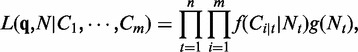
We now demonstrate a model where read coverage will be used as the observed variables for abundance estimation. Assume the sequencing procedure as a random sampling process, in which every read is sampled independently and uniformly from every possible nucleotide in the transcripts (29). For a single transcript t in an ASM, the probability that a read from t falls in e is . Given the total number of reads from t, the number of reads falling in segment e , follows a binomial distribution with parameters and 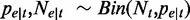. When is sufficiently large, the binomial distribution can be well approximated using a normal distribution with mean and variance 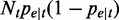, written as . Let r denote the length of a read. The value of represents the read coverage on e contributed by t, , whereas the value of represents the read coverage on t, . Therefore, we have 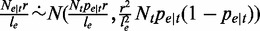, equivalently and

(1)

For a splice junction j, its length is defined to equal the read length r, which is the length of the exonic region, where reads starting in this region can cover the splice junction. The number of spliced reads from t that covers j, still follows the normal distribution in Equation (1).

From Equation (1), and are unbiased for . The variance of varies according to the coverage and the segment length . Dividing the difference between and by , we have the ratio following a normal distribution . Higher coverage and longer segments lead to estimators with smaller variance of the relative deviation from the true transcript coverage, which we demonstrate in the simulated results (Figure 3).

Figure 3.

Evaluation of DiffSplice on simulated data set under different sampling depth. (a) Scatterplot of profile JSD and DiffSplice JSD at different sampling depth. (b) JSD correlation and MSE of path distribution at different sampling depth (from 10 to 100%). (c) MSE of path distribution grouped by different expression quartile. (d) MSE of path distribution grouped by different discriminative length quartile. Within each quartile group, the box plot of the MSE is plotted for every read set (from left to right: the read sets with sampling depth percentile of 10 through 100%).

Estimation of alternative ASM path abundance

Consider an ASM with totally m exonic segments and splice junctions. Assume consists of n alternative transcription paths. The exonic length of a path t is hence given as 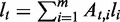, where if path t covers the ith exonic segment and otherwise. Let denote the relative proportions of the alternative paths, with . The probability of a read falling into path t is then written as , with . Assume the number of reads sampled from follows a Poisson distribution with parameter N, where N represents the expression of in the sample accounting for the depth of sequencing and the length of (29). The number of reads sampled from path t, then follows a Poisson distribution with parameter , i.e.

(2)

We hence derive the maximum likelihood estimators for the path proportion, q, and the expected total number of reads in , N. With observed read coverage on every exonic segment and splice junction, the likelihood of q and N is the joint density of through under q and N,

We assume that are mutually independent. The likelihood function can be factorized as:

(3)

where is the density of the exonic/junction coverage distribution in Equation(1), and is the density of the transcript read count distribution in Equation (2). We then use the expectation maximization algorithm to derive the maximum likelihood estimators for q and N (Supplementary Section S2). In addition to estimating transcription path proportions, the expectation maximization algorithm also calculates the expected expression of each transcription path, . Then, the expected expression of sums up the expected expression of all transcription paths in , forming an estimator for the total number of transcript copies passing through .

Estimation of gene expression

Within a gene G, the abundance estimation procedure starts from the minimal ASMs, i.e. the ASMs in the bottom level of the decomposition hierarchy, then propagates toward the top of the hierarchy. During inference within an ASM , all ASMs nested in must have performed the alternative path abundance estimation and hence are treated as single exonic segments, using their estimated expression as the exonic coverage. The estimator for the expression of gene G, is hence the mean expression of all the exonic segments and ASMs that directly constitute G (or in the decomposition hierarchy all the children of G on the first level). This estimator provides a direct measure for the expected total number of transcript copies in gene G in the RNA-seq sample.

Statistical test for differential transcription

Differential expression under different conditions may exhibit in two aspects. At the gene level, the difference in a gene’s expression level measures the change of the total expression of all the transcripts in this gene (‘differential gene expression level’). At the transcript level, the difference in the relative proportion of alternative transcription paths reflects the regulation on the expression of individual transcripts (‘differential gene transcription’). In DiffSplice, we test the two levels of differences separately. Based on the estimators for gene expression level derived in the previous section, we use the same method as proposed in Significance Analysis of Microarrays (SAM) (31) to test for difference in gene expression under different conditions (groups). Then, we extend the method to test for difference in transcription by defining test statistic in terms of divergence between relative expression profiles of alternative paths.

Test statistic for differential gene transcription

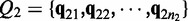The transcript-level expression of a gene is characterized by the relative proportion of the alternative transcription paths in every ASM of this gene. Let and denote two groups of samples. Let and denote the estimated path proportion of an ASM in each sample. Let and denote the mean distributions of the two sample groups.

To select significant differences in transcription, we look for ASMs with significant difference in path distributions between the two groups but consistent path distributions within each group. We use the square root of the Jensen–Shannon divergence (JSD) (32) to quantitate the dissimilarity between two distributions as a real value between 0 and 1 (Supplementary Section S3). We define the between-group difference as the divergence between the group mean distributions,

(4)

The within-group variance of each group is defined as:

(5)

where is the normalization constant.

Abundance estimation on ASMs with low expression often associates with higher unstability. Therefore, we add as a penalty for low expression, based on a logistic function of the averaged estimated expression of the ASM ,

(6)

where adjusts the penalized expression range of low ASM expression (e.g. for penalizing ASMs with estimated expression <∼6 while assigning negligible penalty to ASMs with higher expression) and denotes the largest variance among all ASMs in the data.

Therefore, the relative difference in transcription of an ASM is in the form:

(7)

measuring the extent how the distributions over alternative paths within the ASM consistently differ between the two groups.

Permutation test

An empirical distribution of relative difference can be obtained by calculating test statistics after permuting samples across groups (31). Suppose totally M ASMs are tested for differential transcription. The relative transcriptional difference is calculated for every ASM, and the order statistics are collected, . Under each permutation p, order statistics of relative differences could also be calculated in the same way: . Averaging order statistics from all permutations, we have the expected relative difference in transcription: 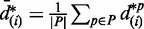for , where P is the set of all permutations and is the number of permutations.

Statistical significance

Significant changes on transcription are concluded based on the extent of disagreement between calculated and expected test statistics. Given a threshold , an ASM with relative transcription difference of is accepted to have significant difference on transcription, if 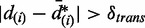. The choice of is monitored by its associated FDR, which we define next.

False discovery rate

At a cutoff of , the quantity of falsely discovered ASMs in each permutation is estimated as the number of ASMs, such that 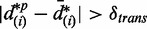. The FDR for differential transcription is hence estimated as the averaged number of falsely discovered ASMs over all permutations, divided by the total number of ASMs.

RESULTS

Experimental results with simulated data sets

The following set of experiments first evaluated the accuracy of DiffSplice on data sets simulated on the entire human transcriptome with varying sampling depth and varying degrees of 5′ or 3′ positional bias. We then compared DiffSplice with the state-of-the art methods, including Cufflinks and FDM, on the simulated data set used by Singh et al. (13).

Simulation of RNA-seq data sets

We developed an in-house simulator to generate two RNA-seq data sets on human transcriptome. In each data set, we generated pairs of RNA-seq samples under various sampling depth or sampling bias. For every sample, the simulator randomly generates relative expression profiles for the transcripts, based on the user-provided human transcriptome annotation. A number of complementary DNA (cDNA) molecules are then assigned to every transcript according to its expression level and the size of the data set. A cDNA library is hence constructed through steps as amplification and size selection, and RNA-seq reads are sampled from the cDNA library.

For every pair of samples, we first calculate their transcriptional difference at each ASM based on the transcript annotation and expression profiles used in generating the RNA-seq data, referred to as the ‘profile JSD’. The difference in ASM estimated by DiffSplice directly from the RNA-seq reads is referred to as the ‘DiffSplice JSD’. The profile JSD reflects the ground truth difference in each ASM, whereas the DiffSplice JSD is an estimation from sampled reads. We calculate the Pearson correlation between the two as a measure for the accuracy of the estimated difference, denoted by the ‘JSD correlation’. We also consider a complementary measure for every ASM, the mean squared error (MSE), which calculates the error of the estimated path distribution from the distribution in the expression profile. We average the MSE from both samples in a pair-wise comparison, which is denoted as the ‘MSE of path distribution’.

Human transcriptome under varying sampling depth

We first study the effect of the sampling depth on the abundance estimation. We simulated 10 pairs of samples on human transcriptome, from 10 M (10%) reads to 100 M (100%) reads. For each sample, 2 × 75 bp PER with average insert size of 100 bp were generated. Genes with averaged read coverage per base >10 were picked to compare the difference by profile and the difference derived by DiffSplice. Figure 3a shows the scatterplots of profile JSD against JSD estimated by ASM in read sets of 10 M (10%), 40 M (40%), 70 M (70%) and 100 M (100%) reads. The data with relatively lower sampling depth (e.g. depth = 10%) show less points than the data with higher sampling depth because it covers less ASMs. However, all sets have most points close to the diagonal, indicating minimal deviation between profile JSD and estimated JSD. The correlations range from 0.85 to 0.88 (Figure 3b). Higher JSD correlation is achieved by increasing the sampling depth, while the MSE of path distribution also decreases. Figure 3c separates all ASMs into four quartile groups according to their expression level and compares the distribution of MSE in each group. ASMs with higher expression separate randomness of read sampling and result in more stable estimates. As expected, the upper two quartiles exhibit better estimates than the lower two quartiles, in terms of both smaller mean and lower variance.

Besides the expression of the ASMs, the variance of the abundance estimator is also related to the ‘discriminative length’, the length of the exonic regions that are specific to a path in an ASM. Figure 3d groups all ASMs into four quartiles according to the discriminative length. ASMs with larger discriminative length are also expected to be more robust to random sampling errors and have higher accuracy on discriminating difference between path distributions. The lowest quartile has slightly higher MSE than the rest 75% ASMs. In contrast, the MSE sharply decreases in all groups, emphasizing the impact of sampling depth over discriminative length in improving abundance estimation accuracy.

Human transcriptome under varying sampling bias

Methods that estimate transcript abundance are typically designed under the assumption that the RNA-seq fragments are sampled independently, and the sampling position is uniformly distributed along the transcript from which the fragments originate. The transcript inference and thereafter the evaluation of differential expression may be altered if sampling bias is introduced by sample preparation protocols. Two types of sampling bias are commonly observed in RNA-seq data, namely, position-specific bias and sequence-specific bias (30,33–35).

We specifically looked at 3′ bias that is a typical position-specific bias. To simulate the data, we introduce a parameter β to represent the degree of sampling bias, such that equals to the ratio of the sampling probability at the last base in the 3′-end of a transcript over the sampling probability at the first base in the 5′ end of the transcript. The sampling probability at a middle bases t is then calculated as a linear interpolation, , where denotes the distance from the base t to the 5′ end of the transcript, and l denotes the length of the transcript.

We simulated 11 read sets on human transcriptome under from 0 to 2.0. Figure 4a shows the scatterplots of the profile JSD against the DiffSplice JSD in read sets under no bias and bias of 0.6, 1.2 and 1.8. All sets have most estimated JSD close to profile JSD, with no significant effect of sampling bias. This is consistent with Figure 4b, where the correlations range from 0.878 to 0.887. The MSE is slightly lower when no bias is introduced but remains roughly unchanged as increases, indicating the robustness against altered sampling distribution of the alternative path estimation by DiffSplice. In Figure 4c and d, ASMs are again grouped into quartile groups according to their expression level and discriminative length. Although the expression level still dominates the accuracy of path abundance estimation, no significant effect of sampling bias is observed in all groups.

Figure 4.

Evaluation of DiffSplice on simulated data set in the presence of position-specific sampling bias. (a) Scatterplot of profile JSD and DiffSplice JSD at different β. (b) JSD correlation and MSE of path distribution at different β (from 0 to 2). (c) MSE of path distribution grouped by different expression quartile. (d) MSE of path distribution grouped by different discriminative length quartile. Within each quartile group, the box plot of the MSE is plotted for every read set (from left to right: the read sets with β of 0 through 2).

Differential transcription between two groups of samples

We further applied our method to the two simulated data sets used in the evaluation of FDM (13). More than 2100 genes with at least two transcripts were simulated in the two tissues, each tissue having four replicates. The square root of the JSD between transcript profiles of the two tissues was calculated for each gene to suggest the ‘true’ transcriptional difference. The coverage of each gene was calculated to measure the expression level. Genes with coverage >1 were chosen for comparison. In addition to DiffSplice, three other methods (FDM, Cuffdiff with annotation and Cuffdiff without annotation) were also applied on this data set. FDM was run using no transcriptome annotation information. With FDR <0.01, DiffSplice reported 887 genes with significant difference on transcription. At confidence level of 0.05, FDM, Cuffdiff with annotation and Cuffdiff without annotation reported 722, 931 and 530 differentially transcribed genes, respectively.

Figure 5a–d plot the genes coordinated by the square root of its profile JSD and the logarithm of its coverage. The genes with significant differences on transcription identified by each method are represented by red dots. The genes with insignificant differences are represented by blue circles. Along the x-axis, the majority of the significantly differentiated genes identified by DiffSplice have large profile JSD (square root of profile JSD > 0.2), showing that DiffSplice correctly captures transcriptional divergences between the two tissues. Along the y-axis, the most significant genes identified by DiffSplice have relatively high coverage. This follows the fact that differences present in highly expressed genes are less likely to occur randomly or be introduced by sampling error and hence have higher confidence. We calculate the sensitivity of all four methods at genes that have large profile difference, as well as high expression, for example, the region with square root of profile JSD >0.25 and coverage >5. Among the 548 genes in that region (the up-right part), DiffSplice identified 506 genes as significant differences, with a sensitivity of 92% (506 of 548). This sensitivity is 10 percentage points higher than those of FDM (80% or 437 of 548) and Cuffdiff with annotation (81% or 443 of 548), and 30 percentage points higher than that of Cuffdiff without annotation (58% or 316 of 548). To assess the rate of false positives, we further calculate the precision for every method, defined as the proportion of the true significant genes called by each method in all the significant genes called by the method. The precision of DiffSplice (57%) is close to those of FDM (61%) and Cuffdiff without annotation (60%) and is 9 percentage points higher than that of Cuffdiff with annotation (48%).

Figure 5.

Comparison among DiffSplice, FDM, and Cufflinks on simulated data set of human transcriptome. (a–d) Scatterplot of coverage against profile JSD for results of (a) DiffSplice, (b) FDM, (c) Cufflinks with annotation and (d) Cufflinks without annotation, respectively. The majority of the differentially transcribed genes identified by DiffSplice (plotted as red dots) have square root of profile JSD > 0.2 and log coverage >0.5. Setting the genes with square root of profile JSD > 0.25 and coverage >5 to have significant difference in profile, DiffSplice achieves a sensitivity of 92%, higher than those of FDM (80%), Cuffdiff with annotation (81%) and Cuffdiff without annotation (58%). (e–h) Scatterplot of variance against profile JSD for results of (e) DiffSplice, (f) FDM, (g) Cufflinks with annotation and (h) Cufflinks without annotation, respectively. Most of the differentially transcribed genes identified by DiffSplice (plotted as red dots) have variance <0.1. Setting the genes with square root of profile JSD > 0.25 and variance <0.1 to have significant difference in profile, DiffSplice reaches a sensitivity of 89%, higher than those of FDM (74%), Cuffdiff with annotation (80%) and Cuffdiff without annotation (40%).

The test statistic of DiffSplice also takes into account the variance of alternative path distributions among the replicates in each group. Figure 5e–h plot the genes coordinated by the square root of its profile JSD and the within-tissue variance of its transcript profile. The genes with significant or insignificant differences are still represented by red dots and blue circles, respectively. Almost all significant genes identified by DiffSplice have low profile variance compared with profile divergence. We also calculate the sensitivity of all four methods at genes that have large profile difference, as well as small within-tissue variance, for example, the region with square root of profile JSD > 0.25 and variance <0.1. Among the 952 genes in that region (the bottom-right part), DiffSplice identified 849 genes as significant differences, with a sensitivity of 89% (849 of 952). This sensitivity is 15 percentage points higher than that of FDM (74% or 705 of 952), nearly 10 percentage points higher than Cuffdiff with annotation (80% or 764 of 952), and 40 percentage points higher than that of Cuffdiff without annotation (49% or 462 of 952). DiffSplice also has a precision (96%) close to FDM (98%) and clearly higher than Cuffdiff with annotation (82%) and Cuffdiff without annotation (87%).

Experimental results with real data sets

Lung differentiation data set

The human lung airway epithelium lies on the lung–environment interphase, serving as the important physical barrier against invading pathogens. It is composed of various cell types, including ciliated cells, mucus-secretory goblet cells and basal cells, differentiated from specialized cells in varying numbers. We hypothesized that genes expression changes, including the differential expression of alternative spliced isoforms, are key in the mucociliary cell differentiation and function. Thus, we have sequenced mRNAs from primary human bronchial cells at the early (Day 3) and late (Day 35) differentiation stages, respectively, by high-throughput sequencing. Three biological replicates were used in each group (Day 3 versus Day 35). Following the manufacturer’s instruction, mRNA libraries were made for each sample, and ∼28 million 76-bp single-end reads were generated from each sample for analysis. The biological findings from this experiment will be presented in another report.

The RNA-seq reads were mapped by MapSplice 1.15.1 (18) to the human reference genome (hg19). About 94% were mapped for each sample. DiffSplice was then performed on these read alignments. Cufflinks + Cuffdiff pipeline (version 1.1.0 with bias correction) was also run on the same read alignments with results both using and not using transcriptome annotation generated for comparison.

As shown in Figure 6a, DiffSplice identified 2077 genes that have differential gene expression level between Day 3 and Day 35 at FDR < 0.01 and requiring the fold change of >2 (up-regulated) or < (down-regulated). This number is similar to the results obtained from the SAM analysis (31). At Day 35, 1429 genes were tested to have significantly higher expression level than at Day 3, whereas 648 genes were tested to have significantly lower expression level than at Day 3. This observation has indicated active metabolism biogenesis process occurring during the airway epithelium differentiation. At FDR < 0.01, DiffSplice also identified 498 genes exhibiting significant differentiation on alternative transcription. Among them, 109 genes had significantly altered overall gene expression, whereas the rest 389 genes were differentially transcribed while their total gene expression remains at the same level. We randomly selected genes with the inter-group square root of JSD > 0.3 for qRT-PCR validation (Supplementary Figure S6). The expression profiles of two validated genes TMC5 and LMO7 are included in Figure 7 and Supplementary Figure S7.

Figure 6.

Comparison between DiffSplice and Cufflinks on the lung differentiation data set. (a) Differential expression discovered by DiffSplice using MapSplice alignment without annotation. (b) Comparison among differentially transcribed genes discovered by DiffSplice, Cufflinks with annotation and Cufflinks without annotation. (c) Percentage of significant genes with differential transcription against number of transcripts. (d) Number of significant genes with differential transcription against percentage of samples with gene coverage <3 in each group. (e) Differential transcription in gene PI4KB, identified by DiffSplice but missed by Cufflinks without annotation.

Figure 7.

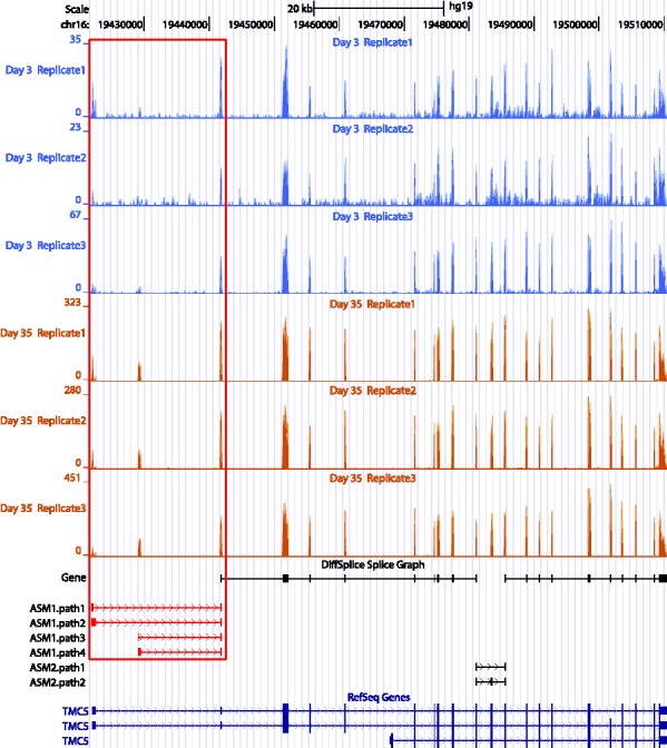
Alternative transcription start sites identified by DiffSplice in gene TMC5. The relative expression of isoform passing ASM1.path4 increased significantly from Day 3 to Day 35. The change has been validated by qRT-PCR experiment (Supplementary Figure S6). Meanwhile, the overall gene expression level also significantly increased with a fold change of ∼11.

We compared the differentially transcribed genes identified by DiffSplice and Cufflinks + Cuffdiff. Cufflinks + Cuffdiff with annotation reported >7000 genes that have significant differential transcription events between Day 3 and Day 35, whereas Cufflinks + Cuffdiff without annotation only reported ∼3000 genes. In comparison, DiffSplice reported 498 genes with 77 and 54% overlapped with results of Cufflinks + Cuffdiff with and without annotation, respectively. The result is shown as Venn diagram in Figure 6b. Next, we detail the major issues from the investigation of the discrepancy.

Effect of transcription complexity

In general, genes with larger number of isoforms tend to have more splicing events, and therefore have a higher chance to be differentially transcribed. Nevertheless, having the majority of the genes detected to be significantly different indicates a high level of false positive discovery rate. In Figure 6c, we divided genes into groups according to the number of isoforms and plotted the percentage of genes detected to be significant as a function of the number of isoforms. As high as 80% of genes with more than five isoforms were identified as having significant differential transcription by Cufflinks + Cuffdiff with annotation, and ∼50–75% of genes with more than five known isoforms were identified as significant by Cufflinks + Cuffdiff without annotation. The decreased number of significance called by Cuffdiff without annotation correlates with the typically lesser number of reconstructed transcripts in a gene than the number of annotated transcripts. In contrast, the percentage of genes detected to be differentially transcribed is typically <10% with DiffSplice, with a trend of raising percentage as transcriptome complexity increases.

Transcripts in genes with high transcription complexity are difficult to infer and quantify, requiring a high read coverage to be reliable. Inaccurate transcript inference and/or quantification may not only lead to false positive discovery of the differentially transcribed genes but also may miss genes that are truly differentially transcribed. In gene PI4KB, DiffSplice discovered two ASMs, as shown in Figure 6e. The first ASM starts from the fourth exon (from the 5′ end) and ends at the sixth exon, alternatively excluding or including the fifth exon. The second ASM spans from the first exons to the fourth exon, alternatively transcribing the second and the third exon. The first ASM was tested to have significant difference in transcription by DiffSplice, which had significantly higher exon-skipping ratios at Day 3. Without annotation, Cufflinks failed to point out this difference. Cufflinks took the combination of the two alternative splicing events and assembled seven transcripts, containing three spurious transcripts compared with RefSeq annotation. In addition to the inconsistency in assembled transcripts, the estimated transcript abundance by Cufflinks did not reflect the shift on expression. Combining the transcripts that included the fifth exon (TCONS_00003827, 00003831 and 00003833), the total expression of the three transcripts was 8.63 at Day 3 and 9.27 at Day 35 [in (Reads Per Kilobase per Million mapped reads (RPKM)], which did not match the observed increase on the expression of the fifth exon. Also, the overall expression of all the seven assembled transcripts fell from 18.8 (Day 3) to 16.6 (Day 35), which did not match the observation that the overall expression was actually higher in Day 35. In gene TMC5, DiffSplice discovered an alternative transcription start event with four alternative start sites and an exon-skipping event (Figure 7). The alternative start event was tested to have significantly higher abundance of the path ASM1.path4 at Day 35 (48.9%) than Day 3 (14.7%). This finding was consistent with the result of qRT-PCR experiment that the alternative start site corresponding to ASM1.path4 had its abundance at Day 35 at least twice as high as its abundance at Day 3. This gene was also found having differential expression level, with its expression at Day 35 >10 times higher than that at Day 3.

Effect of coverage and variance in replicates

When determining differential transcription, read coverage needs to be sufficiently high to make a reliable inference on the transcript expression. In Figure 6d, we plot the number of genes that were called to be significantly different in transcription against the number of samples with exceptionally low expression (e.g. gene coverage <3). The three methods in comparison detect similar percentage of significant genes when the majority of the samples are well expressed. However, Cufflinks + Cuffdiff calls hundreds of genes as significantly differentiated when almost all samples in a group are barely expressed at all.

Besides, Figure 6d also indirectly shows high within-group variance among replicates. In testing of differential expressed or transcribed genes, the variance among samples within the same group is expected to be low and should be well controlled. More than three of nine replicates in one of the comparison groups had extremely low coverage in 269 genes detected by Cufflinks + Cuffdiff with annotation and 128 genes detected by Cufflinks + Cuffdiff without annotation, demonstrating high within-group variance of these genes.

Novel alternative splicing

As DiffSplice takes only RNA-seq read alignments as input and relies on no annotation, it captures splicing events that are only relevant to the given mRNA samples and has the capability of discovering novel alternative transcripts. We categorize an ASM detected by DiffSplice into four types: the ASM exactly matches an annotated ASM; the ASM is a subgraph of an annotated ASM; the ASM partially overlaps with an annotated ASM and the ASM is not found in the annotation. The histogram of each category at varying coverage is shown in Figure 8a. The ASMs detected by DiffSplice show high consistency with those generated from known annotation. Among the 5556 ASMs found be DiffSplice, 2426 ASMs matched an annotated ASM, and 2219 ASMs were subsets of annotated ASMs. Besides the alternative splicing events present in annotation, we found 174 ASMs with novel paths added to annotated ASMs and 736 novel ASMs. For example, we discovered a novel exon in gene STRA13, located between the second and the third exon in the RefSeq annotation (Figure 8b). This exon was discovered as differentially skipped between Day 3 (50% skipping ratio) and Day 35 (30% skipping ratio). Because the exon-skipping event in STRA13 is not present in the transcriptome annotation, Cufflinks with annotation did not capture the difference. Cufflinks without annotation falsely initiated a transcript from the third annotated exon and did not detect the event either.

Figure 8.

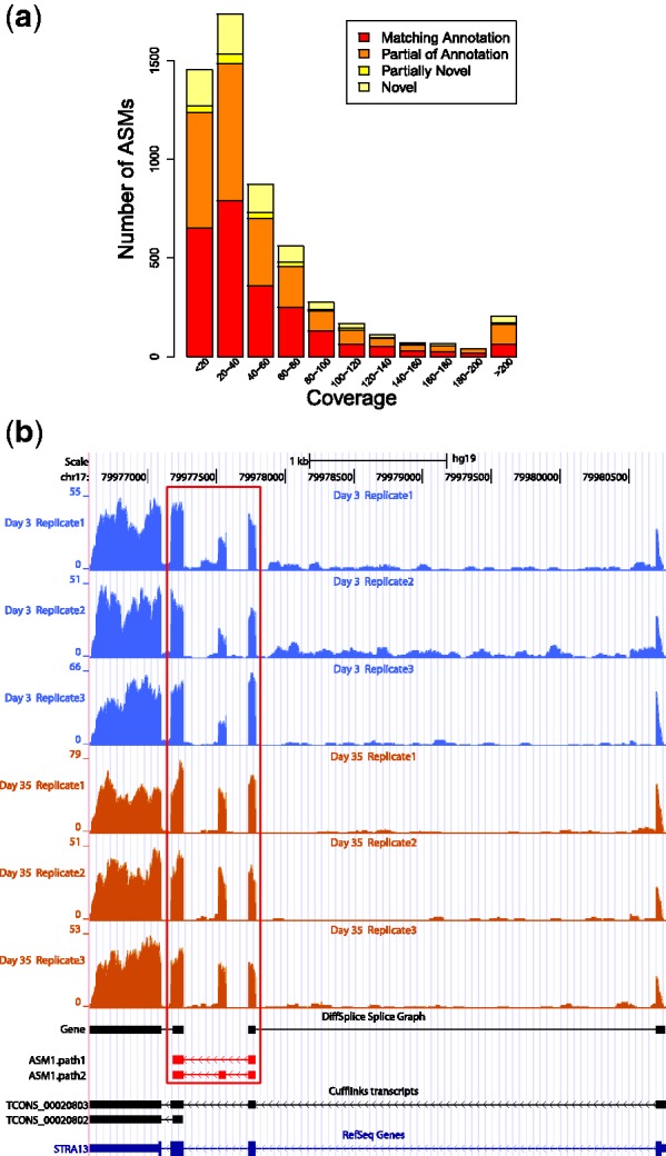
DiffSplice discovers alternative splicing variants present in the data. (a) Number of ASMs discovered by DiffSplice at different expression level. Besides ∼2400 ASMs that exactly match annotated ASMs, DiffSplice discovered >2000 ASMs, where only subsets of annotated splicing variants were present, nearly 200 ASMs with novel splicing variants added to annotated alternative splicing events and >700 ASMs that were completely new to the annotation. (b) Novel alternative splicing in gene STRA13, identified by DiffSplice but missed by Cufflinks both with and without annotation. DiffSplice discovered a novel exon in the annotated intron region between the second and the third exon of STRA13. Splice junctions evidenced that the exon was alternatively excluded (path 1) or included (path 2) in transcripts of this gene, and the skipping ratio was tested to have significantly decreased from Day 3 to Day 35.

Breast cancer data set

We further applied DiffSplice to the RNA-seq data sets generated from two breast cancer cell lines, MCF7 and SUM102 (13). Each cell line group comprises of four technical replicates, and ∼80 million 100-bp single-ended reads were sequenced for each replicate. FDM was originally applied to these data sets to detect genes that might have differentially transcribed without usage of transcriptome annotation information (13). At FDR < 0.01, DiffSplice identified 6103 genes with significant difference on expression level and 2507 genes with significant difference on transcription between the two cell lines, including 1353 genes with both differences. For genes that were differentially transcribed, DiffSplice had 955 (38.1%) shared with those discovered by FDM (Supplementary Section S6.3).

DiffSplice successfully identified the two genes CD46 (Figure 9a) and NPC2 (Figure 9b) that were originally validated by qRT-PCR in FDM article. However, unlike FDM, DiffSplice directly pinpoints the location of alternative splicing events that are differentially expressed, consistently with those chosen for the qRT-PCR validation. For example, in the exon-skipping event found in CD46 (Figure 9a), the averaged estimated proportion of the path that included the 13th exon (chromosome1:207963598–207963690) was 34.7% in the SUM102 group and 13.9% in the MCF7 group. This result was consistent with the observation in the qRT-PCR experiment that the skipped exon had >2-fold higher expression level in SUM102 than in MCF7. In gene NPC2, DiffSplice discovered two alternative splicing events, one nested within the other (Figure 9b). The intron retention occurs between the last two exons was found present primarily only in MCF7 samples. This ASM was further nested in a larger exon-skipping event spanning the last three exons, where the second exon was alternatively spliced with a significantly lower skipping ratio in SUM102 samples. The first intron-retention event was picked for qRT-PCR validation. The averaged estimated proportion of the path that retained the intron (chromosome14:74946992–74947388) was 0.5% in the SUM102 group and 17.9% in the MCF7 group, consistent with the experimental observation that the retained intron had at least 10-fold higher expression level in MCF7 than in SUM102.

Figure 9.

DiffSplice on the breast cancer data set. (a) Differential transcription on skipped exon in gene CD46 identified by DiffSplice. DiffSplice discovered two ASMs in this gene. The second ASM that alternatively skipped the 13th exon was tested to have significantly higher skipping ratio in MCF7 samples. This transcriptional difference has been validated by qRT-PCR experiment. (b) Differential transcription on retained intron in gene NPC2 identified by DiffSplice. The exon-skipping event spanning the left three exons was tested to have significantly higher skipping ratio in MCF7 samples. The nested intron retention in the left two exons was also tested to have significantly higher ratio of retaining the intron in MCF7 samples. The differential transcription in the intron-retention event has been validated by qRT-PCR experiment.

Besides alternatives spliced events, DiffSplice can be generalized to detect structural variations whose presence is different across two comparison groups. Forty-two genes were detected to have a small insertion/deletion that varies between MCF7 and SUM102. As shown in Figure 10, a 19-bp novel deletion was discovered in the last exon of gene REEP4. The averaged estimated proportion of the path that included the deletion was >99.2% in SUM102 samples. The estimated proportion of the deletion fell to 49.9% as turning to MCF7 group. We directly resequenced the genomic DNA and the cDNA derived from the mRNA of the cell lines and validated this novel deletion. These deletions evidenced the genomic variation present in cancer cell lines and may contribute to prognostic differences together with other differential expression events.

Figure 10.

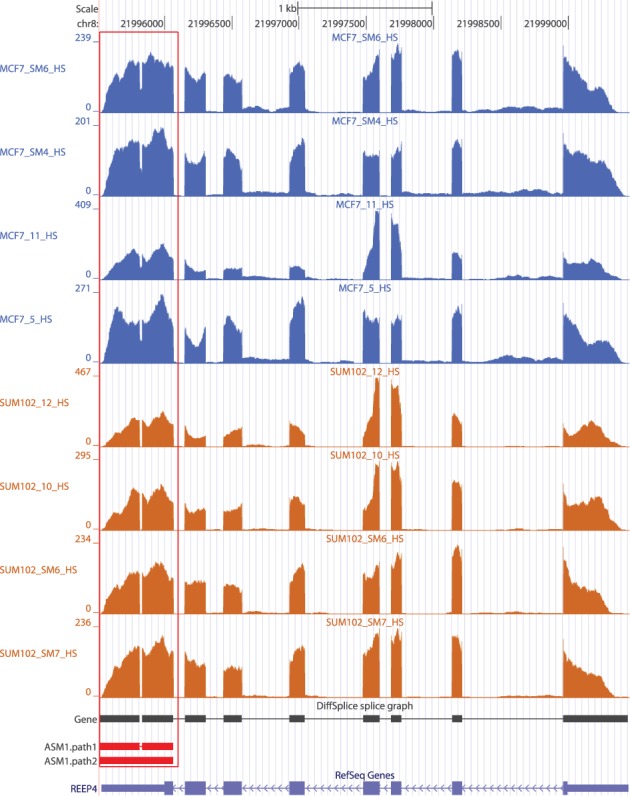
A novel deletion in gene REEP4 found differentially transcribed between SUM102 and MCF7 by DiffSplice. In SUM102, 19 bp were deleted in almost all transcripts compared with the reference genome. In MCF7, the deletion was only present in approximately half of the transcripts. This novel deletion has been validated through resequencing.

DISCUSSION

We present an ab initio method for the detection of alternative splicing isoforms that are differentially expressed under different conditions using high-throughput RNA-seq reads. Our approach does not rely on the information of full-length transcripts of any sort, either from annotation or from computational inference. Instead, the information carried by the RNA-seq read alignment is summarized and condensed using a concise splice graph. The splice graph is then decomposed into a collection of ASMs, where more accurate abundance estimation and differential testing will be performed. Our approach directly localizes where differential splicing occurs, making it easier to identify exons involved in alternative transcription.

In comparison with differential analysis based on transcript quantification such as Cufflinks, DiffSplice isolates the divergences in alternatively spliced regions from the overall gene structure and alleviates potential false positives due to high complexity in transcription (e.g. large number of transcripts), as shown in the lung differentiation data set. Furthermore, DiffSplice is data driven. It extracts information directly from RNA-seq read alignment and is capable of identifying alternative splicing events involving novel transcripts such as novel exons and novel splicing events. More than 100 novel ASMs were discovered in the human lung cell transcriptome, which might be potentially ignored by the methods using annotated splicing features. In addition to alternative splicing events, the identification of ASMs has been further generalized to capture structural variations such as insertions and deletions. The 42 differentially transcribed insertion/deletion events discovered in the breast cancer data set suggest possible cell line-specific regulations by genomic aberrations.

To a biologist used to thinking about alternative splicing as a collection of RNA isoforms, ASM highlights the region(s) of a gene that vary among isoforms. Ultimately, the biologist needs to know how differences among isoforms result in a change in the biological activity of the protein they encode. Investigation of the functional and structural consequences of the alternate exons may reveal what is occurring in genes with ASMs (Supplementary Section S4). Do the exons in an ASM add or remove a known motif? Does that motif require changes in another part of the protein that is reflected in the other ASM? Are the conserved regions the same among samples? Do nested ASMs correspond to hypervariable regions of the protein? In short, careful annotation of an ASM will typically reveal as much as an inferred isoform with little to no risk of an inaccurate reconstruction. The detection and analysis of these local events also can be significant in practice, as suggested by the usage of existing methods. For example, MISO (15) and MATS (17) work entirely on small (non-nested) manually curated ASMs, and have been used by researchers studying alternative splicing. Our method substantially generalizes the analysis and automatically detects the alternative splicing events based on only read alignments.

We use the average read coverage over an exonic region instead of read count at each base as the observed expression. This approach smooths the sampling distribution that might be perturbed during cDNA library preparation by sampling bias, e.g. the sequence-specific bias (33,35). The abundance estimation procedure further incorporates the observed coverage around the alternatively spliced regions on both exons and exon–exon junctions, to improve the quantification accuracy of the transcription flow. As demonstrated through the simulations, this decomposition mechanism in DiffSplice naturally alleviates the sampling bias associated with the position in transcripts (30,33–35).

DiffSplice estimates the relative proportion of alternative transcription flows in every ASM and calculates the JSD to quantify the difference in transcription between samples. Although the relative proportion encodes the distribution of transcripts, it ignores information such as the absolute expression level of every isoform in each sample, which may carry statistical importance for assessment of, e.g. the confidence of the estimated transcript expression. Therefore, new tests for differential transcription may take account of the expression level of transcripts after proper normalization among samples.

DiffSplice is freely available to the academic research community and can be downloaded at http://www.netlab.uky.edu/p/bioinfo/DiffSplice. The software takes the RNA-seq alignment files in standard SAM format as input and generates ASMs in gtf format. When uploaded to the UCSC genome browser, the ASMs with significant differences across sample groups with a given FDR are shown as highlighted tracks.

SUPPLEMENTARY DATA

Supplementary Data are available at NAR Online: Supplementary Figures 1–13, Supplementary Methods and Supplementary References [36–38].

FUNDING

US National Institutes of Health [R01-HG006272 to J.F.P and J.L.]; US National Science Foundation [EF-0850237 to J.L. and J.F.P.]. Additional support was provided by NSF Career award [IIS-1054631 to J.L.]; National Institutes of Health grants [RC1-HL100108 to D.N.H., S.M.H. and S.H.R., AA017376 to L.M., U24-CA143848 and 3U24-CA143848-02S1 to D.N.H., R01-CA149569-03 to Y.L.]; UNC University Cancer Research Fund (to C.J. and L.M.). Funding for open access charge: NIH [R01-HG006272].

Conflict of interest statement. None declared.

REFERENCES

- 1.Sultan M, Schulz M, Richard H, Magen A, Klingenhoff A, Scherf M, Seifert M, Borodina T, Soldatov A, Parkhomchuk D, et al. A global view of gene activity and alternative splicing by deep sequencing of the human transcriptome. Science. 2008;321:956–960. doi: 10.1126/science.1160342. [DOI] [PubMed] [Google Scholar]
- 2.Wang E, Sandberg R, Luo S, Khrebtukova I, Zhang L, Mayr C, Kingsmore S, Schroth G, Burge C. Alternative isoform regulation in human tissue transcriptomes. Nature. 2008;456:470–476. doi: 10.1038/nature07509. [DOI] [PMC free article] [PubMed] [Google Scholar]
- 3.Pan Q, Shai O, Lee L, Frey B, Blencowe B. Deep surveying of alternative splicing complexity in the human transcriptome by high-throughput sequencing. Nat. Genet. 2008;40:1413–1415. doi: 10.1038/ng.259. [DOI] [PubMed] [Google Scholar]
- 4.Kwan T, Benovoy D, Dias C, Gurd S, Provencher C, Beaulieu P, Hudson T, Sladek R, Majewski J. Genome-wide analysis of transcript isoform variation in humans. Nat. Genet. 2008;40:225–231. doi: 10.1038/ng.2007.57. [DOI] [PubMed] [Google Scholar]
- 5.Wang G, Cooper T. Splicing in disease: disruption of the splicing code and the decoding machinery. Nat. Rev. Genet. 2007;8:749–761. doi: 10.1038/nrg2164. [DOI] [PubMed] [Google Scholar]
- 6.Trapnell C, Williams B, Pertea G, Mortazavi A, Kwan G, van Baren M, Salzberg S, Wold B, Pachter L. Transcript assembly and quantification by RNA-Seq reveals unannotated transcripts and isoform switching during cell differentiation. Nat. Biotechnol. 2010;28:511–515. doi: 10.1038/nbt.1621. [DOI] [PMC free article] [PubMed] [Google Scholar]
- 7.Clark T, Sugnet C, Ares M. Genomewide analysis of mRNA processing in yeast using splicing-specific microarrays. Science. 2002;296:907–910. doi: 10.1126/science.1069415. [DOI] [PubMed] [Google Scholar]
- 8.Okoniewski M, Miller C. Comprehensive analysis of affymetrix exon arrays using bioconductor. PLoS Comput. Biol. 2008;4:e6. doi: 10.1371/journal.pcbi.0040006. [DOI] [PMC free article] [PubMed] [Google Scholar]
- 9.Xi L, Feber A, Gupta V, Wu M, Bergemann A, Landreneau R, Litle V, Pennathur A, Luketich J, Godfrey T. Whole genome exon arrays identify differential expression of alternatively spliced, cancer-related genes in lung cancer. Nucleic Acids Res. 2008;36:6535–6547. doi: 10.1093/nar/gkn697. [DOI] [PMC free article] [PubMed] [Google Scholar]
- 10.Wang Z, Gerstein M, Snyder M. RNA-Seq: a revolutionary tool for transcriptomics. Nat. Rev. Genet. 2009;10:57–63. doi: 10.1038/nrg2484. [DOI] [PMC free article] [PubMed] [Google Scholar]
- 11.Huang Y, Hu Y, Jones C, MacLeod J, Chiang D, Liu Y, Prins J, Liu J. A robust method for transcript quantification with RNA-seq data. 16th Annual International Conference on Research in Computational Molecular Biology (RECOMB) 2012;7262:127–147. doi: 10.1089/cmb.2012.0230. Barcelona, Spain. [DOI] [PMC free article] [PubMed] [Google Scholar]
- 12.Stegle O, Drewe P, Bohnert R, Borgwardt K, Rätsch G. Nature Precedings. 2010. Statistical tests for detecting differential RNA-transcript expression from read counts. doi:10.1038/npre.2010.4437.1. [Google Scholar]
- 13.Singh D, Orellana C, Hu Y, Jones C, Liu Y, Chiang D, Liu J, Prins J. FDM: a graph-based statistical method to detect differential transcription using RNA-seq data. Bioinformatics. 2011;27:2633–2640. doi: 10.1093/bioinformatics/btr458. [DOI] [PMC free article] [PubMed] [Google Scholar]
- 14.Griffith M, Griffith O, Mwenifumbo J, Goya R, Morrissy A, Morin RD, Corbett R, Tang M, Hou Y-C, Pugh T, et al. Alternative expression analysis by RNA sequencing. Nat. Methods. 2010;7:843–847. doi: 10.1038/nmeth.1503. [DOI] [PubMed] [Google Scholar]
- 15.Katz Y, Wang E, Airoldi E, Burge C. Analysis and design of RNA sequencing experiments for identifying isoform regulation. Nat. Methods. 2010;7:1009–1015. doi: 10.1038/nmeth.1528. [DOI] [PMC free article] [PubMed] [Google Scholar]
- 16.Wu J, Akerman M, Sun S, McCombie W, Krainer A, Zhang M. SpliceTrap: a method to quantify alternative splicing under single cellular conditions. Bioinformatics. 2011;27:3010–3016. doi: 10.1093/bioinformatics/btr508. [DOI] [PMC free article] [PubMed] [Google Scholar]
- 17.Shen S, Park J, Huang J, Dittmar KA, Lu Z, Zhou Q, Carstens RP, Xing Y. MATS: a Bayesian framework for flexible detection of differential alternative splicing from RNA-Seq data. Nucleic Acids Res. 2012;40:e61. doi: 10.1093/nar/gkr1291. [DOI] [PMC free article] [PubMed] [Google Scholar]
- 18.Wang K, Singh D, Zeng Z, Huang Y, Coleman S, Savich G, He X, Mieczkowski P, Grimm S, Perou C, et al. MapSplice: accurate mapping of RNA-seq reads for splice junction discovery. Nucleic Acids Res. 2010;38:178. doi: 10.1093/nar/gkq622. [DOI] [PMC free article] [PubMed] [Google Scholar]
- 19.Hu Y, Wang K, He X, Chiang D, Prins J, Liu J. A probabilistic framework for aligning paired-end RNA-seq data. Bioinformatics. 2010;26:1950–1957. doi: 10.1093/bioinformatics/btq336. [DOI] [PMC free article] [PubMed] [Google Scholar]
- 20.Heber S, Alekseyev M, Sze S, Tang H, Pevzner P. Splicing graphs and EST assembly problem. Bioinformatics. 2002;18(Suppl. 1):S181–S188. doi: 10.1093/bioinformatics/18.suppl_1.s181. [DOI] [PubMed] [Google Scholar]
- 21.Birol I, Jackman S, Nielsen C, Qian J, Varhol R, Stazyk G, Morin R, Zhao Y, Hirst M, Schein J, et al. De novo transcriptome assembly with ABySS. Bioinformatics. 2009;25:2872–2877. doi: 10.1093/bioinformatics/btp367. [DOI] [PubMed] [Google Scholar]
- 22.Grabherr M, Haas B, Yassour M, Levin J, Thompson D, Amit I, Adiconis X, Fan L, Raychowdhury R, Zeng Q, et al. Full-length transcriptome assembly from RNA-Seq data without a reference genome. Nat. Biotechnol. 2011;29:644–652. doi: 10.1038/nbt.1883. [DOI] [PMC free article] [PubMed] [Google Scholar]
- 23.Li R, Zhu H, Ruan J, Qian W, Fang X, Shi Z, Li Y, Li S, Shan G, Kristiansen K, et al. De novo assembly of human genomes with massively parallel short read sequencing. Genome Res. 2010;20:265–272. doi: 10.1101/gr.097261.109. [DOI] [PMC free article] [PubMed] [Google Scholar]
- 24.Trapnell C, Pachter L, Salzberg S. TopHat: discovering splice junctions with RNA-Seq. Bioinformatics. 2009;25:1105–1111. doi: 10.1093/bioinformatics/btp120. [DOI] [PMC free article] [PubMed] [Google Scholar]
- 25.Au K, Jiang H, Lin L, Xing Y, Wong W. Detection of splice junctions from paired-end RNA-seq data by SpliceMap. Nucleic Acids Res. 2010;38:4570–4578. doi: 10.1093/nar/gkq211. [DOI] [PMC free article] [PubMed] [Google Scholar]
- 26.Ferrante J, Ottenstein K, Warren J. The program dependence graph and its use in optimization. ACM Trans. Program. Lang. Syst. 1987;9:319–349. [Google Scholar]
- 27.Pingali K, Bilardi G. Optimal control dependence computation and the Roman chariots problem. ACM Trans. Program. Lang. Syst. 1997;19:462–491. [Google Scholar]
- 28.Buchsbaum A, Kaplan H, Rogers A, Westbrook J. A new, simpler linear-time dominators algorithm. ACM Trans. Program. Lang. Syst. 1998;20:1265–1296. [Google Scholar]
- 29.Jiang H, Wong W. Statistical inference for isoform expression in RNA-Seq. Bioinformatics. 2009;25:1026–1032. doi: 10.1093/bioinformatics/btp113. [DOI] [PMC free article] [PubMed] [Google Scholar]
- 30.Srivastava S, Chen L. A two-parameter generalized Poisson model to improve the analysis of RNA-seq data. Nucleic Acids Res. 2010;38:e170. doi: 10.1093/nar/gkq670. [DOI] [PMC free article] [PubMed] [Google Scholar]
- 31.Tusher V, Tibshirani R, Chu G. Significance analysis of microarrays applied to the ionizing radiation response. Proc. Natl Acad. Sci. USA. 2001;98:5116–5121. doi: 10.1073/pnas.091062498. [DOI] [PMC free article] [PubMed] [Google Scholar]
- 32.Lin J. Divergence measures based on the shannon entropy. IEEE Trans. Inf. Theory. 1991;37:145–151. doi:10.1109/18.61115. [Google Scholar]
- 33.Bohnert R, Rätsch G. rQuant.web: a tool for RNA-Seq-based transcript quantitation. Nucleic Acids Res. 2010;38:W348–W351. doi: 10.1093/nar/gkq448. [DOI] [PMC free article] [PubMed] [Google Scholar]
- 34.Olejniczak M, Galka P, Krzyzosiak W. Sequence-non-specific effects of RNA interference triggers and microRNA regulators. Nucleic Acids Res. 2010;38:1–16. doi: 10.1093/nar/gkp829. [DOI] [PMC free article] [PubMed] [Google Scholar]
- 35.Roberts A, Trapnell C, Donaghey J, Rinn J, Pachter L. Improving RNA-Seq expression estimates by correcting for fragment bias. Genome Biol. 2011;12:R22. doi: 10.1186/gb-2011-12-3-r22. [DOI] [PMC free article] [PubMed] [Google Scholar]
- 36.Muraoka-Cook R, Sandahl M, Strunk K, Miraglia L, Husted C, Hunter D, Elenius K, Chodosh L, Earp HS. ErbB4 Splice Variants Cyt1 and Cyt2 Differ by 16 Amino Acids and Exert Opposing Effects on the Mammary Epithelium In Vivo. Mol Cell Biol. 2009;29:4935–4948. doi: 10.1128/MCB.01705-08. [DOI] [PMC free article] [PubMed] [Google Scholar]
- 37.Bainbridge J, Jia H, Bagherzadeh A, Selwood D, Ali R, Zachary I. A peptide encoded by exon 6 of VEGF (EG3306) inhibits VEGF-induced angiogenesis in vitro and ischaemic retinal neovascularisation in vivo. Biochem. Biophys. Res. Commun. 2003;302:793–799. doi: 10.1016/s0006-291x(03)00222-5. [DOI] [PubMed] [Google Scholar]
- 38.Brown R, Reinke L, Damerow M, Perez D, Chodosh L, Yang J, Cheng C. CD44 splice isoform switching in human and mouse epithelium is essential for epithelial-mesenchymal transition and breast cancer progression. J. Clin. Invest. 2011;121:1064–1074. doi: 10.1172/JCI44540. [DOI] [PMC free article] [PubMed] [Google Scholar]