Effect of Bending Rigidity on the Knotting of a Polymer under Tension

Abstract

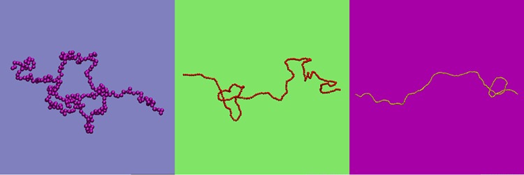
A coarse-grained computational model is used to investigate how the bending rigidity of a polymer under tension affects the formation of a trefoil knot. Thermodynamic integration techniques are applied to demonstrate that the free-energy cost of forming a knot has a minimum at nonzero bending rigidity. The position of the minimum exhibits a power-law dependence on the applied tension. For knotted polymers with nonuniform bending rigidity, the knots preferentially localize in the region with a bending rigidity that minimizes the free energy.

Type II topoisomerases are enzymes that may knot or unknot DNA by introducing a transient break in both strands of one DNA duplex and passing a second duplex through it. One of their key biological functions is to regulate the level of knotting in the genome.¹ Type II topoisomerases tend to act preferentially on certain sequences in DNA.² There is evidence that sites that are more frequently cleaved tend to be located in or next to parts of the genome called scaffold associated regions or matrix attachment regions,³⁻⁵ which are typically several hundred base pairs long³ and rich in adenine (A) and thymine (T), two of the nucleotides in DNA. Further, a specific sequence evolved in vitro, which was preferentially cleaved by a certain type II topoisomerase, was highly AT-rich.²

It is believed that AT-rich sequences are more flexible than random ones.⁵⁻⁸ For example, the work of Okonogi et al.⁷ suggests that a sequence of AT repeats is about 20% more flexible than a random sequence. An earlier study suggested that such an AT-rich sequence can have a persistence length less than half that of a GC-rich sequence.⁶ Scipioni et al.⁸ used scanning force microscopy to observe a correlation between AT-rich parts of a DNA fragment and flexibility. Further, Masilah et al.⁵ found that there is a preferentially large opening of the base pairs immediately adjacent to a preferentially cleaved site. This opening was found to be dependent on the sequence context. Opening of base pairs (bubble formation) can lead to greatly increased local flexibility.⁹ Very high flexibility at the topoisomerase II cleavage sites is probably necessary because the enzyme enforces a large bend in DNA when it binds to it.¹⁰

An intriguing question arises as to whether the correlation between the positions of cleavage sites and DNA flexibility could be important in the regulation of knotting. For example, could the variation of bending stiffness help to localize knots near cleavage sites, thus, expediting their removal? Here we make a first step toward understanding these issues by using a simple bead–spring polymer model to investigate how the free energy cost of forming a knot, ΔF_knotting, varies with polymer bending stiffness and how this influences the position of a knot within a polymer of nonuniform flexibility. In this work, we simulate only the trefoil knot, 3₁,¹¹ but our general arguments do not depend on the particular topology. Previous work¹² on how the action of type II topoisomerase may be guided by bent geometries of DNA has been performed, but variable bending stiffness was not considered.

The case of polymers under tension is biologically relevant because the action of enzymes during processes such as transcription applies forces to DNA.^12,13 In general, for polymers in a good solvent with bending stiffness, A, under tension, τ, there are three main contributions to ΔF_knotting: the reduction in entropy due the self-confinement of the polymer in the knotted region; the increase in bending energy due to the curvature enforced by the knot; and the work done against the tension in reducing the extension of the polymer, necessary to give free length for knot formation.

We consider how ΔF_knotting varies with A for fixed τ. We identify two length scales: that associated with the bending stiffness, l_A ∼ A/(k_BT), and that associated with the size of the knotted region, l_knot(A), which depends on A. When l_A ≪ l_knot(A), the main effect of increasing A will be to decrease the entropic cost of knotting and ΔF_knotting will decrease with A. Previous work on fully flexible chains (A = 0) has found knots to be weakly localized,¹⁴⁻¹⁶N_knot ∼ N^t, where N_knot is the number of monomers in the knot, N the total number in the polymer, and 0 < t < 1.¹⁴ By applying scaling arguments based on the blob picture to interpret the results of simulations of polymers under tension, Farago et al.¹⁴ estimated t = 0.4 ± 0.1. A later study used two methods, including one based on closing subsections of the polymer and calculating a knot invariant, to find t ≃ 0.75.¹⁵ The discrepancy between the two estimates may be attributed to the relatively short polymers used in the earlier work.¹⁵ Knot localization has been observed experimentally¹⁷ but is found to disappear with confinement.¹⁸ A free energy calculation for an open, linear polymer found no evidence of a metastable knot size.¹⁹

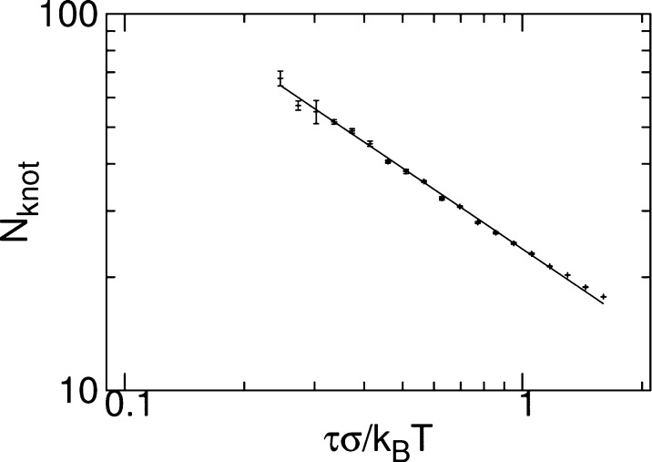
In the flexible regime, a polymer under tension will form a linear series of blobs of N_b ∼ (k_BT/τ)^1/ν monomers each, where ν ≈ 3/5.²⁰ The series of blobs cannot be knotted and so the knot resides within one blob. Treating this blob as an independent polymer, we expect l_knot to be determined by the entropic localization of the knot and the number of monomers participating to the knot to scale, accordingly, as N_knot ∼ (k_BT/τ)^t/ν. By employing the simulation techniques and knot-identification algorithm to be presented shortly, we have determined the dependence of N_knot on τ for a flexible polymer of N = 256 beads of size σ each. The results in Figure 1 indeed show a power-law dependence. By fitting to this data, we estimate that t = 0.43 ± 0.01, which is consistent with the value found by Farago et al.,¹⁴ as expected given the relatively short chains used. Concomitantly, the knot size in fully flexible chain scales as l_knot(0) ∼ N_knot^ν ∼ (k_BT/τ)^t.

Figure 1.

Variation of the number of beads forming the knot, N_knot with tension, τ for N = 256 bead flexible polymers. The solid line is a fit to the data with slope −0.71 ± 0.01. Error bars were estimated by performing three independent repeats of the simulations.

For l_A ≫ l_knot(A) the size of the knot will be dominated by the interplay of bending energy and tension and ΔF_knotting will increase with A. We therefore expect a minimum of ΔF_knotting(A) at a value of A determined by l_A ≈ l_knot(A). As the dependence of l_knot(A) on τ is not known, we replace l_knot(A) with l_knot(0) to find what the likely form of the dependence of the bending stiffness for which the free energy cost is minimal, A_min, on τ is. When the results obtained above are used, a power-law dependence is obtained:

1

Of course, the replacement of l_knot(A) with l_knot(0) in the relationship l_A ≈ l_knot(A) is an approximation that is expected to break down precisely in the region of validity of this equality. On the other hand, a power-law dependence N_knot ∼ N^t_A is a reasonable assumption also for the case A ≠ 0, thus, we anticipate a relationship of the form of eq 1 to hold also for A ≠ 0, albeit with some exponent t_A ≠ t.

For very large values of A, we expect the knot to form a single loop with the all crossings close to each other.²¹ Assuming the thickness of the polymer is small compared to the loop, we expect ΔF_knotting to be approximately given by²¹

2

For lower A, the form of ΔF_knotting may not be so easily deduced. At the crossover, this is particularly difficult because here we expect the bending length and self-confinement length to be approximately equal. For this case, a scaling form of the confinement free energy is not available.²²

We next study the consequences of these predictions with computer simulations. In what follows, we first outline the technical details of our approach, we then present results on ΔF_knotting, before investigating the positional probability distribution of knots in polymers of nonuniform flexibility. We primarily simulate single chains of N = 256 beads of size σ in a simulation box of volume V = 2.048 × 10⁵σ³ with periodic boundaries: unless otherwise stated, all results are for these parameters. The polymers are connected to themselves across the periodic boundaries in the x-direction. A constant tension is simulated by including in the potential a term proportional to the x-length of the box, L_x and allowing L_x to vary. The advantage of this approach is that there are no free ends so that, as long as chain crossings are prevented, unknotting will never occur.

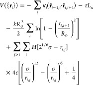
The simulation of the polymer is carried through for the following interaction potential:

3

where r_i,j = r_j – r_i, is the vector from bead i to bead j, located at position vectors r_i and r_j, respectively, whereas r̂_i,j denotes a unit vector. The first term sets the bending stiffness, which may be varied along the chain using the parameter κ_i, giving a bending stiffness of A = κ_iσ for the ith bead. The second term applies a tension, τ. The third and fourth terms are spring and excluded volume terms, respectively, H is the Heaviside step function, which truncates the Lennard-Jones potential to be purely repulsive. We choose ε = k_BT, k = 30k_BT/σ², and R₀ = 1.5σ, which prevents the chain from crossing itself and so conserves topology.

We simulate using a Monte Carlo (MC) algorithm,²³ which comprises two types of moves. To simulate a given tension, moves that attempt to change L_x, while rescaling L_y and L_z to keep V fixed and also applying a corresponding transformation to all particle coordinates, are included. Displacements of the polymer beads are made using the Hybrid MC method,²⁴ where trial states are generated using Molecular Dynamics (MD). During the MD trajectories, L_x is fixed, the tension term is not included in the Hamiltonian used to calculate the forces. Collective motions of the polymer beads are more easily captured in this way than by local, single bead moves.

To calculate ΔF_knotting for a given tension, τ, we simulate systems with all κ_i set to the same value, κ. We simulate two sets of systems, one with linear topology and one with knotted polymers. The systems within one set span a range of rigidities from κ = 0 up to the desired value. For each of those values, we calculate the average ⟨(∂V)/(∂κ)⟩. By numerically integrating ⟨(∂V)/(∂κ)⟩ from κ = 0, we obtain the relative free energy as a function of κ,²³ ΔF_α(κ) = F_α(κ) – F_α(0), where α stands for either “knot” or “linear”. To fully determine ΔF_knotting, we would need to perform an integration between unknotted and knotted states. However, because we are interested in the relative cost of knotting for different bending stiffnesses, we simply calculate ΔF_knotting(κ) – ΔF_knotting(0) = ΔF_knot(κ) – ΔF_linear(κ) instead.

To improve the efficiency of our calculation of ΔF_knotting(κ) – ΔF_knotting(0), we implemented the most computationally intensive part of our simulation algorithm on a GPU using CUDA, which allows for a high degree of parallelism but is restrictive in terms of the homogeneity of the parallel calculations.²⁵ While a standard local-move MC algorithm would be difficult to implement on a GPU,²⁵ the most time-consuming part of our algorithm is calculating the MD trajectories to produce trial states for the Hybrid MC. The MD integration may be straightforwardly performed on a GPU. We simulate all systems for a given τ and topology in parallel, performing force calculations and integration steps on the GPU. As a simple alternative to a cell list, we reduce the number of pair separations calculated by exploiting the connectivity of the polymer, which guarantees the maximum separation of two beads within a section: by comparing the center of mass positions of two sections, we can determine whether beads within them may interact. Random number generation and other MC moves were performed on the CPU. To help reduce correlation times we added parallel tempering²³ swaps between systems with different κ.

For simulations considering the positional probability distribution or size of the knot, it is necessary to determine the knotted section of the polymer. We applied a method, summarized in Figure 2, based on calculating the Alexander polynomial,¹¹A_k(x), at x = −2 for polymer subsections.²⁶ Because the polymer is extended in the x-direction by the tension, there will usually be x-positions at which only one part of the polymer crosses the y–z-plane. Regions that are bounded by such points are considered. Only one will have the correct A_k(−2). The more exact position is then found by taking subsections of this region, closing them with extensions in the ±x-direction and finding the shortest with the correct A_k(−2). The center of this section is taken as the knot position and the number of beads it contains as the knot size. This is the same method applied for the determination of N_knot for flexible chains earlier in this paper.

Figure 2.

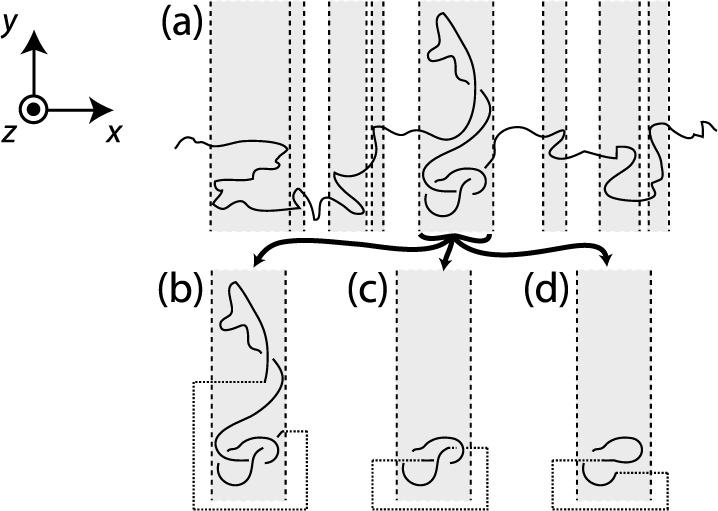
Schematic depiction of the knot-finding process. (a) The polymer is divided into sections by finding points along its contour, indicated by the dashed lines, at which there is a boundary between regions where only one strand crosses the y-z-plane and those where multiple strands do. Regions in which there are multiple crossers are identified, these are indicated by the shaded areas. They may be closed and the Alexander polynomial calculated to identify which of them contains the knot. (b–d) Subsequently, a finer determination of the knot position may be achieved by taking the knot-containing section and considering subsections of it. These are closed by extending the polymer in the x-direction, as shown by the dotted lines. The Alexander polynomial may then be calculated for each of these. The section with the correct Alexander polynomial that contains the least number of beads is taken as containing the knot. (b–d) A few examples of subsections. The subsection shown in (c) would be identified: that in (b) is contains more beads and that in (d) has the wrong polynomial.

Our procedure may occasionally result in a false identification of a knot due to extra crossings included by the closing sections. However, in previous studies the rate of such errors was found to be low and to usually involve sections larger than truly knotted ones.²⁶ We thus do not expect such pitfalls to significantly affect our results but we refer the interested reader to an in-depth consideration of such schemes.²⁷ We also found that, occasionally, no x-positions with only one crossing of the y–z-plane were found. In this case, the knot position was not identified and so these configurations were neglected. The rate of such configurations was <1% for all the results presented. As a further check, we verified that, for the knot size results, if instead of neglecting the configurations, a knot size equal to the total polymer size was added, the final averages were not changed by more than the errorbars. Simulations with knot-finding were performed with the same MC algorithm as for the free energy calculations. However, due to the computational cost of the knot-finding algorithm, which would be difficult to implement on a GPU, the calculations were performed entirely on a CPU.

We first present, in Figure 3a, results for Ψ(κ) ≡ ΔF_knotting(κ) – ΔF_knotting(0) as a function of κ for τ = 0.1, 0.4, and 0.8k_BT/σ. As expected, we observe that there is a minimum at nonzero κ, which we denote κ_min, and which decreases with increasing tension. In Figure 3b, we also plot the same data subtracting a term proportional to (8π²κστ)^1/2, the expression for ΔF_knotting at high A (eq 2 with A = σκ). The additional proportionality factor of 1.11 was determined by fitting ΔF_knotting(κ) – ΔF_knotting(0) for τ = 0.4 and 0.8k_BT/σ for κ ≥ 15k_BT. For both, the same factor was found to the accuracy that is given. The extra factor is likely necessary because our polymers do not have negligible thickness. To within errors, the curves for τ = 0.4 and 0.8k_BT/σ, with the expression subtracted, become flat for higher κ. This suggests that for these κ values we have reached the regime where ΔF_knotting is dominated by the bending and tension terms. We further observe that, at the position of the minimum of the knotting free energy cost, the quantity ΔF_knotting(κ) – ΔF_knotting(0) – 1.11(8π²κστ)^1/2 still has a relatively steep slope, confirming that the entropic contribution is important in determining the position of the minimum.

Figure 3.

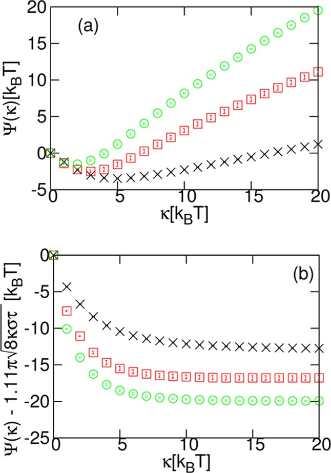
(a) Difference in free-energy, Ψ(κ) ≡ ΔF_knotting(κ) – ΔF_knotting(0), against κ for different tensions, τ: 0.1k_BT/σ (×, black); 0.4k_BT/σ (□, red); 0.8k_BT/σ (○, green). Note the minimum at κ = κ_min, which decreases for increasing τ. (b) The free-energy difference with a term proportional to the high A limit in eq 2 subtracted: Ψ(κ) – 1.11(8π²κστ)^1/2 plotted against κ for the same τ. Error bars were estimated by performing three independent repeats of the simulations.

In Figure 4, we show the dependence of κ_min on τ for N = 256. Plotting on a logarithmic scale, we see that the points for the highest five τ show a power-law relationship. Fitting to these data, we find an exponent of −0.50 ± 0.01. We, thus, obtain a power-law dependence of the optimal rigidity on the tension that we anticipated in eq 1, but with an exponent different than the t = −0.43 we found from Figure 1, as expected. For the lowest two τ we see that the curve deviates from this power-law relationship. This may be attributed to finite size effects. To verify this we repeated simulations for the three lowest τ for N = 512: the results are also plotted in Figure 4. We observe that, as expected, the results are consistent with the same power-law relationship and also follow it to lower τ.

Figure 4.

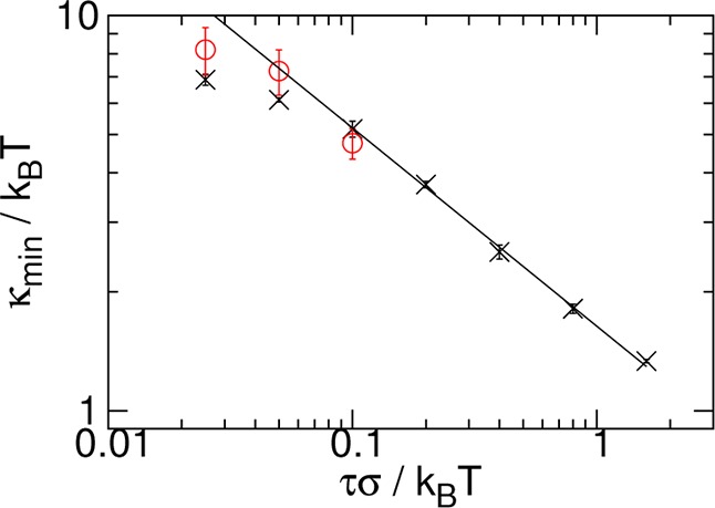
Minimum value κ_min of ΔF_knotting against the applied tension τ for N = 256 (×, black) and N = 512 (○, red). The solid line is a fit to the five data points for N = 256 with highest τ values, it has a slope of −0.50 ± 0.01. Error bars were estimated by performing three independent repeats of the simulations.

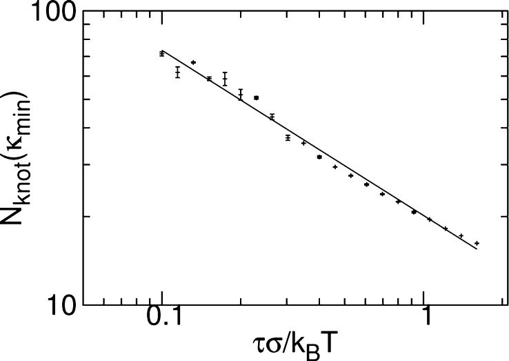
We expect κ_min to be approximately that value of bending rigidity for which the size of the knot is equal to the bending length. We consider the variation of the number of the beads in the knot at κ_min, N_knot(κ_min), with τ. We take κ_min to be given by the best fit relationship from Figure 4. We plot the results for N_knot(κ_min) in Figure 5. By fitting, we find an exponent of −0.56 ± 0.02, close to −0.50 ± 0.01: indeed, N_knot(κ_min) ∼ κ_min because the polymer is stiff at the scale of the knot.

Figure 5.

Number of bead in the knot at κ_min, N_knot(κ_min) against τ. The solid line is a fit with a slope of −0.56 ± 0.02. Error bars were estimated by performing two independent repeats of the simulations.

We have found that ΔF_knotting has a minimum at a nonzero value of the bending stiffness, namely, κ_min. We therefore expect that, if we consider a knotted polymer with nonuniform flexibility under tension, τ, the knot will be more likely to be found in a region with κ_min than in other regions. To test this, we consider a polymer of N = 512 beads at τ = 0.8k_BT/σ, split into two halves: the first 256 beads have κ_i = κ₀ ≠ κ_min. The second 256 beads have κ_i = 1.806k_BT ≈ κ_min for this τ. In Figure 6, we plot results for κ₀ = 0, 0.4353k_BT, 0.8706k_BT, and 3.842k_BT, that is, three regions with κ₀ < κ_min and one with κ₀ > κ_min. Results are binned into 8 bins of 64 beads each. In each case, we find that the probability of finding the knot in the region with κ_min is higher. In other words, the knot prefers to localize in the region where κ ≈ κ₀. Furthermore, we find that the probabilities are approximately those that would be expected from the free energy calculations. For κ₀ = 0 in Figure 6, the ratio between the average of the first four bins and that of the second four is 4.9 ± 0.5, giving an expected free energy difference of 1.6 ± 0.1k_BT. The minimum ΔF_knotting(κ) – ΔF_knotting(0) for τ = 0.8k_BT/σ in Figure 3a is −1.52 ± 0.02k_BT.

Figure 6.

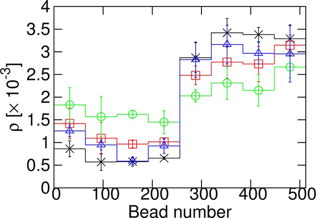
Probability density, ρ, of finding the knot at a given position along the polymer under tension, τ = 0.8k_BT/σ. For beads 256–511, κ_i = 1.806k_BT ≈ κ_min, while for beads 0–255, κ_i = 0 (×, black), κ_i = 0.4353k_BT (□, red), κ_i = 0.8706k_BT (○, green), or κ_i = 3.842k_BT (Δ, blue). Error bars were estimated by performing three independent repeats of the simulations.

To summarize, inspired by correlations between polymer flexibility and knotting seen in biology, we have investigated how the cost of forming a knot in a polymer under tension, τ, depends on the polymer’s stiffness, controlled in our model by κ. For high κ, our results agree with a simple expression including only bending and tension, while for lower κ entropy must also be taken into account. There is a nonzero minimum of the free energy difference between unknotted and knotted states at κ = κ_min. The position of the minimum is seen to depend on tension as κ_min ∼ τ^–0.5. We argue that κ_min is determined by the relative sizes of the knot and the bending length and find that the number of polymer beads in the knot at κ_min is consistent with this argument. We considered knotted polymers with two sections with different κ and found that the knot is more likely to be found in the section with κ_min.

Biological DNA is typically highly confined and in future work it would be interesting to investigate the effect of confinement on the results we have observed.^28,29 It would also be interesting to investigate how the position of cleavage sites relative to regions of different flexibility affects the steady state level of knotting,³⁰ as well as looking into how the effect of flexibility may combine with previously suggested topoisomerase II guidance mechanisms.¹² Finally, it would be intriguing to investigate how nonuniform flexibility affects the diffusional dynamics of a knot along a polymer.^31,32

The authors declare no competing financial interest.

References

- Rybenkov V.; Ullsperger C.; Vologodskii A.; Cozzarelli N. Science 1997, 277, 690–693. [DOI] [PubMed] [Google Scholar]
- Burden D.; Osheroff N. J. Biol. Chem. 1999, 274, 5227–5235. [DOI] [PubMed] [Google Scholar]
- Adachi Y.; Käs E.; Laemmli U. EMBO J. 1989, 8, 3997–4006. [DOI] [PMC free article] [PubMed] [Google Scholar]
- Razin S.; Vassetzky Y.; Hancock R. Biochem. Biophys. Res. Commun. 1991, 177, 265–270. [DOI] [PubMed] [Google Scholar]
- Masliah G.; René B.; Zargarian L.; Fermandjian S.; Mauffret O. J. Mol. Biol. 2008, 381, 692–706. [DOI] [PubMed] [Google Scholar]
- Hogan M.; LeGrange J.; Austin B. Nature 1983, 304, 752–754. [DOI] [PubMed] [Google Scholar]
- Okonogi T.; Alley S.; Reese A.; Hopkins P.; Robinson B. Biophys. J. 2002, 83, 3446–3459. [DOI] [PMC free article] [PubMed] [Google Scholar]
- Scipioni A.; Anselmi C.; Zuccheri G.; Samori B.; De Santis P. Biophys. J. 2002, 83, 2408–2418. [DOI] [PMC free article] [PubMed] [Google Scholar]
- Ramstein J.; Lavery R. Proc. Natl. Acad. Sci. U.S.A. 1988, 85, 7231–7235. [DOI] [PMC free article] [PubMed] [Google Scholar]
- Dong K.; Berger J. Nature 2007, 450, 1201–1205. [DOI] [PubMed] [Google Scholar]
- Livingston C.Knot Theory; The Mathematical Association of America: WA, 1993. [Google Scholar]
- Liu Z.; Deibler R.; Chan H.; Zechiedrich L. Nucl. Acid Res. 2009, 37, 661–671. [DOI] [PMC free article] [PubMed] [Google Scholar]
- Bustamante C.; Bryant Z.; Smith S. Nature 2003, 421, 423–426. [DOI] [PubMed] [Google Scholar]
- Farago O.; Kantor Y.; Kardar M. Europhys. Lett. 2002, 60, 53–59. [Google Scholar]
- Marcone B.; Orlandini E.; Stella A.; Zonta F. J. Phys. A: Math. Gen. 2005, 38, L15–L21. [Google Scholar]
- Mansfield M.; Douglas J. J. Chem. Phys. 2010, 133, 044903. [DOI] [PubMed] [Google Scholar]
- Ercolini E.; Valle F.; Adamcik J.; Witz G.; Metzler R.; De Los Rios P.; Roca J.; Dietler G. Phys. Rev. Lett. 2007, 98, 058102. [DOI] [PubMed] [Google Scholar]
- Tubiana L.; Orlandini E.; Micheletti C. Phys. Rev. Lett. 2011, 107, 188302. [DOI] [PubMed] [Google Scholar]
- Zheng X.; Vologodskii A. Phys. Rev. E 2010, 81, 041806. [DOI] [PMC free article] [PubMed] [Google Scholar]
- de Gennes P.Scaling Concepts in Polymer Physics; Cornell University Press: New York, 1979. [Google Scholar]
- Gallotti R.; Pierre-Louis O. Phys. Rev. E 2007, 75, 031801. [DOI] [PubMed] [Google Scholar]
- Chen J.; Sullivan D. Macromolecules 2006, 39, 7769–7773. [Google Scholar]
- Frenkel D.; Smit B.. Understanding Molecular Simulation: from Algorithms to Applications; Academic Press: London, 2002. [Google Scholar]
- Mehlig B.; Heermann D.; Forrest B. Phys. Rev. B 1992, 45, 679–685. [DOI] [PubMed] [Google Scholar]
- van Meel J.; Arnold A.; Frenkel D.; Zwart S.; Belleman R. Mol. Simul. 2008, 34, 259–266. [Google Scholar]
- Katritch V.; Olson W.; Vologodskii A.; Dubochet J.; Stasiak A. Phys. Rev. E 2000, 61, 5545–5549. [DOI] [PubMed] [Google Scholar]
- Tubiana L.; Orlandini E.; Micheletti C. Prog. Theor. Phys. Suppl. 2011, 191, 192–204. [Google Scholar]
- Dai L.; van der Maarel J.; Doyle P. ACS Macro Lett. 2012, 1, 732–736. [DOI] [PubMed] [Google Scholar]
- Matthews R.; Louis A.; Yeomans J. Mol. Phys. 2011, 109, 1289–1295. [Google Scholar]
- Vologodskii A.; Zhang W.; Rybenkov V.; Podtelezhnikov A.; Subramanian D.; Griffith J.; Cozzarelli N. Proc. Natl. Acad. Sci. U.S.A. 2001, 98, 3045–3049. [DOI] [PMC free article] [PubMed] [Google Scholar]
- Huang L.; Makarov D. J. Phys. Chem. A 2007, 111, 10338–10344. [DOI] [PubMed] [Google Scholar]
- Matthews R.; Louis A.; Yeomans J. EPL 2010, 89, 20001. [Google Scholar]