Improving detection of copy-number variation by simultaneous bias correction and read-depth segmentation

Abstract

Structural variation is an important class of genetic variation in mammals. High-throughput sequencing (HTS) technologies promise to revolutionize copy-number variation (CNV) detection but present substantial analytic challenges. Converging evidence suggests that multiple types of CNV-informative data (e.g. read-depth, read-pair, split-read) need be considered, and that sophisticated methods are needed for more accurate CNV detection. We observed that various sources of experimental biases in HTS confound read-depth estimation, and note that bias correction has not been adequately addressed by existing methods. We present a novel read-depth–based method, GENSENG, which uses a hidden Markov model and negative binomial regression framework to identify regions of discrete copy-number changes while simultaneously accounting for the effects of multiple confounders. Based on extensive calibration using multiple HTS data sets, we conclude that our method outperforms existing read-depth–based CNV detection algorithms. The concept of simultaneous bias correction and CNV detection can serve as a basis for combining read-depth with other types of information such as read-pair or split-read in a single analysis. A user-friendly and computationally efficient implementation of our method is freely available.

INTRODUCTION

Structural variation (SV), including copy-number variation (CNV), is a major form of genetic variations in mammals (1–4). CNVs have been shown to affect gene expressions in human cell lines (5) as well as in different tissues of rodents (6–8), and to play an important role in the etiology of schizophrenia (9,10), autism (11,12) and non-psychiatric diseases (13–15). In functional genomic studies, failing to account for copy-number differences can lead to errors in ribonucleic acid sequencing, chromatin immunoprecipitation sequencing, DNase hypersensitive site mapping sequencing and formaldehyde-assisted isolation of regulatory elements sequencing (16,17). Thus, accurate detection for CNVs in a single genome is important.

Microarray technologies were the main platform for initial work in CNV characterization (18,19) and remain a cost-efficient choice (20). High-throughput sequencing (HTS) technologies (21–23) promise a complete catalog of SV and could replace microarrays as a discovery platform (20,24). While microarray-based CNV detection analyzes probe hybridization intensities, HTS-based CNV detection uses conceptually distinctive approaches: read-pair, split-read and read-depth (RD) analyses, which vary in their sensitivity and specificity depending on the sizes and classes of SVs (1,20,24). Converging evidence suggests that multiple approaches should be considered together to maximize CNV detection from HTS data. For example, the 1000 Genomes Project (1000GP) used 19 algorithms to independently identify CNVs in 185 human genomes and pooled the results according to the specificity of each algorithm (1). Recent methods [SPANNER (1), CNVer (24) and Genome STRiP (25)] integrate read-pair and RD in the detection process in different ways.

The RD approach looks for higher or lower than expected sequencing coverage in a genomic region to infer gain or loss of DNA. RD has been computed in a variety of ways, including counting the number of fragments (25) or reads (26–29) mapped to a particular genomic region and calculating the sum of per-base coverage within a region (30,31). Existing CNV detection methods assume that RD follows a Poisson distribution (or a normal distribution as the large-sample approximation of the Poisson model) for a diploid genome and search for regions that diverge from this distribution. However, in practice, neither sampling nor mapping of the reads is uniform because of experimental biases. GC content can lead to certain genomic regions being over- or under-sampled (22). Repetitive DNA elements are abundant in the mammalian genomes (32); consequently, the number of reads unambiguously mapped to a region could be very different from the number of reads sequenced from the region. Additional sources of bias, which are more difficult to trace (e.g. noise arising from sequencing, sequencing errors), create further variability in RD coverage. Violation of the assumed Poisson distribution entails loss of sensitivity/specificity to detect CNVs using RD. In studies of cancer, matched pairs of tumor- and normal-tissue samples may be used to correct biases by computing RD ratios (33–36); however, matched control samples are generally not available.

Bias correction has not been adequately addressed in the literature. Some existing methods (26,28,31) adopt a two-step approach where RD is first smoothed for GC content differences using linear regression, and the GC-adjusted RD is then segmented. Other methods (25,29) account for mapping bias of a candidate region using its effective length (e.g. the number of confidently mapped bases); however, this approach does not account for the dependence between consecutive regions or additional sources of noise in the data. While various kinds of adjusted RD have been used as input data, nearly all methods (25,28–30) use the Poisson or normal-distribution assumption without subsequent evaluation the adequacy of the distributional assumption.

In this study, we first show that evaluation of the distribution assumption for RD is important, as it may not hold true. Second, we show that it is important to jointly estimate copy number and the effect of confounding factors. Third, we develop a novel statistical method to accurately model RD and detect CNVs from HTS data. We measure RD by the number of sequence fragments mapped in sliding windows tiled along the genome, and we model the fragment counts by negative binomial (NB) distributions, which allow for over-dispersion and account for the effects of confounders. Furthermore, we account for the dependence of fragment counts of adjacent windows using a hidden Markov model (HMM). Known confounding factors are treated as covariates and corrected explicitly, while unknown experimental biases are accommodated by the over-dispersion parameter of the NB distribution and by an additional noise component via a mixture model. Fourth, we calibrate our method using simulation and whole-genome sequencing data from the 1000GP, and we compare our method with CNVnator (26), the best-performing RD-based CNV detection algorithm in the literature (1). Finally, to demonstrate the utility and robustness of our method, we apply our method to both human and mouse HTS data sets.

In summary, our method outperforms existing RD-based CNV detection algorithms and distinguishes homozygous and heterozygous deletions and high-copy duplications. Our method complements the current literature, and the concept of simultaneous bias correction and CNV detection can serve as a basis for combining RD with read-pair or split-read in a single analysis. A user-friendly and computationally efficient implementation of our complete analytic protocol is freely available at https://sourceforge.net/projects/genseng/.

MATERIALS AND METHODS

Data sets included in this study

1000GP data

For method development and assessment, we used the whole-genome sequencing data from three HapMap individuals sequenced as part of the 1000GP. These include the CEU parent–offspring trio of European ancestry (NA12878, NA12891, NA12892), sequenced to 42× coverage on average using the Illumina Genome Analyzer (I and II) platform. Sequencing reads were a mixture of single end and paired end with variable lengths (36 bp, 51 bp). The complete genome sequence data were obtained in the form of ‘.bam’ alignment files from ftp://ftp.ncbi.nlm.nih.gov/1000genomes/ftp/pilot_data/data/. Reads were aligned to the human reference genome NCBI37 using BWA (37) (v.0.5.5) as described in the online documentation: ftp://ftp.ncbi.nlm.nih.gov/1000genomes/ftp/README.alignment_data.

High-confidence CNVs

To assess the sensitivity of our discovery method, we used the high-confidence CNVs established for NA12878 [Supplementary Table S6 of Mills et al.. (1)] by combining CNVs reported in earlier surveys that used high-density microarrays (2,38,39), fosmid sequencing (40) or ABI tracing mapping (41). This data set included 610 deletions [∼82% from microarray reports (2,38,39)] and 261 duplications [100% from microarray reports (2,38,39)] from the autosomes of NA12878. The second high-confidence data set used in this study was generated by Handsaker et al. (25) by accurately genotyping deletions from the 1000GP HTS data (1). The complete data set was downloaded from ftp://ftp.broadinstitute.org/pub/svtoolkit/misc/1 kg/NGPaper/ and included deletions for the three aforementioned HapMap individuals. This data set included 2301 deletions for NA12878, 2200 deletions for NA12891 and 2055 deletions for NA12892. CNV coordinates reported in both high-confidence data sets were translated from NCBI36 to NCBI37 using liftOver.

Data from other sequencing projects

To demonstrate the robustness of our method, we used HTS data from two different studies using various sequencing platforms, sequencing depths and read lengths. In the first study, we used the whole-genome sequencing data of three individuals affected with bipolar disorder from a large multiplex Spanish pedigree currently under investigation. Paired-end sequencing with 100-bp reads was performed at the University of North Carolina on the Illumina HiSeq 2000 platform. Each individual was sequenced to an average of 15× coverage. Reads were aligned to the human reference genome NCBI37 using BWA (37) (v.0.5.5) with default parameters. In the second study, we downloaded (ftp://ftp-mouse.sanger.ac.uk/current_bams/) the whole-genome sequencing data of inbred mouse strains made freely available by the Mouse Genomes Project conducted at the Sanger Institute (42). All mouse samples were sequenced on the Illumina GAII platform with a mixture of 54-, 76- and 108-bp paired reads to a coverage ranging from 17× to 43×. Reads were aligned to the mouse reference genome NCBI37 using the MAQ aligner (3,43). For this study, we analyzed the alignment files for 13 inbred strains (129S1SvlmJ, A/J, AKR/J, BALB/cJ, C3H/HeJ, CAST/EiJ, CBA/J, DBA/2J, LP/J, NOD/LtJ, NZO/HILtJ, PWK/PhJ, WSB/EiJ). We also downloaded the released SV calls for these strains from ftp://ftp-mouse.sanger.ac.uk/current_svs/. These SVs have been classified into several categories based on specific paired-end mapping patterns briefly described in Yalcin et al. (3). From this SV release, we extracted 2 categories, including deletions and copy-number gains (GAINS and TANDEMDUP), to compare with the GENSENG-predicted calls.

Reference genomes

The human reference genome NCBI37 was obtained from ftp://ftp.ncbi.nlm.nih.gov/1000genomes/ftp/technical/reference/human_g1k_v37.fasta.gz. The mouse reference genome NCBI37 was obtained from ftp://ftp-mouse.sanger.ac.uk/ref/NCBIM37_um.fa.

Input data preparation for CNV detection

Our input data are a triplet of RD signal, GC content and mappability score computed in sliding windows tiled along the genome.

RD signal

Alignment (.bam) files are parsed out using SAMtools (44) with a quality control (QC) filter to extract confidently aligned reads (see Additional file 1, Supplementary Methods). A (single-end or paired-end) sequence read represents one or two ends of a DNA fragment randomly sampled from the donor/sample genome. Using reads passing the QC filter, the RD signal is calculated as the number of sequenced DNA fragments in sliding windows, ensuring each fragment is counted only once (Supplementary Methods).

GC content

First, we calculate the proportion of G or C bases in each window from a given reference genome. Then, we apply a cubic spline smoothing and transform the GC proportion based on the fitted curve so that the transformed GC proportion and the logarithm of the RD are linearly correlated. Finally, the transformed GC proportion is median centered and is referred to as GC content hereafter.

Mappability score

As a function of both reference sequence and read length (K-mer), mappability score is calculated a priori in four steps: (i) for each base pair position in the genome, extract a K-mer from the reference genome, which consists K consecutive bases starting at this base pair position. (ii) Align the K-mers back to the reference genome using a desired aligner, e.g. BWA (37). Ideally, the aligner and the alignment parameters are chosen to match what was used for generating read alignment files from the sample genomes. (iii) Identify mappable base positions where the corresponding K-mers map back to themselves unambiguously (i.e. there is a single best hit and it is the true position of the K-mer). For example, the X0 field produced by BWA (37) relates a K-mer from a specific place in the genome to the number of best hits of that K-mer in the entire genome. If a K-mer has a X0 value of 1, the corresponding base can be identified as a mappable base. (iv) Compute mappability score as the proportion of mappable bases in a given window, which measures the uniqueness of specific regions of the reference genome.

Window consideration

The window size and the degree of overlap between them are adjusted for specific data. In this study, a window size of 500 bp with 200-bp overlap was chosen for all data sets for several reasons: first, the window size should be no less than the mean DNA fragment size of the sequencing library. Second, using a larger window size (e.g. 1 kb) or non-overlapping windows would decrease precision in defining CNV break points and miss CNVs that only partially span one window. Third, a higher degree of overlap introduces more inter-window correlation, which necessitates appropriate adjustment in modeling the RD signals.

CNV detection method

This triplet of data for each individual genome is input into an integrative HMM, which classifies each window to a copy-number state based on maximum a posteriori probability, while simultaneously accounting for sources of bias. The state changes mark the predicted break points of CNVs. Below we present a short intuitive view of our method and the elements needed in HMM characterization; full details are given in the Supplementary Methods (see Additional file 1).

Hidden states and transition probability

While microarray analysis suffers from over-saturation at high copy numbers, HTS allows RD-based methods to determine high copy numbers with improved accuracy (27). The total number of hidden states is implemented as an input parameter of GENSENG and can be freely specified by users. Theoretically, the more copy-number states specified, the more accurate the model becomes. However, a number of practical issues must be considered. For example, specifying more states means longer computing time, and for some data sets, there may not exist sufficient regions from which to estimate parameters. For the HTS data sets used in this study, we assume seven hidden states representing copy numbers of 0, 1, 2, 3, 4, 5 and 6 or more. For homozygous populations such as inbred mice, we assume four hidden states representing copy numbers of 0, 2, 4 and 6 or more. We collapse the duplications with six or more copies into one state because they are difficult to distinguish because of both experimental (reduced signal-to-noise ratio) and computational concerns (having few regions with very high RD signal).

State transitions proceed from one window to the next according to a first-order time-homogeneous Markov process. The transition probability describes the probability of having a copy-number state change between two adjacent windows. Intuitively, the copy-number state is unlikely to change for nearby windows but is more likely to change for windows that are far apart.

Emission probability

The hidden copy-number states emit probabilistic outputs at each window, i.e. the observed RD signal representing integer-valued count data. In the absence of sources of bias, sequencing coverage is uniform across the genome such that the emission probability of RD could be modeled by a Poisson distribution with equal mean and variance. In the presence of sources of bias, sequencing coverage is not uniform, and the Poisson-distribution assumption fails. To account for biases, the emission probability of RD is modeled as a mixture of uniform distribution and NB, expressed as the following:

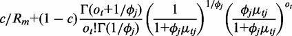where c is the mixing probability, o_t is the RD signal for window t, is the mean RD for window t given state j, is the over-dispersion parameter given state j. The uniform distribution has a density function 1/R_m to model any random fluctuation of RD, where R_m is treated as a known constant using the largest RD among all windows of the chromosome. When non-overlapping windows are used, the mean RD for each window, , is modeled by an NB regression model, where the predictors include copy-number state, GC content and mappability score. When overlapping windows are used, the observed RD is drawn from an autoregressive process; thus, a residual term is included as an additional predictor in the NB regression model assuming first-order autoregression. The additional noise in the data that cannot be explained by variability in GC content and mappability is accommodated by , the over-dispersion parameter of the NB distribution (allowing variance to be larger than mean) and the uniform distribution in the mixture model.

Tuning parameters

Given the HMM topology, the challenge lies in optimizing model parameters given the observed data, also known as HMM training. There are many parameters to be optimized. To reduce computational difficulty, we choose to specify a subset of HMM parameters based on previous knowledge and user preference, including the initial state probability, state transition probability and the mixing probability in emission probability. These tuning parameters can be influential and should be chosen carefully. The remaining emission parameters, including the coefficients and over-dispersion parameters in the NB regression model, are estimated for each data set.

Parameter estimation

The optimization problem is solved by the Baum–Welch algorithm (45), which maximizes the data likelihood for an individual chromosome in iterative steps, including initialization, expectation and maximization. In the initialization step, we rely on intuitive guesses as well as empirical values. The initial emission parameters were estimated from the 1000GP and the Mouse Genomes Project data sets where known CNVs are available. These initial emission parameters are saved for the human and mouse genomes, respectively, and are used for any new sample without previous knowledge of its CNVs. In the maximization step, we obtain maximum-likelihood estimates of emission parameters. We apply a weighted NB regression model, where the weights are posterior probabilities for each window belonging to a particular copy-number state, given the observed data of an entire chromosome. These weights represent current knowledge of the probabilistic classification of a window to copy-number state and are updated in the expectation step. While included as a predictor in the regression model, the copy number is the hidden variable to be inferred from the observed data. Intuitively, using posterior probability as regression weights, we are able to partition the observed RD across all hidden states, proportional to the likelihood. The weighted NB regression model is fitted by alternately estimating regression coefficients using iteratively reweighted least squares and estimating the over-dispersion parameter using a Newton–Raphson method. In the expectation step, we update the forward, backward and posterior probability, given the current estimates from the maximization step. The expectation and maximization steps iterate until the convergence criterion (<10⁻⁶ change in the log-likelihood) is reached.

CNV calling

Using the parameters at convergence, first we obtain the final estimates of the posterior probability for each window belonging to a particular state, given the observed data from the entire chromosome. Second, we assign the final estimate of copy number for each window using the state with the largest posterior probability. The state changes mark the predicted breakpoints of CNVs. The confidence score of a CNV region is computed as the sum of the posterior probabilities of all windows enclosed within the break points. Next, a two-step merging algorithm is carried out to refine the boundaries of the CNVs.

Prioritization of CNV calls

A CNV QC step can be applied to remove CNVs predicted with the lowest confidence. We recommend removing predicted CNVs shorter than 800 bp (i.e. removing those that appear in only one window as shown in Supplementary Table S2), or predicted CNVs with an average mappability <0.3 (i.e. removing those that cannot be confidently predicted as shown in Figure 1b). An additional prioritization approach was implemented via the RD-accessibility (RDA) statistic, which reflects the signal-to-noise ratio of a predicted CNV region after accounting for known confounders in RD. The term of RDA was first coined by Abyzov et al. (26), but for a different purpose. The RDA statistic is computed in three steps: (i) after CNV calling, identify all compatible copy-number–neutral windows the GC content and mappability scores of which are the same as those from the region of interest; (ii) calculate the average window counts from (i) as the expected RD for the region of interest; and (iii) obtain the RDA by dividing the observed RD by the expected RD for the region of interest. Using a copy number of two as normalization for copy-number–neutral autosomal regions, the theoretical signal-to-noise ratios are 0, 0.5, 1.5 and 2 for copy numbers of 0, 1, 3 and 4, respectively. Therefore, a region is considered to be RD accessible if its RDA value is <0.5 for homozygous deletions, <0.75 for heterozygous deletions and >1.25 for duplications. In general, we recommend removing CNVs predicted from regions that are not RD accessible (e.g. if its RDA values range between 0.75 and 1.25). In addition, we recommend ranking the predicted regions by their RDAs, where a higher signal-to-noise ratio reflects higher confidence that the predicted CNVs are correct; this is analogous to ranking by fold change in gene expression analysis.

Figure 1.

Relationship between read-depth and mappability in high-confidence CNVs (1). (a) The boxplot of read-depth from windows mapped to the 610 high-confidence deletions (red) and 261 high-confidence duplications (blue), suggesting a similar read-depth distribution between deletions and duplications and no power in detecting CNVs. (b) The boxplot of read-depth stratified by mappability classes, color-coded such that darker shades reflect higher mappability. The labels of the x-axis indicate the CNV class (DEL: deletions; DUP: duplications) and mappability class. For example, label (DEL: 0.2–0.3) indicates windows from the high-confidence deletions and with mappability score ranging from 0.2 to 0.3. Within each mappability class, duplications show higher mean read-depth than deletions, suggesting that correction for mappability improves the ability to detect CNVs. Furthermore, when mappability falls below 0.3, read-depth distribution becomes increasingly similar between deletions and duplications, suggesting that the ability to detect CNVs in those regions is limited. For example, for windows with mappability ranging from 0.2 to 0.3, ∼50% of windows in the duplication regions had read-depths equal to or lower than the average read-depth from compatible copy-normal regions; ∼20% of windows in the deletion regions had read-depths equal to or higher than the average read-depth from compatible copy-normal regions.

Performance assessment

While the high-confidence data set compiled by Mills et al.. (1) indicates where the true positive CNVs are for HapMap individuals, the true negatives are unknown. Therefore, we used two approaches to assess our method’s performance. First, we conducted a simulation to estimate the sensitivity and specificity to detect CNVs. Then, we analyzed the high-coverage 1000GP trio data, where we estimated the sensitivity using high-confidence CNVs and used the total number of base pairs or calls as a surrogate measure for specificity. For comparison, we applied CNVnator (26) in parallel, using its recommended parameter setup and QC filter. The methodology differences between GENSENG and CNVnator are detailed in Supplementary Table S5. The main differences are in bias correction and segmentation techniques.

Simulation

We simulated two data sets for performance assessment. The first simulation directly generated RD data (28). Using chromosome 1 from NA12878 as a template, we implanted 76 high-confidence CNVs (25 duplications and 51 deletions) (1) by assigning a copy number of four to any window that overlapped the duplications and a copy number of zero to any window that overlapped the deletions. All other windows were assigned to have a copy number of two. The covariate matrix (the assigned copy number, mappability score and GC content of each sliding window) and coefficient vector were passed to the ‘garsim’ function from R/gsarima to simulate the RD for each window. The ‘garsim’ model we applied was the NB distribution with the log link function, where the autoregressive parameter was set to 0.6, the zero correction parameter was set to ‘zq1’ and the inverse of the over-dispersion parameter was set to 0.01.

The second simulation mimicked a sequencing experiment to generate paired-end reads from a CNV containing a hypothetical chromosome. To simulate reads, we used chromosome 1 of the reference human genome as a template and modified the template sequence based on the 76 high-confidence CNVs (51 deletions and 25 duplications) (1). For any deletion, we removed the corresponding sequence of the deleted DNA, and for any duplication, we inserted an extra copy of the duplicated sequence. As a result, the implanted deletions were copy number 0 deletions, and the implanted duplications were copy number 4 duplications. Among the 76 high-confidence CNVs, eight deletions and four duplications overlap with other deletions or duplications. Thus, 64 independent CNVs were implanted (43 deletions and 21 duplications) into the chromosome 1. Second, after the CNV-containing hypothetical chromosome was created, we applied the sequencing simulator, wgsim, as implemented in SAMTools (44) to generate 36-bp paired-end short reads. For wgsim simulation, the mean value of the outer distance between the two ends was set to 200, the standard deviation was set to 20 and the sequencing error model was the empirical error model of the Illumina sequencing platform. A total of 150 million paired-end reads were generated, which gave an average sequencing coverage of 40×. Third, we used BWA (37) to map the reads to the unmodified reference human genome. The resulting alignment file was used as input to apply GENSENG and CNVnator (26). Among CNVs predicted by either approach, a true discovery was defined when a predicted CNV overlapped with at least 50% of a simulated CNV and had the same copy number.

1000GP data

We analyzed the high-coverage sequencing data for the CEU trio from the 1000GP. To facilitate the comparison between the predicted CNVs and the high-confidence CNVs, which only provide deletion and amplification calls rather than the particular copy number, we defined deletions as any GENSENG calls where the inferred copy numbers were 0 or 1, and duplications as any calls where the inferred copy numbers were >2. Sensitivity was calculated by dividing the number of total base pairs of the overlapping events (>1-bp overlap, or >50% reciprocal overlap with the high-confidence CNVs) by the total number of high-confidence CNVs.

Performance on low-coverage data

The native coverage of both our simulated data and the 1000GP high-coverage data is ∼40×. To identify the lower bound that GENSENG can handle, we applied GENSENG to data with varying sequencing coverage and compared the performance with that based on the native coverage using the same evaluation metrics. First, we repeated the simulation process as described earlier, with the targeted coverage been set as 5×, 10×, 20×, 30× and 40×. To test the consistency of our simulation, we also simulated data at 40× coverage for 10 times and observed replicable results (data not shown). Second, using the DownsampleSam.jar tool from Picard (http://picard.sourceforge.net), we down-sampled the high-coverage 1000GP data from NA12878 and achieved a series of sequencing coverage of 5×, 10×, 20×, 30× and 40×.

RESULTS

Evaluation of experimental biases in HTS

Under idealized scenarios, HTS RD is expected to follow a Poisson distribution with variance equal to the mean. However, we found that the observed variance is much greater than the mean (Supplementary Figures S1a and S2a), indicating substantial deviation from the Poisson distribution. We found that some of the non-uniformity in RD is caused by genome-wide variability in mappability and GC content. Supplementary Figures S1b and S2b show a positive correlation between mappability and RD, where low mappability scores indicate a higher proportion of repetitive sequences, resulting in lower RD; high mappability scores indicate a higher proportion of unique sequences, resulting in higher RD. Supplementary Figures S1c and S2c show a non-linear relationship between GC content and RD, where sequences with extreme GC content (low or high) tend to have lower RD. In addition to the general trends observed across various data sets, we found that the curves of RD versus GC content varied from sample to sample. For example, the peak of the mouse sample slightly shifted to the right (Supplementary Figure S2c). The fractions of mappable bases in the genomes were found to be 80–90% and increased moderately as the read-length increased (Supplementary Table S1). Lastly, we found that the non-uniformity in RD could not be explained solely by GC content or mappability. We examined the RD distribution from compatible windows that had the same GC content, had the same mappability scores and were mostly likely copy-number normal (e.g. did not overlap any high-confidence CNVs or other candidate CNVs). Then we compared the observed distribution from these compatible windows with the theoretical expectations. If GC content and mappability were the only sources of biases, the observed distribution should have closely followed a Poisson distribution. However, Supplementary Figure S3 suggests that the Poisson distribution still fails because it restricts variance to equal the mean; in contrast, the NB distribution fits the data well because its over-dispersion parameter accommodates additional sources of noise in the data.

To investigate how experimental biases impact copy-number inference, we examined the relationship between mappability and RD in high-confidence CNVs (610 deletions and 261 duplications) (1). Without accounting for mappability, duplicated and deleted regions could not be distinguished because the RD distributions were very similar (Figure 1a). However, after stratification by mappability scores, the mean RDs became significantly different between duplicated and deleted regions within a mappability class, such that these CNVs could be recovered (Figure 1b). This observation suggests that it is important to jointly estimate copy number and the effect of confounding factors. Copy-number inference made without correcting for bias may lead to systemic errors. Furthermore, as shown in Figure 1b, when mappability scores are extremely low (e.g. <0.3), too few reads can be confidently aligned to those regions, and consequently CNVs cannot be confidently predicted. This observation suggests that a CNV QC filter based on mappability score could be applied to reduce false-positive predictions.

The GENSENG method

To mitigate the effects of experimental bias and improve RD-based CNV detection, we developed a novel statistical method called GENSENG. The unique feature of GENSENG is to integrate the correction of multiple sources of bias and the inference of the copy-number states in a single analysis. Figure 2 gives an algorithmic overview of GENSENG. The tasks of input preparation were implemented in R, perl and python programming languages. The computational core of GENSENG was implemented in C++. Recommendation for the tuning parameters and initial emission parameters are provided as part of the software release. Given the input, GENSENG can report CNVs from an ∼40× human chromosome within a couple of hours.

Figure 2.

Overview of GENSENG inference framework. The required input contains two parts: the triplet data (read-depth, GC content and mappability score) and the initial parameter values. The input is passed to the GENSENG engine for parameter training based on the Baum–Welsh algorithm. To update the emission probability and the parameters for the negative binomial regression model, the weighted generalized linear model (GLM) fitting algorithm is applied iteratively, which uses the updated posterior probability of the copy-number state as the regression weights in each iteration. At the convergence of parameter training, GENSENG identifies the state with the largest posterior probability and assigns the associated copy number to the corresponding window. Finally, GENSENG outputs the coordinates of CNV segments and the confidence scores.

The methodological details of GENSENG are described in the ‘Methods’ section and in the Supplementary Methods (see Additional file 1). Briefly, the key components of GENSENG are summarized below. First, we used an HMM with seven states (0–6) for modeling of copy number. In contrast, existing methods find only two general types of copy numbers, i.e. ‘loss/deletion’ and ‘gain/duplication’. The support for the seven-state modeling strategy is evident from examples shown in Figure 3, where GENSENG correctly recovered high-confidence CNVs and identified their status as homozygous deletion, heterozygous deletion and multi-allelic duplications. Some discrepancies in the boundaries between the predicted CNVs and the high-confidence CNVs were observed, reflecting technological differences between HTS and microarrays.

Figure 3.

Example high-confidence CNVs predicted by GENSENG from the NA12878 HTS data. Each subfigure (a–e) has four panels from top to bottom, and the x-axis of each subfigure indicates genomic position in base pairs. In the first panel, the black dots on the y-axis indicate read-depth signal; red dashed lines are boundaries from GENSENG prediction; green solid lines are boundaries reported in the high-confidence CNV set (1); and grey lines are the median read-depth of the chromosome. The GC content and mappability of the region are plotted in the second and the third panels respectively. The fourth panel shows the locations of segmental duplication (purple, from the UCSC hg19 segmental duplication track) and repetitive DNAs (orange, from the UCSC hg19 repeatmask track). Shown here are a homozygous deletion (a), a heterozygous deletion (b), a simple and large duplication (c) and a complex duplication (d) that was predicted to be copy number 6+ and was right flanked by a large region with a median mappability of 0.2. Finally, (e) shows a duplication predicted to be copy number 4 from a noisy region with a median mappability of 0.58, illustrating good sensitivity for detecting duplications using simultaneous bias correction and copy-number inference.

Second, we used an NB regression model for RD and included known confounders as covariates, such that their effects on RD were removed. The emission probability of RD was made even more robust against RD outliers using a mixture model of NB and uniform distributions, such that any additional biases in the data could be modeled by the NB over-dispersion parameter and the uniform distribution. These modeling strategies permit simultaneous bias correction and CNV detection. Some of the benefits of such simultaneous analysis is illustrated in Figure 3e, which demonstrates good sensitivity for detecting duplication from a noisy region with a medium mappability score (0.58) after accounting for mappability and additional noises.

Multiple techniques were introduced in GENSENG, including correcting for GC content and mappability, modeling autoregression, fitting a mixture of NB and uniform distributions and applying QC to prioritize CNV calls (see ‘Methods’ section). To study the effects of these techniques on CNV detection and identify the best-fitting model, we examined the sensitivity and the number of CNV calls made by different partial versions of our method (Supplementary Table S2). We found that correcting for GC content alone was not sufficient; and further correcting for mappability resulted in the most substantial improvement, with gains in both sensitivity and specificity. QC including both size and RDA filters substantially improved specificity, with minimal loss in sensitivity. The best GENSENG model was selected based on these results and included all aforementioned techniques.

Performance assessment and comparison

To benchmark the performance of GENSENG, we carried out two sets of simulations. In the first simulation, we applied GENSENG to simulated RD data (sequence-fragment counts across tiled windows) for a single chromosome. For 76 simulated CNVs, we observed 88% sensitivity and 100% specificity. The remaining 12% simulated CNVs (three duplications and six deletions) did not pass CNV QC filters (RDA filter and mappability <0.3).

In the second simulation, we applied both GENSENG and CNVnator to the simulated sequence reads (instead of window read counts) for a single chromosome, and we compared the sensitivity and specificity between GENSENG and CNVnator (Table 1). Before any CNV QC filter was applied, GENSENG produced 1478 fewer false CNV calls (69% fewer false deletions and 56% fewer false duplications), demonstrating a better specificity. A total of 12 simulated CNVs (10 deletions and two duplications) were not detected by GENSENG, and they were missed because they were smaller than the minimum size of CNVs detectable by GENSENG (i.e. <800 bp), or had mappability <0.3 (i.e. unreliable regions). After the recommended CNV QC filters were applied (RDA filter for GENSENG and the default q0 filter for CNVnator), GENSENG outperforms CNVnator in both sensitivity and specificity. Specifically, for 43 simulated deletions, GENSENG had 77% sensitivity, 7% higher than CNVnator. For 21 simulated duplications, GENSENG had 90% sensitivity, 33% higher than CNVnator. The specificity for duplications was 100% for both GENSENG and CNVnator. Both methods made false deletion discoveries, but GENSENG had better specificity (1328 fewer false deletions, 12% lower false discovery rate (FDR) than CNVnator). Increasing the stringency of the CNV QC filter by removing CNVs with mappability <0.3 further improved GENSENG’S specificity (9% FDR for deletions, or 43% lower FDR than CNVnator based on the same stringent CNV QC filter), while maintaining its good sensitivity (67% for both deletions and duplications, or 15% higher sensitivity than CNVnator). This result and the result from Figure 1b suggest the usefulness of the mapability filter. In Supplementary Figure S4, we show that ranking the RDA statistic (i.e. signal-to-noise ratio after accounting for confounders) computed for each CNV is an effective approach to correctly prioritize the prediction made by GENSENG or CNVnator. Most remaining false-positive deletions in the CNVnator data set were likely influenced by multiple sources of bias, and the 52% FDR is a reasonable estimate for CNVnator based on the experimental validation conducted by the 1000GP (reported to range from 14.3 to 74.1%) (1,46). In summary, the simulation studies demonstrate that GENSENG outperforms CNVnator, suggesting that integrating bias correction from multiple sources and copy-number inference is a desired strategy for RD-based CNV detection.

Table 1.

Performance assessment based on simulated sequencing data for a chromosome

Detection method	Post-detection CNV filter	Deletions				Duplications
		Total simulated true CNVs	Total predicted CNV calls	Sensitivitya (number of true CNVs detected)	FDRb (number of false prediction)	Number of simulated true CNVs	Total predicted CNV calls	Sensitivitya (number of true CNVs detected)	FDRb (number of false prediction)
CNVnator	None	43	2171	0.94(40)	0.98(2130)	21	40	1.00(21)	0.23(9)
GENSENG	None	43	690	0.77(33)	0.95(657)	21	26	0.90(19)	0.12(4)
CNVnator	q0-filterc	43	1560	0.70(30)	0.98(1530)	21	19	0.57(12)	0(0)
CNVnator	q03+(RDA+map)d	43	48	0.53(23)	0.52(25)	21	18	0.52(11)	0(0)
GENSENG	RDAe	43	235	0.77(33)	0.86(202)	21	22	0.90(19)	0(0)
GENSENG	(RDA+map)d	43	32	0.67(29)	0.09(3)	21	16	0.67(14)	0(0)

Simulation study permits precise assessment of both sensitivity and specificity. A total of 64 true CNVs were implanted into the reference chromosome 1 (NCBI37) from which sequencing reads were simulated (see ‘Methods’ section). A true CNV is considered detected if it had >50% reciprocal overlap with the predicted CNVs.

^aSensitivity is computed as the total true CNVs detected divided by the total true CNVs. Note that a single true duplication could be overlapped by >1 predicted calls. A false prediction is any predicted CNV call that does not have >50% reciprocal overlap with any true CNVs.

^bFDR is computed as the total falsely predicted CNV calls divided by the total predicted CNV calls.

^cCNVnator filter: the default q0 filters removes any predicted calls that have >50% reads with zero-valued MAPQ (i.e. reads with multiple mapping locations).

^dOur stringent filter removes any predicted calls that have RDA values ranging between 0.5 and 1.25 or mappablility <0.3. As all simulated deletions were homozygous deletions, 0.5 was used as the lower threshold of RDA.

^eOur RDA filter removes any predicted calls that have RDA values ranging between 0.5 and 1.25.

To further evaluate GENSENG’s performance, we analyzed the 1000GP data. First, we applied both GENSENG and CNVnator to the high-coverage HTS data for NA12878 and focused on calling autosomal CNVs (Table 2). Sensitivity was estimated by comparing the predicted CNVs to the high-confidence CNVs from Mills et al.. (1) (610 deletions and 261 duplications). GENSENG gave an overall sensitivity of 56% (73% for deletions and 17% for duplications) using the 50% reciprocal overlap criterion. In contrast, CNVnator gave a lower overall sensitivity of 50% (64% for deletions and 16% for duplications) using the same criterion. Approximately 87% of the high-confidence CNVs were obtained from high-density microarrays based on changes in probe intensities (2,38,39). For these CNV regions, the evidence for changes in RD may or may not be observed from HTS data (26) (also see ‘Discussion’ section), which could be predicted by the RDA statistic. Similarly to Abyzov et al. (26), we found that ∼76% (462 of 610) high-confidence deletions were RD accessible (i.e. RDA < 0.75) from the HTS data, whereas only ∼21% high-confidence duplications (53 of 261) were RD accessible (i.e. RDA > 1.25). Given these observations, we then recomputed sensitivity by comparing the predicted CNVs with the high-confidence CNVs that are RD accessible (462 deletions and 53 duplications), which yielded an overall sensitivity of 90% for GENSENG and an overall sensitivity for 79% for CNVnator [the 79% sensitivity is similar to that reported by the authors of CNVnator (26)]. The high-confidence CNV set (1) does not provide information on the true negatives needed to assess specificity; thus, we focused on calibrating sensitivity as described above and used the volume (i.e. the total number and total base pairs) of the predicted CNVs as a surrogate measure of specificity. We found that the predicted volumes are comparable between the two methods.

Table 2.

Performance assessment based on NA12878 HTS data

Detection method	Post-detection CNV filter	Deletions			Duplications
		Total high-confidence CNVsa	Total predicted CNV calls (Mb spanned)	Sensitivityb (number of high-confidence CNVs detected)	Total high-confidence CNVsa	Total predicted CNV calls (Mbp spanned)	Sensitivityb (number of high-confidence CNVs detected)
CNVnator	q0 filterc	610	4105(142.1)	0.64(393)	261	788(9.5)	0.16(42)
GENSENG	RDAd	610	5370(48.8)	0.73(446)	261	1577(68.1)	0.17(45)
GENSENG	(RDA+map)e	610	4087(11.7)	0.7(427)	261	984(38.5)	0.15(39)

^aThe high-confidence CNV set (Mills et al. 2011) includes 610 deletions and 261 duplications, but it does not provide information on the true negatives needed to assess specificity. Thus, we focused on calibrating sensitivity and used the total number and total base pairs of the predicted CNV calls as surrogate measure of specificity. A high-confidence CNV is considered detected if it had >50% reciprocal overlap with the predicted CNVs.

^bSensitivity is computed as the total detected high-confidence CNVs divided by the total high-confidence CNVs.

^cCNVnator filter: the default q0 filters removes any predicted calls that have >50% reads with zero-valued MAPQ (i.e. reads with multiple mapping locations).

^dGENSENG filter removes any predicted calls that have RDA values ranging between 0.75 and 1.25.

^eStringent GENSENG filter removes any predicted calls that have RDA values ranging between 0.75 and 1.25 or mappablility <0.3. As deletions were either homozygous or heterozygous, 0.75 was used as the lower threshold of RDA.

Then, we applied GENSENG and CNVnator to the 1000GP HTS data from the CEU trio (NA12878, NA12891, NA12892), and we evaluated the sensitivity for detecting deletions as compared with the deletions from Handsaker et al. (25), which represent the combined CNV calls from 1000GP (1). We found that an average of 49% deletion calls from Handsaker et al. (25) intersected with GENSENG calls (Supplementary Table S3). In contrast, we found an average of∼37% intersected with CNVnator calls. The deletions reported in Handsaker et al. (25) were derived from the results from the 19 algorithms used by the 1000GP (1) and contained many deletions that are smaller than the minimum size of CNVs (<800 bp) detectable by GENSENG. For NA12878, 89% of deletions (1026 of 1148) from Handsaker et al. (25) missed by GENSENG were due to the size. Similarly, for NA12891, 51% of deletions (547 of 1072) were missed owing to the size, and for NA12892, 51% of deletions (523 of 1030) were missed owing to the size. In summary, the analyses of the 1000GP data confirm that GENSENG have better detection sensitivity than CNVnator and suggest similar or better specificity.

Finally, we demonstrate that, as expected, higher sequencing coverage improves CNV detection power, and that the lower bound of sequencing coverage that yields reasonably good performance of GENSENG is 10× (Supplementary Tables S6 and S7). GENSENG could potentially work on data sequenced to as low as 5× but with much reduced sensitivity (decreased by 33% for deletions and decreased by 10% for duplications, Supplementary Tables S6 and S7).

Application to other HTS data

As a proof of concept, we applied GENSENG to whole-genome HTS data from human and mouse samples and evaluated the validity of its prediction using an allele-sharing principle as well as additional genetic information available in our data. By allele sharing, we mean the following. From a sequencing study, genetic mutations can be readily detected with a broad spectrum of allele frequency, ranging from singleton variants that are unique to individual genomes to variants observed in multiple genomes. A variant shared among multiple genomes could arise from the inheritance of the same ancestral allele, i.e. identity by descent (IBD), such that shared variants could receive higher detection confidence. The idea of searching for shared variation to increase the power of CNV detection was previously explored by Handsaker et al. (25) in the 1000GP samples from low-coverage population-scale sequencing. In our study, we first predicted CNVs from individual genomes and then identified shared CNVs that could arise from IBD as an evaluation of GENSENG’s performance.

The three human individuals affected by bipolar disorder that we examined were cousins, and therefore, they were expected to share ∼1.5% of their genomes (1.5% IBD). If a genomic region is IBD, we expect to see a similar RD pattern for that region in each individual genome and in the pooled reads from all individuals. If the IBD region contains a true CNV, this CNV could be detected based on higher or lower than expected RD using either individual alignment files or the pooled alignment file. Known confounders such as genomic GC content and mappability could also create similarity in RD pattern across different genomes and consequently predict CNVs that are shared among them. However, because GENSENG accounts for these confounding factors while inferring copy-number states, shared CNVs that arise from such artifacts have been minimized. In summary, GENSENG identified 831 candidate CNVs that are shared among the three cousins. Shared CNVs, especially those unique to this pedigree, could indicate an enrichment of high-risk disease alleles, and these CNVs are reported elsewhere. To illustrate the utility of GENSENG, Supplementary Figure S5a shows an example of shared deletion, also included in the 1000GP SV release (1,25). This suggests that alleles segregated in the general population at an appreciable frequency (e.g. >1% in 1000GP samples) would generally be shared among multiple individuals sequenced (25). In contrast, Supplementary Figure S5b shows an example of a singleton duplication that warrants further experimental validation.

Similarly, we examined shared CNVs in the mouse genome. A genome-wide haplotype and IBD map has been established in 100 classical mouse strains using high-density single-nucleotide polymorphism(SNP) genotypes (47). Strains belonging to the same haplotype in a genomic region had >99% sequence identity and were considered IBD over that interval (47). Supplementary Figure S6 shows two examples of shared CNVs that stem from IBD. In addition, for the mouse strains, we compared the deletions and duplications predicted by GENSENG with those predicted by the Mouse Genomes Project (3,30). We found that the overall concordance rates ranged from 3 to 46% (Supplementary Table S4). A similar range of concordance was observed by the 1000GP by comparing CNV call sets generated by 19 algorithms. Furthermore, compared with the algorithms used by the Mouse Genomes Project (3,30), we found that GENSENG had higher sensitivity for detecting duplications and comparable sensitivity for deletions (Supplementary Table S4). We note that the improved sensitivity could be credited to GENSENG’s bias-correction ability, which was absent in the approaches used by the Mouse Genomes Project (3,30); this improved sensitivity warrants further experimental validation of the GENSENG-predicted duplications for the mouse strains.

DISCUSSION

We have developed a novel method, GENSENG, for detecting copy-number gain and loss from HTS data. One unique feature and a key advantage of our method is the ability to simultaneously correct for multiple sources of bias and infer CNVs from RD. The concept of simultaneous bias correction and CNV inference can serve as a basis for combining RD with read-pair or split-read in a single analysis.

The GENSENG method can be applied to whole-genome sequencing data using either single-end or paired-end reads or a mixture of the two. It does not require matched control genomes, and it does not rely on evidence from multiple individuals. The smallest CNVs that can be detected by GENSENG are 800 bp, and discrete copy numbers (0, 1, 2, 3, 4, 5 and 6+) are reported. Based on extensive benchmarking, GENSENG provides a better sensitivity–specificity profile than the previously best-performing RD-based algorithm, CNVnator (1,26), when applied to high-coverage HTS data. We have also demonstrated that our method works on both human and mouse samples with lower coverage (15×).

In the current implementation of GENSENG, the top priority has been efficient and accurate detection of simple CNVs. We used reads with unambiguous mapping to compute RD signal, which reduced the method’s sensitivity to detect complex CNVs within repetitive regions. A number of specialized algorithms have been developed to reconstruct CNVs in repeat-rich regions by considering all alignment positions (31,48–51). We used a window size of 500-bp with 200-bp overlap to compute RD, which limits the break point resolution. Currently, we are developing a refinement pipeline to locally assemble the reads at the predicted break points to define break points at base pair resolution. This feature will be available in the future release of our software.

Our likelihood-based method can be readily extended to incorporate all the sequence reads and the mapping uncertainty. In addition, we can incorporate other types of information, such as haplotype, read-pair, split-reads and allele-specific RD, that can infer allele-specific copy number. Allele-specific RD can be informative for CNV calling. For example, in one window, if we observe ∼50 reads from paternal allele and 100 reads from maternal allele, a reasonable guess is that the ratio of the number of maternal allele versus paternal allele is 1:2, which will favor copy number 3 (one paternal + two maternal), or copy number 6 (two paternal + four maternal) etc. The allele-specific RD can be incorporated as part of the emission probability, e.g. using a beta-binomial distribution similar to the setup of the B-allele frequency following the genoCN method (52).

Not all the CNVs can be detected by RD data. On examining the high-confidence CNVs, we found that ∼76% of high-confidence deletions and only ∼21% of high-confidence duplications were RD accessible from the 1000GP HTS data using 36-bp and 51-bp reads. The percentage of RD-accessible regions may increase for longer reads and when we incorporate reads that are mapped to multiple locations in the genome. In contrast, the high-confidence CNVs may be inaccurate. For example, undetected CNVs in a reference individual can lead to mistaken copy-number calls in the study samples (26,28,53). Overall, we recommend RDA ranking as an effective way for prioritizing the CNVs predicted by GENSENG because it reflects the strength of the RD signal after accounting for confounders.

Duplications are generally more challenging to detect than deletions by RD-based methods for several reasons (20,26,54). First, the RD distribution (Poisson or NB) suggests that the higher the RD signal, the larger the signal variance. As expected, RD-based methods suffer reduced sensitivity in the detection of duplications (higher variance) compared with deletions (lower variance). Second, as mentioned in the proceeding paragraph, the proportion of RD-accessible high-confidence duplications is much less than that for deletions (21% versus 76%), thus reducing the sensitivity (Table 2). Lastly, as noted by Abyzov et al. (2011) (26), abnormally high RD signal may not necessarily represent a true duplication but rather the effect of an ‘unknown reference’. QC procedures that are aimed to reduce such false-positive duplications (e.g. removing windows that are RD outlier or have any overlap with known genomic gaps) would lead to reduced sensitivity for duplications overall.

AVAILABILITY

Software and source code are available at https://sourceforge.net/projects/genseng/.

SUPPLEMENTARY DATA

Supplementary Data are available at NAR Online: Supplementary Tables 1–7, Supplementary Figures 1–6, Supplementary Methods and Supplementary References [55–60].

FUNDING

National Institutes of Health (NIH) [K01MH093517 to J.P.S.]; NARSAD Distinguished Investigator Award for general support (to P.F.S.); National Institutes of Health [R01GM074175, and R03CA167684 to W.S.]; National Science Foundation [IIS0812464 to W.W.]; National Institutes of Health [U01CA105417, U01CA134240 and MH090338 to W.W.]. Funding for open access charge: NIH.

Conflict of interest statement. None declared.

REFERENCES

- 1.Mills RE, Walter K, Stewart C, Handsaker RE, Chen K, Alkan C, Abyzov A, Yoon SC, Ye K, Cheetham RK, et al. Mapping copy number variation by population-scale genome sequencing. Nature. 2011;470:59–65. doi: 10.1038/nature09708. [DOI] [PMC free article] [PubMed] [Google Scholar]
- 2.Conrad DF, Pinto D, Redon R, Feuk L, Gokcumen O, Zhang Y, Aerts J, Andrews TD, Barnes C, Campbell P, et al. Origins and functional impact of copy number variation in the human genome. Nature. 2010;464:704–712. doi: 10.1038/nature08516. [DOI] [PMC free article] [PubMed] [Google Scholar]
- 3.Yalcin B, Wong K, Agam A, Goodson M, Keane TM, Gan X, Nellaker C, Goodstadt L, Nicod J, Bhomra A, et al. Sequence-based characterization of structural variation in the mouse genome. Nature. 2011;477:326–329. doi: 10.1038/nature10432. [DOI] [PMC free article] [PubMed] [Google Scholar]
- 4.Clop A, Vidal O, Amills M. Copy number variation in the genomes of domestic animals. Anim Genet. 2011;43:503–517. doi: 10.1111/j.1365-2052.2012.02317.x. [DOI] [PubMed] [Google Scholar]
- 5.Stranger BE, Forrest MS, Dunning M, Ingle CE, Beazley C, Thorne N, Redon R, Bird CP, de Grassi A, Lee C, et al. Relative impact of nucleotide and copy number variation on gene expression phenotypes. Science. 2007;315:848–853. doi: 10.1126/science.1136678. [DOI] [PMC free article] [PubMed] [Google Scholar]
- 6.Cahan P, Li Y, Izumi M, Graubert TA. The impact of copy number variation on local gene expression in mouse hematopoietic stem and progenitor cells. Nat. Genet. 2009;41:430–437. doi: 10.1038/ng.350. [DOI] [PMC free article] [PubMed] [Google Scholar]
- 7.Guryev V, Saar K, Adamovic T, Verheul M, van Heesch SA, Cook S, Pravenec M, Aitman T, Jacob H, Shull JD, et al. Distribution and functional impact of DNA copy number variation in the rat. Nat. Genet. 2008;40:538–545. doi: 10.1038/ng.141. [DOI] [PubMed] [Google Scholar]
- 8.Henrichsen CN, Vinckenbosch N, Zollner S, Chaignat E, Pradervand S, Schutz F, Ruedi M, Kaessmann H, Reymond A. Segmental copy number variation shapes tissue transcriptomes. Nat. Genet. 2009;41:424–429. doi: 10.1038/ng.345. [DOI] [PubMed] [Google Scholar]
- 9.Consortium IS. Rare chromosomal deletions and duplications increase risk of schizophrenia. Nature. 2008;455:237–241. doi: 10.1038/nature07239. [DOI] [PMC free article] [PubMed] [Google Scholar]
- 10.Stefansson H, Rujescu D, Cichon S, Pietilainen OP, Ingason A, Steinberg S, Fossdal R, Sigurdsson E, Sigmundsson T, Buizer-Voskamp JE, et al. Large recurrent microdeletions associated with schizophrenia. Nature. 2008;455:232–236. doi: 10.1038/nature07229. [DOI] [PMC free article] [PubMed] [Google Scholar]
- 11.Malhotra D, Sebat J. CNVs: harbingers of a rare variant revolution in psychiatric genetics. Cell. 2012;148:1223–1241. doi: 10.1016/j.cell.2012.02.039. [DOI] [PMC free article] [PubMed] [Google Scholar]
- 12.Sebat J, Lakshmi B, Malhotra D, Troge J, Lese-Martin C, Walsh T, Yamrom B, Yoon S, Krasnitz A, Kendall J, et al. Strong association of de novo copy number mutations with autism. Science. 2007;316:445–449. doi: 10.1126/science.1138659. [DOI] [PMC free article] [PubMed] [Google Scholar]
- 13.Bochukova EG, Huang N, Keogh J, Henning E, Purmann C, Blaszczyk K, Saeed S, Hamilton-Shield J, Clayton-Smith J, O'Rahilly S, et al. Large, rare chromosomal deletions associated with severe early-onset obesity. Nature. 2010;463:666–670. doi: 10.1038/nature08689. [DOI] [PMC free article] [PubMed] [Google Scholar]
- 14.Fanciulli M, Norsworthy PJ, Petretto E, Dong R, Harper L, Kamesh L, Heward JM, Gough SC, de Smith A, Blakemore AI, et al. FCGR3B copy number variation is associated with susceptibility to systemic, but not organ-specific, autoimmunity. Nat. Genet. 2007;39:721–723. doi: 10.1038/ng2046. [DOI] [PMC free article] [PubMed] [Google Scholar]
- 15.Walters RG, Jacquemont S, Valsesia A, de Smith AJ, Martinet D, Andersson J, Falchi M, Chen F, Andrieux J, Lobbens S, et al. A new highly penetrant form of obesity due to deletions on chromosome 16p11.2. Nature. 2010;463:671–675. doi: 10.1038/nature08727. [DOI] [PMC free article] [PubMed] [Google Scholar]
- 16.Laird PW. Principles and challenges of genomewide DNA methylation analysis. Nat. Rev. Genet. 2010;11:191–203. doi: 10.1038/nrg2732. [DOI] [PubMed] [Google Scholar]
- 17.Rashid NU, Giresi PG, Ibrahim JG, Sun W, Lieb JD. ZINBA integrates local covariates with DNA-seq data to identify broad and narrow regions of enrichment, even within amplified genomic regions. Genome Biol. 2011;12:R67. doi: 10.1186/gb-2011-12-7-r67. [DOI] [PMC free article] [PubMed] [Google Scholar]
- 18.Iafrate AJ, Feuk L, Rivera MN, Listewnik ML, Donahoe PK, Qi Y, Scherer SW, Lee C. Detection of large-scale variation in the human genome. Nat. Genet. 2004;36:949–951. doi: 10.1038/ng1416. [DOI] [PubMed] [Google Scholar]
- 19.Sebat J, Lakshmi B, Troge J, Alexander J, Young J, Lundin P, Maner S, Massa H, Walker M, Chi M, et al. Large-scale copy number polymorphism in the human genome. Science. 2004;305:525–528. doi: 10.1126/science.1098918. [DOI] [PubMed] [Google Scholar]
- 20.Alkan C, Coe BP, Eichler EE. Genome structural variation discovery and genotyping. Nat. Rev. Genet. 2011;12:363–376. doi: 10.1038/nrg2958. [DOI] [PMC free article] [PubMed] [Google Scholar]
- 21.Wheeler DA, Srinivasan M, Egholm M, Shen Y, Chen L, McGuire A, He W, Chen YJ, Makhijani V, Roth GT, et al. The complete genome of an individual by massively parallel DNA sequencing. Nature. 2008;452:872–876. doi: 10.1038/nature06884. [DOI] [PubMed] [Google Scholar]
- 22.Bentley DR, Balasubramanian S, Swerdlow HP, Smith GP, Milton J, Brown CG, Hall KP, Evers DJ, Barnes CL, Bignell HR, et al. Accurate whole human genome sequencing using reversible terminator chemistry. Nature. 2008;456:53–59. doi: 10.1038/nature07517. [DOI] [PMC free article] [PubMed] [Google Scholar]
- 23.McKernan KJ, Peckham HE, Costa GL, McLaughlin SF, Fu Y, Tsung EF, Clouser CR, Duncan C, Ichikawa JK, Lee CC, et al. Sequence and structural variation in a human genome uncovered by short-read, massively parallel ligation sequencing using two-base encoding. Genome Res. 2009;19:1527–1541. doi: 10.1101/gr.091868.109. [DOI] [PMC free article] [PubMed] [Google Scholar]
- 24.Medvedev P, Stanciu M, Brudno M. Computational methods for discovering structural variation with next-generation sequencing. Nat. Methods. 2009;6:S13–S20. doi: 10.1038/nmeth.1374. [DOI] [PubMed] [Google Scholar]
- 25.Handsaker RE, Korn JM, Nemesh J, McCarroll SA. Discovery and genotyping of genome structural polymorphism by sequencing on a population scale. Nat. Genet. 2011;43:269–276. doi: 10.1038/ng.768. [DOI] [PMC free article] [PubMed] [Google Scholar]
- 26.Abyzov A, Urban AE, Snyder M, Gerstein M. CNVnator: an approach to discover, genotype, and characterize typical and atypical CNVs from family and population genome sequencing. Genome Res. 2011;21:974–984. doi: 10.1101/gr.114876.110. [DOI] [PMC free article] [PubMed] [Google Scholar]
- 27.Campbell PJ, Stephens PJ, Pleasance ED, O'Meara S, Li H, Santarius T, Stebbings LA, Leroy C, Edkins S, Hardy C, et al. Identification of somatically acquired rearrangements in cancer using genome-wide massively parallel paired-end sequencing. Nat. Genet. 2008;40:722–729. doi: 10.1038/ng.128. [DOI] [PMC free article] [PubMed] [Google Scholar]
- 28.Yoon S, Xuan Z, Makarov V, Ye K, Sebat J. Sensitive and accurate detection of copy number variants using read depth of coverage. Genome Res. 2009;19:1586–1592. doi: 10.1101/gr.092981.109. [DOI] [PMC free article] [PubMed] [Google Scholar]
- 29.Medvedev P, Fiume M, Dzamba M, Smith T, Brudno M. Detecting copy number variation with mated short reads. Genome Res. 2010;20:1613–1622. doi: 10.1101/gr.106344.110. [DOI] [PMC free article] [PubMed] [Google Scholar]
- 30.Simpson JT, McIntyre RE, Adams DJ, Durbin R. Copy number variant detection in inbred strains from short read sequence data. Bioinformatics. 2009;26:565–567. doi: 10.1093/bioinformatics/btp693. [DOI] [PMC free article] [PubMed] [Google Scholar]
- 31.Sudmant PH, Kitzman JO, Antonacci F, Alkan C, Malig M, Tsalenko A, Sampas N, Bruhn L, Shendure J, Eichler EE. Diversity of human copy number variation and multicopy genes. Science. 2010;330:641–646. doi: 10.1126/science.1197005. [DOI] [PMC free article] [PubMed] [Google Scholar]
- 32.Treangen TJ, Salzberg SL. Repetitive DNA and next-generation sequencing: computational challenges and solutions. Nat. Rev. Genet. 2011;13:36–46. doi: 10.1038/nrg3117. [DOI] [PMC free article] [PubMed] [Google Scholar]
- 33.Chiang DY, Getz G, Jaffe DB, O'Kelly MJ, Zhao X, Carter SL, Russ C, Nusbaum C, Meyerson M, Lander ES. High-resolution mapping of copy-number alterations with massively parallel sequencing. Nat. Methods. 2009;6:99–103. doi: 10.1038/nmeth.1276. [DOI] [PMC free article] [PubMed] [Google Scholar]
- 34.Xi R, Hadjipanayis AG, Luquette LJ, Kim TM, Lee E, Zhang J, Johnson MD, Muzny DM, Wheeler DA, Gibbs RA, et al. Copy number variation detection in whole-genome sequencing data using the Bayesian information criterion. Proc. Natl. Acad. Sci. USA. 2011;108:E1128–E1136. doi: 10.1073/pnas.1110574108. [DOI] [PMC free article] [PubMed] [Google Scholar]
- 35.Xie C, Tammi MT. CNV-seq, a new method to detect copy number variation using high-throughput sequencing. BMC Bioinformatics. 2009;10:80. doi: 10.1186/1471-2105-10-80. [DOI] [PMC free article] [PubMed] [Google Scholar]
- 36.Ivakhno S, Royce T, Cox AJ, Evers DJ, Cheetham RK, Tavare S. CNAseg–a novel framework for identification of copy number changes in cancer from second-generation sequencing data. Bioinformatics. 2010;26:3051–3058. doi: 10.1093/bioinformatics/btq587. [DOI] [PubMed] [Google Scholar]
- 37.Li H, Durbin R. Fast and accurate short read alignment with Burrows-Wheeler transform. Bioinformatics. 2009;25:1754–1760. doi: 10.1093/bioinformatics/btp324. [DOI] [PMC free article] [PubMed] [Google Scholar]
- 38.McCarroll SA, Kuruvilla FG, Korn JM, Cawley S, Nemesh J, Wysoker A, Shapero MH, de Bakker PI, Maller JB, Kirby A, et al. Integrated detection and population-genetic analysis of SNPs and copy number variation. Nat. Genet. 2008;40:1166–1174. doi: 10.1038/ng.238. [DOI] [PubMed] [Google Scholar]
- 39.Conrad DF, Pinto D, Redon R, Feuk L, Gokcumen O, Zhang Y, Aerts J, Andrews TD, Barnes C, Campbell P, et al. Origins and functional impact of copy number variation in the human genome. Nature. 2009;464:704–712. doi: 10.1038/nature08516. [DOI] [PMC free article] [PubMed] [Google Scholar]
- 40.Kidd JM, Cooper GM, Donahue WF, Hayden HS, Sampas N, Graves T, Hansen N, Teague B, Alkan C, Antonacci F, et al. Mapping and sequencing of structural variation from eight human genomes. Nature. 2008;453:56–64. doi: 10.1038/nature06862. [DOI] [PMC free article] [PubMed] [Google Scholar]
- 41.Mills RE, Luttig CT, Larkins CE, Beauchamp A, Tsui C, Pittard WS, Devine SE. An initial map of insertion and deletion (INDEL) variation in the human genome. Genome Res. 2006;16:1182–1190. doi: 10.1101/gr.4565806. [DOI] [PMC free article] [PubMed] [Google Scholar]
- 42.Keane TM, Goodstadt L, Danecek P, White MA, Wong K, Yalcin B, Heger A, Agam A, Slater G, Goodson M, et al. Mouse genomic variation and its effect on phenotypes and gene regulation. Nature. 2011;477:289–294. doi: 10.1038/nature10413. [DOI] [PMC free article] [PubMed] [Google Scholar]
- 43.Li H, Ruan J, Durbin R. Mapping short DNA sequencing reads and calling variants using mapping quality scores. Genome Res. 2008;18:1851–1858. doi: 10.1101/gr.078212.108. [DOI] [PMC free article] [PubMed] [Google Scholar]
- 44.Li H, Handsaker B, Wysoker A, Fennell T, Ruan J, Homer N, Marth G, Abecasis G, Durbin R. The Sequence Alignment/Map format and SAMtools. Bioinformatics. 2009;25:2078–2079. doi: 10.1093/bioinformatics/btp352. [DOI] [PMC free article] [PubMed] [Google Scholar]
- 45.Baum L, Petrie T, Soules G, Weiss N. A maximization technique occurring in the statistical analysis of probabilistic functions of Markov chains. Ann. Math. Statist. 1970;41:164–172. [Google Scholar]
- 46.Consortium GP, Abecasis GR, Auton A, Brooks LD, DePristo MA, Durbin RM, Handsaker RE, Kang HM, Marth GT, McVean GA. An integrated map of genetic variation from 1092 human genomes. Nature. 2012;491:56–65. doi: 10.1038/nature11632. [DOI] [PMC free article] [PubMed] [Google Scholar]
- 47.Yang H, Wang JR, Didion JP, Buus RJ, Bell TA, Welsh CE, Bonhomme F, Yu AH, Nachman MW, Pialek J, et al. Subspecific origin and haplotype diversity in the laboratory mouse. Nat. Genet. 2011;43:648–655. doi: 10.1038/ng.847. [DOI] [PMC free article] [PubMed] [Google Scholar]
- 48.He D, Hormozdiari F, Furlotte N, Eskin E. Efficient algorithms for tandem copy number variation reconstruction in repeat-rich regions. Bioinformatics. 2011;27:1513–1520. doi: 10.1093/bioinformatics/btr169. [DOI] [PMC free article] [PubMed] [Google Scholar]
- 49.Alkan C, Kidd JM, Marques-Bonet T, Aksay G, Antonacci F, Hormozdiari F, Kitzman JO, Baker C, Malig M, Mutlu O, et al. Personalized copy number and segmental duplication maps using next-generation sequencing. Nat. Genet. 2009;41:1061–1067. doi: 10.1038/ng.437. [DOI] [PMC free article] [PubMed] [Google Scholar]
- 50.Hormozdiari F, Hajirasouliha I, Dao P, Hach F, Yorukoglu D, Alkan C, Eichler EE, Sahinalp SC. Next-generation VariationHunter: combinatorial algorithms for transposon insertion discovery. Bioinformatics. 2010;26:i350–i357. doi: 10.1093/bioinformatics/btq216. [DOI] [PMC free article] [PubMed] [Google Scholar]
- 51.Hormozdiari F, Alkan C, Eichler EE, Sahinalp SC. Combinatorial algorithms for structural variation detection in high-throughput sequenced genomes. Genome Res. 2009;19:1270–1278. doi: 10.1101/gr.088633.108. [DOI] [PMC free article] [PubMed] [Google Scholar]
- 52.Sun W, Wright FA, Tang Z, Nordgard SH, Van Loo P, Yu T, Kristensen VN, Perou CM. Integrated study of copy number states and genotype calls using high-density SNP arrays. Nucleic Acids Res. 2009;37:5365–5377. doi: 10.1093/nar/gkp493. [DOI] [PMC free article] [PubMed] [Google Scholar]
- 53.Park H, Kim JI, Ju YS, Gokcumen O, Mills RE, Kim S, Lee S, Suh D, Hong D, Kang HP, et al. Discovery of common Asian copy number variants using integrated high-resolution array CGH and massively parallel DNA sequencing. Nat. Genet. 2010;42:400–405. doi: 10.1038/ng.555. [DOI] [PMC free article] [PubMed] [Google Scholar]
- 54.Baker M. Structural variation: the genome's hidden architecture. Nat. Methods. 2012;9:133–137. doi: 10.1038/nmeth.1858. [DOI] [PubMed] [Google Scholar]
- 55.Rozowsky J, Euskirchen G, Auerbach RK, Zhang ZD, Gibson T, Bjornson R, Carriero N, Snyder M, Gerstein MB. PeakSeq enables systematic scoring of ChIP-seq experiments relative to controls. Nat. Biotechnol. 2009;27:66–75. doi: 10.1038/nbt.1518. [DOI] [PMC free article] [PubMed] [Google Scholar]
- 56.Bilmes J. A Gentle Tutorial of the EM Algorithm and its Application to Parameter Estimation for Gaussian Mixture and Hidden Markov Models. Berkeley, CA: International Computer Science Institute; 1998. [Google Scholar]
- 57.Dean C. Testing for overdispersion in Poisson and binomial regression models. J. Am. Stat. Assoc. 1992;87:451–457. [Google Scholar]
- 58.Juang BH, Rabiner LR. Mixture autoregressive hidden Markov models for speech signals. IEEE Transactions on Acoustics, Speech, and Signal Processing. 1985;Vol. ASSP-33:1404–1413. [Google Scholar]
- 59.Rabiner LR. A tutorial on hidden Markov models and selected applications in speech recognition. Proc. IEEE. 1989;77:257–286. [Google Scholar]
- 60.Venables W, Ripley B. Modern Applied Statistics with S. Verlag New York: Springer; 2002. [Google Scholar]
Associated Data
This section collects any data citations, data availability statements, or supplementary materials included in this article.