Abstract
We explore the use of diffuse optical tomography (DOT) for the recovery of 3D tubular shapes representing vascular structures in breast tissue. Using a parametric level set method (PaLS) our method incorporates the connectedness of vascular structures in breast tissue to reconstruct shape and absorption values from severely limited data sets. The approach is based on a decomposition of the unknown structure into a series of two dimensional slices. Using a simplified physical model that ignores 3D effects of the complete structure, we develop a novel inter-slice regularization strategy to obtain global regularity. We report on simulated and experimental reconstructions using realistic optical contrasts where our method provides a more accurate estimate compared to an unregularized approach and a pixel based reconstruction.
OCIS codes: (170.3010) Image reconstruction techniques, (170.6960) Tomography, (100.3190) Inverse problems, (170.3830) Mammography, (170.3880) Medical and biological imaging, (170.3660) Light propagation in tissues, (170.5280) Photon migration, (290.1990) Diffusion, (290.7050) Turbid media
1. Introduction
A wide range of applied imaging problems are concerned with the determination of a three-dimensional (3D) structure in a larger field of regard. For example, in the context of medical imaging, there is great interest of estimating vascular structures using non-ionizing modalities such as diffuse optical tomography(DOT) [1, 19]. Vessels in breast tissue are predominantly tubular structures and recovering structure and absorption values of these vessels give important information useful for breast cancer detection and determining oxygenation of the breast [1, 6]. Considering the geometry of the breast and limitations of optical modalities, reconstruction algorithms are required to handle severely limited data sets, where very few detectors are used for each source location. These challenges need to be addressed, especially considering the move of DOT to a clinical setting where data obtained from multiple patients are restricted by limited sets of source-detector pairs [1, 3, 10].
Diffuse optical tomographic image reconstruction is known to be a challenging inverse problem. The physics involved with the transport of photons through biological tissue, along with the fact that traditional measurement geometries are limited in the number of data points acquired makes the problem ill-posed, resulting in reconstructions that are sensitive to noise and un-modeled effects. Additionally, the nonlinear relationship between the parameters of interest and the measured data create significant challenges for DOT. The ill-posedness requires expensive regularization schemes or constraints on the optimization problem, while the non-linearity is traditionally addressed with linear approximations or computationally intensive non-linear forward models.
Traditionally, ill-posedness of the DOT problem has been addressed by posing image formation as the solution to an optimization problem. In this context, regularization schemes [2,4,16] are used to dampen high frequency artifacts in the recovered image. Methods such as Tikhonov and total variation regularization have been used along with L-curve methods or general cross validation to choose optimal parameters for successful regularization. Another approach is to increase the amount of data used to solve the problem. Our previous work has shown the benefit of employing hyperspectral information for accurate image recovery [12]. The non-linearity of the problem is usually dealt with by designing highly accurate numerical models, often involving finite element or finite difference methods. These approaches, although accurate, tend to impose a high computational burden, especially when the imaging moves towards the recovery of 3D structures of absorption or chromophore concentration in the breast.
In this paper we expand on our previous work of [15] where we introduced a shape-based approach based on a parametric level (PaLS) formulation for the image recovery. In that paper, under the Born approximation we assumed the absorption and reduced scattering coefficient to be known in the background, and estimated chromophore concentrations and diffusion properties of a compactly supported object of interest. A basis function expansion was used to provide a low order representation of the level set function and yielded accurate results for a highly ill-posed inverse problem. The method in [15] required no explicit regularization, and the low order nature of the model was tractable to Newton-type inversion algorithms known to converge more rapidly than gradient based schemes.
An alternative approach to shape reconstruction is presented in [5]. In this paper the authors represent a 3D object by a collection of vertically stacked unit height cylinders, which they refer to as primitives. The cross sectional density of each primitive f(r, γ) is represented as a function of a position vector r and a vector of shape parameters γ. Specifically, the function f(r, γ) is the indicator on an elliptical support where the shape of each primitive is defined by a parameter vector that holds the radius of the ellipse, the ratio of its semi-axes and the orientation angle between its semi-axes. Under this model, each object primitive is centered at a point, which corresponds to the vertical positioning of the center axis for that primitive. However, since this model was developed for generalized cylinders it is most effective when the objects are modeled as such [5].
Inspired by [5], we introduce a new, flexible approach to the modeling and estimation of 3D shapes. We define a 3D object using a set of 2D shapes, which we also refer to as primitives [5]. Our model defines each primitive as a cross-section, an infinitesimally thin area, whose structure is defined by a vector of parameters that consist of a collection of PaLS basis functions defined by their center locations, weighting factors and axis length, or dilation. The overall 3D object structure is defined by “stacking” the primitive images together, creating a parametrized approximation to a 3D object. Specifically, in 3D Cartesian coordinates (denoted by x − y − z), if z is assumed to correspond to the “vertical”, then each PaLS primitive resides in a x − z plane. This takes advantage of the tubular nature of vessels found in breast tissue [6]. The reconstruction algorithm is capable of “deactivating” any unnecessary PaLS basis functions and thereby discovering the required number of active and passive primitives to effectively reconstruct the object’s shape structure. As such, the model can effectively image multiple spatially separate anomalies, without previously defining the number of anomalous regions. Correlating adjacent slices we implement a regularization approach to augment the optimization method with a cost term associated with the assumed linear relationship between adjacent primitives. The source detector setup used for the purpose of this paper relates to an optical mammography device that we are currently designing.
The remainder of this work is organized as follows. Section 2 is devoted to a description of the forward model of the problem. Section 3 details the inverse problem and iterative technique we employ for the optimization problem. Image recovery method is discussed in Section 4 while reconstruction results using simulated and experimental data are detailed and presented in Sections 5, 6, and 7 respectively.
2. Forward problem
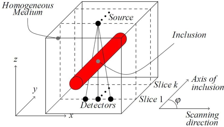
A 3D illustration of the basic sensing geometry for the tomography problem we consider is depicted in Fig. 1. In this setup, each source is scanned in tandem with detectors over the x axis, acquiring data in slices along the y axis, where detectors are restricted to the same z − x plane as the source. The medium is considered to consist of a nominal and generally homogeneous background and a collection of localized structures such as blood vessels in our application. Taking advantage of this arrangement the forward model is simplified by employing a linearization of the forward model adapted to the problem of recovering 2D slice information. Linear approximations used in DOT have been proven to produce reasonable good images in cases where the variation in optical properties within the medium is relatively small, which is the scenario often encountered in breast imaging [15, 28].
Fig. 1.
The setup of sources and detectors for simulation reconstructions. Same orientation of axes is used for experimental data. The angle φ represents the angle between the axis of the inclusion, along y in the figure, and the scanning direction, along x in the figure.
For our specific application of DOT, we implement a diffusion approximation to the radiative transport equation to model light propagation in highly scattering medium. This is given by
| (1) |
where Φ(r) is the photon fluence at position r due to light injected into the medium, v is the electromagnetic propagation velocity in the medium, is the spatially varying absorption coefficient, and S(r) = δ(r) represents a point source. Lastly D is the diffusion coefficient, given by D = v/(3μ′s) where μ′s is the reduced scattering coefficient. Here we consider uniform scattering properties that mimic those of breast tissue, hence we assume that D is constant with respect to the spatial variable r.
Under the Born (single scatter) model, we decompose the absorption, , into a constant background absorption, μa, and a spatially varying perturbation Δμa(r). This entails defining the fluence as the sum of the incident field, Φi(r), and a scattered fluence, Φs(r). To obtain a linear relationship between the measurements and the absorption concentrations, we subtract Eq. (1) from the perturbed version which leaves us with an equation for the scattered fluence
| (2) |
where and Δk2(r) = (v/D)Δμa(r). For a wide variety of unbounded and bounded geometries, the Green’s function, G(r, r′), for the operator on the left hand side of Eq. (2) can be obtained [20]. Therefore we write Eq. (2) as
| (3) |
where Δk2 = v/DΔμa in Eq. (2), rd is the location of the detector and Φi(r′, rs) denotes the incident field at position r and due to a source located at rs.
In order to approximate a 3D tubular structure using the model described in Eq. (3) we aim to reconstruct slices of a 3D medium and combine them together to estimate the underlying geometry. The physical setup is described in Fig. 1, where the source and detector are moved in tandem along the x axis, yielding K scans along the y axis. Using our forward model we define ck ∈ ℝNp as the vector of discretized μa associated with the kth slice in the rectangular region, where Np is number of pixels in each slice image, and the data collected from the corresponding slice. Using this notation we can write the forward model for the whole rectangular region in matrix vector notation as
| (4) |
where the (m, j)th element of the Kk represents the mth source-detector pair and jth pixel in the kth slice of the 3D medium. Assuming that for a given experiment Nsd source-detector pairs are used for all K slices then if Np is the number of pixels in each slice the dimensions of the whole matrix K is NsdK × NpK.
It should be noted that in our model of Eq. (4), each slice reconstruction ignores the 3D effects of the complete structure, where the primitive in each slice is assumed to be invariant along the y-axis. This has a significant impact on the accuracy of the forward model where “out-of-plane” effects on the photon migration from the overall tubular structure are not modeled by the forward model. Our method, detailed in Sections 3 and 4, of parameterizing the shape and regularization is able to recover accurate 3D structures in spite of this, even with limited data sets. Additionally this approach is easily expandable, by filling in the off-diagonal elements of K which will be considered in future developments discussed in Section 8.
3. Parametric level-set method
To counter the ill-posedness of the DOT problem we employ a Parametric Level-Set Method (PaLS). Expanding on our previous work in [15] for each slice in the 3D medium we represent the domain of the tumor as Ω ⊂ ℱ, where ℱ represents the homogeneous background which the primitive is located in, shown in Fig. 2(a).
Fig. 2.

(a) Definition of domains used for the parametric level-set methods. (b) Example basis functions placed in the imaging medium. The iteration process evolves κi and ψi towards the estimated primitive structure
We then define the support of the anomaly with a characteristic function, which describes the shape as
| (5) |
Using χ(x,y) we then represent each slice image to be reconstructed as
| (6) |
where k = 1, 2,...,K. For the purpose of reconstructing absorption concentration the unknown value in this formulation is the constant concentration values of the primitive, , and background value takes the value of the background absorption μa.
The characteristic function χ(x,y) is defined to be the τ level set of a Lipschitz continuous object function 𝒪 : ℱ → ℝ such that 𝒪 > τ in Ω(x,y), 𝒪 < τ in ℱ\Ω and 𝒪(x,y) = τ in ∂Ω. Using 𝒪(x,y), χ(x,y) is written as
| (7) |
where H is the step function where in practice we use smooth approximations of the step function and its derivative, the delta function [21].
The object function 𝒪(x,y) is represented parametrically, so instead of using a dense collection of pixel or voxel values [22], we represent it by using basis functions
| (8) |
where κi’s are the weight coefficients whereas ψi(x,y) are the functions which belong to the basis set of 𝒫 = {ψ1, ψ2,...,ψL}. Possible choices for the 𝒫 basis set include polynomial or radial basis functions, where for the purpose of this paper we use compactly supported radial basis function [18, 27]. In Eq. (8) βi defines the dilation factor of the radial basis function.
In our previous work, we reported results using the PaLS method on a fixed grid of basis functions. In that framework the goal was to strictly estimate the weight, κi, of each basis function keeping their position fixed. To ensure the adaptability of the method to different shapes we now allow each basis function to “roam” within the imaging medium. As discussed in [15] the number of basis functions, L, used in a fixed grid framework directly affected the results, and sometimes resulted in reconstruction errors. By removing the fixed grid, and instead estimating the centers of the basis functions allows for greater accuracy and adaptability for the method. We represent the center point of the ith basis function as ri = (xi, yi).
In this new formulation, all the parameters of the model are gathered in one vector where K represents the number of slices, where L basis functions reside giving κk = [κ1,..., κL]T, βk = [β1,..., βL]T and rk = [ri,..., rL]T. Now our forward model in Eq. (4) can be expressed as
| (9) |
This parameterization of the forward model contains far fewer unknowns than a pixel based method and allows for high adaptability with the movable basis functions. As an example, a single image with 4544 pixels is reconstructed using 21 basis functions, requiring only 85 unknowns.
We denote the total number of 2D PaLS primitives by K, and the plane in which the kth primitive resides as y = yk, where k = 1,...,K and the number of basis functions by L in each plane where l = 1,...,L. For simplicity, we assume that the primitives are equally spaced, though this assumption can be easily relaxed. Thus far, our model only defines the object at K points on the y-axis, where in essence the primitives may be interpreted as cross section of the overall 3D object. The object description at all other points on the y axis is recovered independently, and then combined to represent the 3D structure.
4. Image reconstruction
The image reconstruction method, recovering c from Φs, is formed as a regularized optimization problem of the form
| (10) |
where W represents the structure of the noise corrupting the data. The first term in Eq. (10) requires that the estimated value of c is consistent with the observed measurement of Φs. The second term of Eq. (10) is a regularization term that correlates the parameter vector between slices. Considering the prior information of tubular structure anatomy of breast tissues, it encourages correlating reconstructions between slices in the cost functional. Therefore the second term Eq. (10) ensures that a reconstruction between slices will result in connected structures, which provides better approximation of the structure than a unregularized function. We structure L to penalize the difference between similar parameters on adjacent primitives. That is to say, we impose a penalty for the difference between centers, ri and ri+1 for i = 1,...,K − 1, the value of absorption, and weight κi so that L is given by.
| (11) |
Where I is a diagonal matrix where number of diagonal elements are the same as number of elements in θk, and A ⊗ B is the Kronecker product [13] of A and B and Ld is written as
| (12) |
In order to demonstrate the effectiveness of our regularization method, we evaluate a tomographic reconstruction over a range of values for the regularization parameter α. As α is varied the algorithm trades off the cost associated with the regularization penalty against the cost associated with the data. To select the optimal regularization parameter we employ the commonly used L-curve method, detailed in Section 7 [7].
The W matrix reflects the structure of the noise corrupting the data [9]. We employ a Gaussian noise in which independent, zero mean Gaussian noise is assumed to corrupt each datum. Letting denote the variance of the noise corrupting the mth elements of Φ, W is constructed as a diagonal matrix with 1/σm the mth element along the diagonal. For the experimental and simulated data the variance is calculated from
| (13) |
where Ω(m) corresponds to the photon count for each source-detector pair. The SNR for each element of Φ is then calculated from
| (14) |
In experimental data is the standard deviation of the Poisson noise distribution. The minimization of the cost function is then achieved by the Levenberg-Marquardt algorithm. For that purpose an error vector, is introduced where each term relates to the corresponding term in Eq. (10) given as
| (15) |
| (16) |
In order to employ the Levenberg-Marquardt algorithm, the calculation of the Jacobian matrix J is required. The Jacobian contains derivatives of ε with respect to each element in the parameter vector θ
| (17) |
The solution is then obtained by updating θ at each iteration as θn+1 = θn + h where h is the solution to the following linear system
| (18) |
where I is the identity matrix, ρ is the damping parameter affecting the size and direction of h and found via and appropriate line search algorithm [23]. The stopping criteria used when iterating Eq. (18) is the discrepancy principle [24], in that the iterations are stopped when the norm of the residual has reached the noise level within a certain tolerance.
5. Simulation analysis
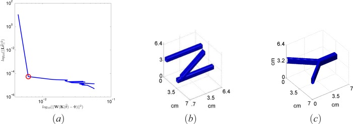
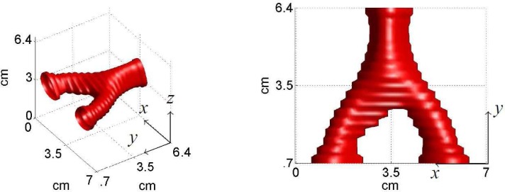
Simulations are done to demonstrate the benefit of combining simple 2D reconstructions of more than one slice to approximate 3D structure. In this paper, simulated data are generated using a standard finite difference discretization scheme for a rectangular box with dimensions 7 cm × 7 cm × 6.3 cm discretized into a 71 × 71 × 64 grid. Two simulated phantoms are created, phantom 1 with three cylinders placed close to the center, and phantom 2 with a single branching structure. phantom 2 is used for preliminary testing of our method to recover branching cylinders, which are commonly found in vascular structures. Boundary conditions on the source and detector planes are Robin type conditions, and Dirichlet conditions are applied the sides of the box in the z − x and z − y planes. The true geometries of phantoms 1 and 2 are shown in Fig. 3(b) and (c), respectively. Each cylinder in the medium has Δμa = 0.04 cm−1 where the background has μa = 0.02, giving absorption contrast of 2:1, comparable to what is found in a clinical setting [25]. Diffusion coefficient is assumed to be constant throughout the medium and inclusion at μ′s = 10.1 cm−1 at 690 nm [26]. For the simulated data the Green’s functions in (2) are obtained by computing the finite difference solution for each light source position and detector for the homogeneous background.
Fig. 3.
(a) Example L-curve used to select optimal α for the reconstruction in Fig. 7. (b) Ground truth used to generate phantom 1, with multiple overlaying cylinders. (c) Ground truth image used to generate phantom 2, with a single branching structure.
The alignment of sources and detectors is the same as for the experimental setup shown in Fig. 1. Two different cases are considered, to demonstrate the effect of limited data for our method. In case 1 we use 2 detectors per source position and 26 source locations along each slice for a total of only 52 measurements per slice. In case 2 we implement 10 detectors for each source position, giving 260 source detector pairs for each slice. These two cases demonstrate the effectiveness of our method even when working with severely limited data such as in case 1. We demonstrate reconstruction results for phantom 2 only using 10 detectors.
In order to obtain a quantitative measure of comparison between the actual and estimated shapes and absorption values, we employ two performance metrics, as follows. Designated by Sest the 0 − 1 characteristic matrix corresponding to the estimated shape, and Sact the 0 − 1 characteristic matrix corresponding to the actual object. Let Nv denote the number of overall voxels in the region of interest with i denoting the ith element of Sest and Sact. Symmetric Difference, dsd, is the fraction of entries in Sest where the corresponding entries in Sact are not equal. Mathematically, this is expressed as
| (19) |
where 1{·} is the indicator function. Another metric to judge shape estimation the Dice coefficient, ddi, measures the similarity between Sest and Sact judge how well the concentrations are located by computing
| (20) |
where a perfectly reconstructed image gives ddi = 1 and failure gives ddi=0. Finally the Mean Square Error, MSE, measures how well the reconstructed structure ĉ recovers the true absorption values and shape c, computed by
| (21) |
The symmetric distance is an important measure of the quality of reconstruction because it measures the overall quality of shape reconstruction, by penalizing errors in detecting object voxels as background and similarly background voxels as object voxels. Symmetric difference assigns an equal penalty to an erroneous voxel, irrespective of whether it is detected as background or object. An important limitation of the symmetric difference measure is that it does not reflect well on how close the estimated absorption concentration value in the reconstructed image is to the true value. The mean square error fills this gap by providing a measure on the quantitative accuracy for each slices that measures both how well the shape and value of the Δμa is recovered.
As discussed in Section 1 our method constrains the image formation problem and reduces the number of unknowns when compared to a traditional pixel-based approach. To demonstrate the effectiveness of our approach we perform pixel-based reconstructions for the simulation cases presented in Section 7. We employ a pixel-based optimization method using Levenberg-Marquardt algorithm where we modify Eq. (10) so that the regularization term takes the form of traditional Tikhonov regularization, where L = I. Tikhonov regularization is widely used for image reconstruction for multiple imaging modalities and provides a suitable comparison for our method [4, 16, 29].
6. Experimental analysis
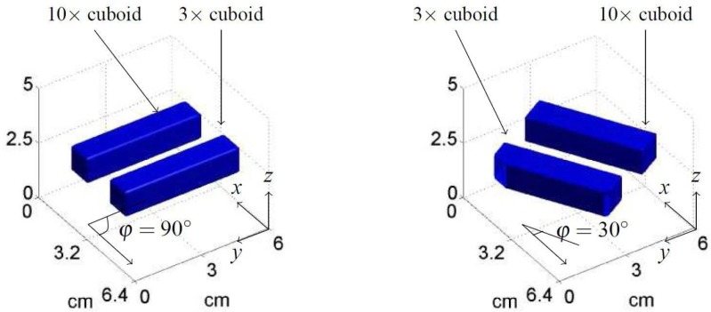
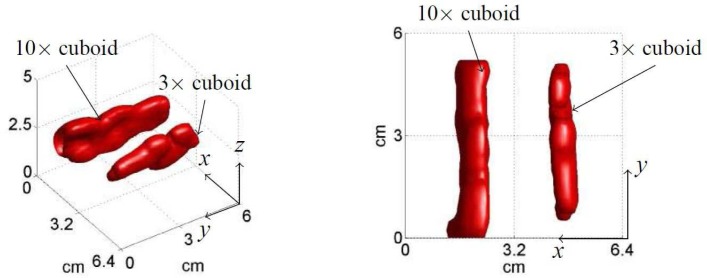
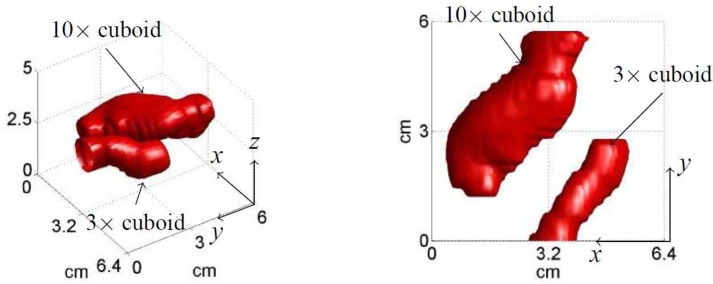
A silicon phantom was constructed in the shape of a 5 cm thick homogeneous slab, with μa = 0.16 cm−1 and μ′s = 10.1 cm−1 at 690 nm. Embedded in the slab are two absorbing cuboids, each with a height and width of 1 cm and length of 4.5 cm, separated by 1.6 cm. The geometry of the inclusions embedded in the phantom is shown in Fig. 4. In this experimental setup we utilize analytical Green’s functions for the forward model in Eq. (4). The cuboid inclusions have the same μ′s as the slab and their μa is ten and three times higher than the background, respectively. The 10× absorption results in a highly absorbing rod, where we define Δμa = 1.28 cm−1 for ground truth comparison, where the 3× cuboid has Δμa = 0.33 cm−1. The 10× absorbing rod has high absorption, mimicking the strong absorption of blood where the 3× rod is close to realistic values for breast cancer. This experimental setup allows us to test our algorithm to recover realistic tubular structures accurately even when highly absorbing areas, exceeding the Born approximation limit, are present in the medium [8, 25].
Fig. 4.
Calculated ground truth images for phantom angled at φ = 90° and φ = 30° relative to scanning direction along the x-axis.
Two different measurements are performed to test the robustness of the approach when inclusions are angled with respect to the scanning direction. The angle φ is defined as the angle between the direction of the cuboids and the scanning direction, as shown in Fig. 1. The first set is obtained where the inclusions are exactly perpendicular to the scanning direction, φ = 90°, and a second set where φ = 30°. These two setups are demonstrated in Fig. 4. The instrument performs a two dimensional planar scan, with an illumination and detection fiber operating in transmission geometry. For three different detector positions at x = {±1, 0} cm a light source is placed on the opposite side of the phantom using a 4 mm diameter fiber. For each scan 32 light sources are considered with 0.2 increments resulting in 96 source-detector pairs for each slice, where slices are spaced 0.2 cm along the y-axis. Using a Xenon arc lamp light source emitting a power of 13 mW, optical data is then found by spatially sampling 25 points/cm2 at wavelengths from 650–900 nm. The light is collected by an optical fiber that delivers light to a spectrograph (Model No. SP-150, Acton Research Corp., Acton, MA) with a 2 mm wide slit entrance. The wavelengths are resolved by a cooled CCD Camera (Model No. DU420A-BR-DD, Andor Technology, South Windsor, CT) giving a spectral sampling rate of 0.5 nm−1. Reconstructions are performed at a wavelength of 690 nm. Considering the geometry of the phantom we use the Green’s functions for slab geometry [14], computed by
| (22) |
where , , and represent the negative and positive sources used for calculation, respectively.
7. Results
7.1. Simulations
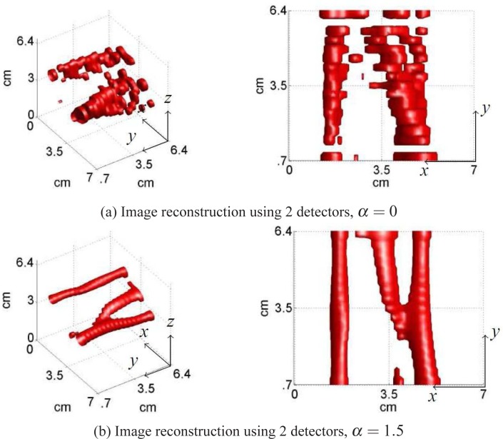
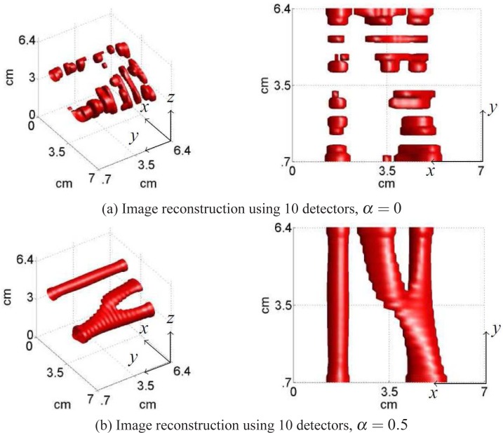
Reconstruction results from simulated phantom 1 are presented in Figs. 6, 7 using 2 detectors and 10 detectors for each source location, respectively, and Fig. 9 shows reconstruction results for phantom 2 using 10 detectors. Examining the reconstructions visually and with the error metrics presented in Table 1 it is evident that the impact of correlation regularization is very important. Especially notable is where unregularized reconstruction, shown in Figs. 6(a) and 7(a) recovers a structure with gaps, due to the fact that the connected nature of the tubular structure is not being enforced. Additionally, as is made evident by the shape metrics ddi and dsd the middle rod is recovered as a separate structure when the regularization is present. Reconstruction results for the branching structure of phantom 2 is shown in Fig. 9 with corresponding error metrics are shown in Table 1.
Fig. 6.
Reconstruction results from simulated data, phantom 1, with realistic optical contrast, using 2 detectors for each source location. Recovered absorption values are Δμa = 0.015 and Δμa = 0.019, for Fig. (a) and (b), respectively.
Fig. 7.
Reconstruction results from simulated data, phantom 1, with realistic optical contrast, using 10 detectors for each source location. Recovered absorption values are Δμa = 0.021 and Δμa = 0.026, for Fig. (a) and (b), respectively.
Fig. 9.
Reconstruction results from simulated data, phantom 2, using 10 detectors for each source location. Recovered absorption value is Δμa = 0.020.
Table 1.
Error metrics used to judge image reconstructions for simulated reconstructions.
| Fig. | # detectors | α | ddi | dsd [%] | MSE |
|---|---|---|---|---|---|
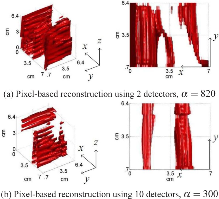
| 5(a) | 2(pixel-based) | 820 | 0.07 | 76 | 9.50 |
| 5(b) | 10(pixel-based) | 300 | 0.08 | 74 | 8.30 |
| 6(a) | 2 | 0 | 0.43 | 11 | 1.20 |
| 6(b) | 2 | 1.5 | 0.83 | 10 | 0.90 |
| 7(a) | 10 | 0 | 0.57 | 12 | 1.10 |
| 7(b) | 10 | 0.5 | 0.82 | 9 | 0.89 |
| 9 | 10 | 1.2 | 0.78 | 10 | 0.92 |
Pixel-based reconstruction using traditional Tikhonov regularization is shown in Fig. 5 for both the 2 detector and 10 detector setup. It is evident both by visual inspection and error metrics shown in Table 1 that the constrained model in PaLS and regularizing between slices results in a far more accurate estimation of the structure. It should be noted that pixel based reconstructions for DOT can be very accurate, however as mentioned above the work in this paper presents results using a severely limited dataset. Pixel-based methods traditionally require significant number of data points, resulting in the errors in the reconstruction shown here.
Fig. 5.
Reconstruction results for a simulated data, phantom 1, with realistic optical contrast. Recovered absorption values are Δμa = 0.018 and Δμa = 0.022, for Fig. (a) and (b), respectively.
As mentioned in Section 4, to estimate a near optimal regularization parameter α we implement the L-curve method. In this method, we generate a plot of log(‖Lθ‖2) against log(‖W(K(θ) − Φ)‖2) as α is varied. Fig. 6(a) depicts the reconstructed object when α = 0, where no regularization is being applied. From visual observation as well as examining error metrics defined in Section 5, it is clear that some degree of regularization is beneficial. The L-curve plot for the reconstruction of the simulated phantom is shown in Fig. 3(a). Note the encircled point on the curve denotes the “best” reconstruction given the data. The parameter α was obtained in a similar fashion in all our experiments. However, here in order to save space, we have only demonstrated our results for a single case.
Representative slice image from the 10 detector reconstruction is shown in Fig. 8. Along with the MSE it allows for visually judging the methods ability to recover the values of Δμa. As expected using the Born Approximation, the absorption values are underestimated, but these results are encouraging, considering the limited data sets being employed, and how each slice reconstruction is not modeled to incorporate effects from the total 3D structure.
Fig. 8.
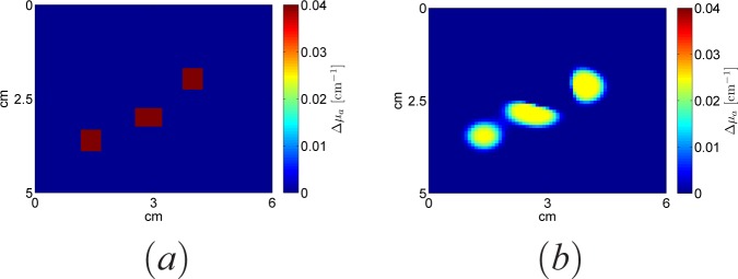
(a) Slice reconstruction, shown on the bottom, located at y = 5 cm in Fig. 7(b), compared to (b) ground truth, shown on top, demonstrating absorption perturbation, Δμa.
These results are especially encouraging considering the method is able to estimate the structure even with a severely limited data set, shown in Fig. 6, where only 2 detectors are used for each 26 source locations, and only a single wavelength is used. This demonstrates the ability of the slice based PaLS method to accurately recover 3D tubular structures even with linear approximations and limited data sets. Additionally the PaLS method is able to recover branching structures without decision making or prior information, by taking advantage of correlation in between slices.
7.2. Experimental validation
Reconstruction results for relative absorption reconstructions are shown in Figs. 10 and 11 for inclusions angled at 90° and 30°, respectively. As demonstrated in simulations, including correlation between adjacent slices greatly improves accuracy and allows for recovery of the underlying structure. Examining the images along with the error metrics, ddi, dsd and MSE shown in Table 2 it is clear that this method allows for recovery of tubular structures in a realistic breast phantom. It is notable that the 10× absorbing inclusion is recovered as a larger structure, whereas the 3× cuboid is recovered close to its true shape with more accurate absorption value. This is demonstrated in an example slice image for the φ = 90° case in Fig. 12. This is expected due to the aforementioned limitations of the Born Approximation [17] but it is interesting to see, that the higher absorbing structure does not dominate the optimization and our method correctly locates and recovers the 3× cuboid. Although the recovered absorption contrast does not improve greatly for the φ = 30° case, although shape is recovered much better when regularization is introduced. For the 30° case improvements in both absorption values and shape are evident and examining Fig. 11 shows clearly that we are able to recover structures even though they are angled close to the scanning direction. The correlation term in Eq. (10) is shown to be as important for experimental reconstructions as in simulations, both in error metrics in Table 2 and visually, in Fig. 11(a). For both experimental sets, the primitive 3D PaLS method resolves the location and the shape of the inclusion more accurately, which is verified by all metrics. It should be noted in Table 2 that ddi is computed strictly for regions where the inclusions are present. This is due to the Dice coefficient not being a useful metric to judge reconstructions when the ground truth is an empty set image.
Fig. 10.
Reconstruction results using experimental data and 3 detectors. Inclusions are angled 90° relative to scanning direction, α = 12. Recovered absorption contrast is 2.75, slice image shown in Fig. 12.
Fig. 11.
Reconstruction results using experimental data and 3 detectors. Inclusions are angled 30° relative to scanning direction, α = 80. Recovered absorption contrast is 2.30.
Table 2.
Error metrics used to judge image reconstructions for experimental reconstructions.
| Fig. | φ | α | ddi | dsd [%] | MSE |
|---|---|---|---|---|---|
| 10(a) | 90° | 0 | 0.23 | 8.6 | 0.99 |
| 10(b) | 90° | 12 | 0.55 | 6 | 0.97 |
| 11(a) | 30° | 0 | 0.31 | 13.6 | 1.10 |
| 11(b) | 30° | 80 | 0.65 | 10 | 0.98 |
Fig. 12.
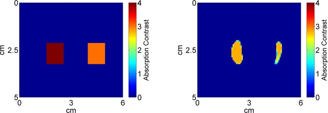
Slice reconstruction, shown on the right, located at y = 3 cm in Fig. 10, compared to ground truth, shown on the left, demonstrating absorption contrast.
8. Conclusion
Using both simulations and experimental measurements we have shown that 3D tubular structures can be recovered by implementing a parametric primitive PaLS method by taking advantage of correlation of adjacent slices. Using an augmented cost function and optimizing regularization results in better performance compared to pixel based and unregularized shape based approach measured in terms of MSE and spatial localization as measured using the Dice coefficient and Symmetric difference. This shows that even with implementing linear approximation and using severely limited data sets, the underlying structures can be recovered with accuracy.
Based on the results reported on in this paper we want to improve on this method by testing it with more cases of silicon phantoms, as well as complicated multiple branching structures, exploring how the effect of low absorption contrasts changes the recovery of structures. Furthermore the plan is to develop system that combines optical mammography measurements with depth information of vascular structures and the method presented here to serve as initial guesses for a full 3D non-linear reconstruction. Providing an accurate initial guess for a 3D non-linear reconstruction would not only improve accuracy but significantly speed up computation time commonly found in those types of reconstructions. Additionally our method is readily expandable to a model where interpolation functions can be applied to the primitives between slices, where nth order hold functions, sinc functions, or spines could be used to interpolate the primitives to represent the 3D structures. Future work will also expand the algorithm to recover images of multiple chromophore concentrations, as well as scattering amplitude. This can be achieved with minor changes to our method, and has been previously demonstrated with the PaLS method [15].
As discussed in Section 2 our model assumes that for each slice the primitive is invariant along the y-axis. This of course significantly affects the mismatch between the model and the true scenario, but our method demonstrated that correlating the slice images and parameterizing the reconstruction allows for accurate recovery of the vessel like structures. Future efforts will examine the effect of computing the off diagonal elements of Eq. (4) where it would be see how results would change if a certain segment along the y-axis would be modeled in 3D. This would physically represent stacking 3D slices with a certain thickness to recover a larger 3D structure and examining reconstruction accuracy versus computational intensity is a natural progression of our research.
Acknowledgments
We thank Geethika Weliwitigoda for help with initial testing of the algorithm and experimental data. This research is supported by the National Institutes of Health grant R01 CA154774.
References and links
- 1.Yang Y., Sassaroli A., Chen D. K., Homer M. J., Graham R. A., Fantini S., “Near-infrared, broad-band spectral imaging of the human breast for quantitative oximetry: applications to healthy and cancerous breasts,” J. Innov. Opt. Health Sci. 3, 267–277 (2010). 10.1142/S179354581000112X [DOI] [Google Scholar]
- 2.Li A., Zhang Q., Culver J. P., Miller E. L., Boas D. A., “Reconstructing chromosphere concentration images directly by continuous diffuse optical tomography,” Opt. Lett. 29, 256–258 (2004). 10.1364/OL.29.000256 [DOI] [PubMed] [Google Scholar]
- 3.van de Ven S., Wiethoff A., Nielsen T., Brendel B., van der Voort M., Nachabe R., Van der Mark M., Van Beek M., Bakker L., Fels L., Elias S., Luijten P., Mali W., “A novel fluorescent imaging agent for diffuse optical tomography of the breast: first clinical experience in patients,” Mol. Imaging Biol. 12, 343–348, 2010 10.1007/s11307-009-0269-1 [DOI] [PMC free article] [PubMed] [Google Scholar]
- 4.Yalavarthy P. K., Pogue B. W., Dehghani H., Carpenter C. M., Jiang S., Paulsen K. D., “Structural information within regularization matrices improves near infrared diffuse optical tomography,” Opt. Express 15, 8043–8058 (2007). 10.1364/OE.15.008043 [DOI] [PubMed] [Google Scholar]
- 5.Bresler Y., Fessler J. A., Macovski A., “A bayesian approach to reconstruction from incomplete projections of a multiple object 3D domain,” IEEE Trans. Pattern Anal. Mach. Intell. 2, 840–858 (1989). 10.1109/34.31446 [DOI] [Google Scholar]
- 6.Jesinger R. A., Lattin G. E., Ballard E. A., Zelasko S. M., Glassman L. M., “Vascular abnormalities of the breast: arterial and venous disorders, vascular masses, and mimic lesions with radiologic-pathologic correlation,” Radiographics 31, E117–E136 (2011). 10.1148/rg.317115503 [DOI] [PubMed] [Google Scholar]
- 7.Belge M., Kilmer M. E., Miller E. L., “Efficient determination of multiple regularization parameters in a generalized l-curve framework,” Inverse Probl. 18, 1161–1183 (2002). 10.1088/0266-5611/18/4/314 [DOI] [Google Scholar]
- 8.Fantini S., Sassaroli A., “Near-infrared optical mammography for breast cancer detection with intrinsic contrast,” Ann. Biomed. Eng. 40, 398–407(2011). 10.1007/s10439-011-0404-4 [DOI] [PMC free article] [PubMed] [Google Scholar]
- 9.Gaudette R. J., Brooks D. H., DiMarzio C. A., Kilmer M. E., Miller E. L., Gaudette T., Boas D. A., “A comparison study of linear reconstruction techinques for diffuse optical tomographic imaging of absorption coefficient,” Phys. Med. Biol. 45, 1051–1069 (2000). 10.1088/0031-9155/45/4/318 [DOI] [PubMed] [Google Scholar]
- 10.Dehghani H., Pogue B. W., Poplack S. P., Paulsen K. D., “Multiwavelength three-dimensional near-infrared tomography of the breast: Initial simulation, phantom, and clinical results,” Appl. Opt. 42, 135–145 (2004). 10.1364/AO.42.000135 [DOI] [PubMed] [Google Scholar]
- 11.Culver J. P., Ntziachristos V., Holboke M. J., Yodh A. G., “Optimization of optode arrangements for diffuse optical tomography: A singular-value analysis,” Opt. Lett. 26, 701–703 (2001). 10.1364/OL.26.000701 [DOI] [PubMed] [Google Scholar]
- 12.Larusson F., Fantini S., Miller E. L., “Hyperspectral image reconstruction for diffuse optical tomography,” Biomed. Opt. Express 2, 947–965 (2011). 10.1364/BOE.2.000946 [DOI] [PMC free article] [PubMed] [Google Scholar]
- 13.Laub A. J., Matrix Analysis for Scientists and Engineers, 1st ed. (Society for Industrial and Applied Mathematics, 2004), [Google Scholar]
- 14.Martelli F., Del Bianco S., Ismaelli A., Zaccanti G., Light Propagation through Biological Tissue and Other Diffusive Media, 1st ed. (SPIE, 2009). [Google Scholar]
- 15.Larusson F., Fantini S., Miller E. L., “Parametric level set reconstruction methods for hyperspectral diffuse optical tomography,” Biomed. Opt. Express 3, 1006–1024 (2012). 10.1364/BOE.3.001006 [DOI] [PMC free article] [PubMed] [Google Scholar]
- 16.Pogue B. W., McBride T. O., Prewitt J., Osterberg U. L., Paulsen K. D., “Spatially variant regularization improves diffuse optical tomography,” Appl. Opt. 38, 2950–2961 (1999). 10.1364/AO.38.002950 [DOI] [PubMed] [Google Scholar]
- 17.Boas D. A., “A fundamental limitation of linearized algorithms for diffuse optical tomography,” Opt. Express 1, 404–413 (1997). 10.1364/OE.1.000404 [DOI] [PubMed] [Google Scholar]
- 18.Aghasi A., Kilmer M., Miller E. L., “Parametric level set methods for inverse problems,” SIAM J. Imaging Sci. 4, 618–650 (2011). 10.1137/100800208 [DOI] [Google Scholar]
- 19.Kilmer M. E., Miller E. L., Barbaro A., Boas David, “Three-dimensional shape-based imaging of absorption perturbation for diffuse optical tomography,” Appl. Opt. 42, 3129–3144 (2003). 10.1364/AO.42.003129 [DOI] [PubMed] [Google Scholar]
- 20.Mandelis A., Diffusion-Wave Fields: Mathematical Methods and Green Functions (Springer, 2001), 1st ed 10.1007/978-1-4757-3548-2 [DOI] [Google Scholar]
- 21.Chan T., Vese L., “Active contours without edges,” Inverse Probl. 10(2), 266–277 (2001). [DOI] [PubMed] [Google Scholar]
- 22.Osher S., Fedkiw R., Level Set Methods and Dynamic Implicit Surfaces (Springer, 2002) [Google Scholar]
- 23.Madsen K., Nielsen H. B., Tingleff O., “Methods for non-linear least squares problems”, Informatics and Mathematical Modelling, Technical University of Denmark, DTU,Nielsen Lecture Notes (2004).
- 24.Vogel C. R., Computational Methods for Inverse Problems, 1st ed. (SIAM, 2002). 10.1137/1.9780898717570 [DOI] [Google Scholar]
- 25.Pogue B. W., Jiang S., Dehghani H., Kogel C., Soho S., Srinivasan S., Song X., Tosteson T. D., Poplack S. P., Paulsen K. D., “Characterization of hemoglobin, water, and NIR scattering in breast tissue: analysis of intersubject variability and menstrual cycles changes,” J. Biomed. Opt. 9 (2004). 10.1117/1.1691028 [DOI] [PubMed] [Google Scholar]
- 26.Konecky S. D., Choe R., Corlu A., Lee K., Wiener R., Srinivas S. M., Saffer J. R., Freifelder R., Karp J. S., Hajjioui N., A. F., Yodh A. G., “Comparison of diffuse optical tomography of human breast with whole-body and breast-only positron emission tomography,” Med. Phys. 35, 446–455 (2008). 10.1118/1.2826560 [DOI] [PMC free article] [PubMed] [Google Scholar]
- 27.Semerci O., Miller E. L., “A parametric level set approach to simultaneous object identification and background reconstruction for dual energy computed tomography,” IEEE Trans. Image Process. 21, 2719–2734 (2012). 10.1109/TIP.2012.2186308 [DOI] [PubMed] [Google Scholar]
- 28.Tarvainen T., Kolehmainen V., Kaipio J. P., Arridge S. R., “Corrections to linear methods for diffuse optical tomography using approximation error modelling,” Biomed. Opt. Express 1, 209–222 (2010). 10.1364/BOE.1.000209 [DOI] [PMC free article] [PubMed] [Google Scholar]
- 29.Hansen P. C., Rank-Deficient and Discrete Ill-Posed Problems: Numerical Aspects of Linear Inversion, 1st ed. (SIAM,1997). [Google Scholar]


